Full-Waveform Inversion

Background

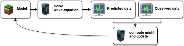
Full-waveform inversion (FWI) is non-linear data-fitting procedure that aims at obtaining detailed estimates of subsurface properties from seismic data, which can be the result of either passive or active seismic experiments. Given an initial guess of the subsurface parameters, (a model) the data are predicted by solving a wave-equation. The model is then updated in order to reduce the misfit between the observed and predicted data. This is repeated in an iterative fashion until the data-misfit is sufficiently small. A schematic overview is given below.

Mathematically, we can formulate this as an optimization problem for \(M\) experiments \[ \begin{equation} \min_{\mathbf{m}} \phi(\mathbf{m}) = \sum_{i=1}^M \rho(F_i(\mathbf{m}) - \mathbf{d}_{i} ), \label{misfit} \end{equation} \] where \(\mathbf{m}\) represents the physical model and \(\rho(\cdot)\) is a penalty function. Inside the penalty, \(\mathbf{d}_i = \mathbf{d}_1,\ldots,\mathbf{d}_M\) are the observed data and \(F_i = F_1,\ldots,F_M\) is the corresponding modelling operator for the \(i^\mathrm{th}\) experiment. The optimization problem is typically solved using iterative algorithms of the form \[ \begin{equation} \mathbf{m}_{k+1} = \mathbf{m}_{k} + \alpha_{k}\mathbf{s}_k, \label{steepest} \end{equation} \] where \(\mathbf{s}_k\) is called the search direction and \(\alpha_k\) is a steplength. The simplest instance is the steepest-descent algorithm, in which case the search direction is given by the negative gradient of the objective \(\mathbf{s}_k = -\nabla\phi(\mathbf{m}_k)\).

Algorithms

Scalable FWI with randomized trace estimation

Because reverse-time-migration (RTM) can be interpreted as a single FWI gradient, we can directly apply our imaging with random trace estimation to inversion and scale our algorithm to 3D on accelerators (GPUs) thanks to extremely low memeory imprint of this method. We show on Figure #3dtest the first gradient computed on the 3D overthrust model using 32 probing vectors (X50 memory reduction compared to standard adjoitn-state). This gradient was computed on Azure, using our cloud native extension of JUDI, JUDI4Cloud, and ran on Standard_NC6 instances consiting of a single K80 NVIDIA GPU withotu any need for streaming or offloading for the forward wavefield.

While we were able to compute this gradient given the scarce resources available, we are always looking for partenrship and collaboration to have access to the computational resources for a full at-scale 3D inversion experiement.

Dimensionality reduction and stochastic optimization

Evaluation of the misfit (Equation \(\ref{misfit}\)) and the computation of its gradient are very expensive operations, which involve \(2M\) solutions of the numerical partial differential equation (PDE-solves) for every iteration. Dimensionality reduction aims to dramatically reduce the total data volume by either random subsampling or random superposition. However, this introduces an error in the gradient when compared to the more complete search direction computed using all data. By using techniques from stochastic optimization, we can devise optimization methods that can deal with such errors. For more details see Leeuwen and Herrmann (2013a), Aravkin et al. (2012).

Modified Gauss–Newton

The Gauss-Newton method is one way to solve the FWI inverse problem. It is an efficient alternative to Newton’s method to solve non-linear least squares problems. Using the second-order Gauss–Newton method instead of the first-order steepest-descent method (Equation \(\ref{steepest}\)) may dramatically speed up convergence. However, each iteration is more expensive as it involves solving an overdetermined linear system to obtain the search direction \[ \begin{equation} \min_{\mathbf{s}} \sum_{i=1}^M ||\nabla F_i(\mathbf{m}_k)\mathbf{s} - \mathbf{r}_{i}||_2^2, \label{gaussnewton} \end{equation} \] where \(\mathbf{r}_i = \mathbf{d}_{i} - F_i(\mathbf{m}_{k})\). Again, we can use the techniques from dimensionality reduction and stochastic optimization to speed up these computations. Since this will turn the previously overdetermined system into an underdetermined one, regularization needs to be added. One successful approach is based on an \(\ell_1\) regularization in conjunction with a Curvelet transform \(C\): \[ \begin{equation} \min_{\mathbf{x}} \sum_{i=1}^M ||\nabla F_i(\mathbf{m}_k)C^*\mathbf{x} - \mathbf{r}_{i}||_2^2\quad\mathrm{s.t.}\quad ||\mathbf{x}||_1\leq \tau, \label{modgaussnewton} \end{equation} \] With this approach we are able to compute Gauss–Newton updates at roughly the cost of a full gradient calculation. For more details, see Li et al. (2012).

Robust FWI

Robust FWI aims to improve noise tolerance in waveform inversion procedures. Typically, one uses a least-squares penalty function to formulate the FWI misfit (i.e., \(\rho(\mathbf{r}) = ||\mathbf{r}||_2^2\); see Equation \(\ref{misfit}\)). However, when the data are contaminated with large outliers, this may lead to severe artifacts in the final result. In this case, robust penalties like the Huber or Student’s t may improve the result because they measure the model misfit according to a probability density function (PDF) that is appropriate to the data. For more details, see Aravkin et al. (2012).

Estimation of nuisance parameters

In the application of full waveform inversion methods, it may be necessary to estimate additional parameters that are not part of the previously-described model result (see introduction), such as the source-weights or noise-variances. The optimization problem can now be written as the joint optimization problem in Equation \(\eqref{jointnuisance}\) \[ \begin{equation} \min_{\mathbf{m},\theta} \phi(\mathbf{m},\theta), \label{jointnuisance} \end{equation} \] where \(\theta\) represents the additional parameters. In a many applications, the optimisation over \(\theta\) for a fixed \(\mathbf{m}\) can be done cheaply since it does not involve any additional forward simulations. This motivates us to replace the joint optimization problem by a reduced problem \[ \begin{equation} \min_{\mathbf{m}} \overline\phi(\mathbf{m}) = \phi(\mathbf{m},\overline\theta(\mathbf{m})), \label{reducedobjective} \end{equation} \] where \[ \begin{equation*} \overline\theta(\mathbf{m}) = \mathrm{argmin}_{\theta}\, \phi(\mathbf{m},\theta). \end{equation*} \] The crux is that the gradient of the reduced objective (Equation \(\ref{reducedobjective}\)) can be computed in a straightforward manner: \(\nabla\overline\phi(\mathbf{m}) = \nabla\phi(\mathbf{m},\overline\theta) \). Thus, the estimation of nuisance parameters can be easily included in an existing FWI workflow. For more details, see Aravkin and Leeuwen (2012).

Wavefield Reconstruction Inversion (WRI)

Wavefield Reconstruction Inversion is a new method developed by SLIM that is similar to FWI, but with some significant benefits (patent pending; see Leeuwen and Herrmann, 2014). WRI is designed to mitigate some of the problems related to missing low-frequency data and poor start models, which leads to the cycle-skip phenomenon. The method generates ‘wavefields’ (called data-augmented wavefield) which satisfy the observed data as well as the physics of wave propagation in a least-squares sense. Because this will cause the fields to fit the data to some extend, regardless of the startmodel, this method does not get stuck in a local minimum right after the start of the optimization process, but allows updating of the velocity model in the right direction. The software corresponding to this section can be found at here (imaging) and here(waveform inversion).

The general waveform inversion problem is described by PDE-constrained optimization problem (in discrete form): \[ \begin{equation} \min_{\bm,\bu} \frac{1}{2}\| P \bu- \bd\|^{2}_{2} \quad \text{s.t.} \quad A(\bm) \bu = \bq. \label{prob_state} \end{equation} \] where \(P\) is a linear projection operator onto the receiver locations, \(A\) is the discretized two-parameter Helmholtz matrix, \(\bu\) is the pressure wavefield, \(\bq\) is the source term and \(\bd\) is the measured data. We invert for \(\bm\), the slowness squared.

The most common way to solve this problem is to form a Lagrangian and apply the adjoint-state method to obtain gradients which can be used in gradient-descent type methods or quasi-Newton methods.

Leeuwen and Herrmann (2013b) and Leeuwen and Herrmann (2013c) recently proposed a different way for solving the model-recovery problem named Wavefield Reconstructing Inversion (WRI). This approach removes the constraint (Equation \(\ref{prob_state}\)) and adds the PDE to the objective as a quadratic penalty term: \[ \begin{equation} \min_{\bm,\bu} \phi_{\lambda}(\bm,\bu) = \frac{1}{2}\| P \bu - \bd\|^{2}_{2} + \frac{\lambda^2}{2}\|A(\bm)\bu -\bq\| ^{2}_{2}. \label{obj_full} \end{equation} \] Equation \(\eqref{obj_full}\) is a weighted sum of the data-misfit and the PDE-misfit, where the scalar \(\lambda\) determines the importance of each. This is now an unconstrained problem. We proceed by applying a variational projection as in Aravkin and Leeuwen (2012) to eliminate the field variable by solving \[ \begin{equation} \begin{split} \bar{\bu}= \arg\min_{\bu} \bigg\| \begin{pmatrix} \lambda A(\bm) \\ P \end{pmatrix} \bu-\begin{pmatrix} \lambda \bq \\ \bd \end{pmatrix} \bigg\|_2 \end{split} \label{DAW} \end{equation} \] to obtain the reduced form \[ \begin{equation} \min_{\bm} \bar{\phi}_{\lambda}(\bm) = \frac{1}{2}\| P \bar{\bu} - \bd\|^{2}_{2} + \frac{\lambda^2}{2}\|A(\bm)\bar{\bu} -\bq\| ^{2}_{2} . \label{objred} \end{equation} \] Using this formulation, we update the fields \(\bar{\bu}\) first, and then update the medium parameters. In other words, we first reconstruct the wavefield, given the PDE and observed data, then we use that field to update the model. At each iteration of an optimization algorithm, we solve the least-squares problem and find an update direction using an appropriate method (e.g., steepest descent, quasi-Newton or Gauss–Newton). The misfit and gradients can be accumulated as a running sum over frequencies and sources. Therefore, only one field has to be in memory at a time. No adjoint fields are required with this formulation.

Example 1

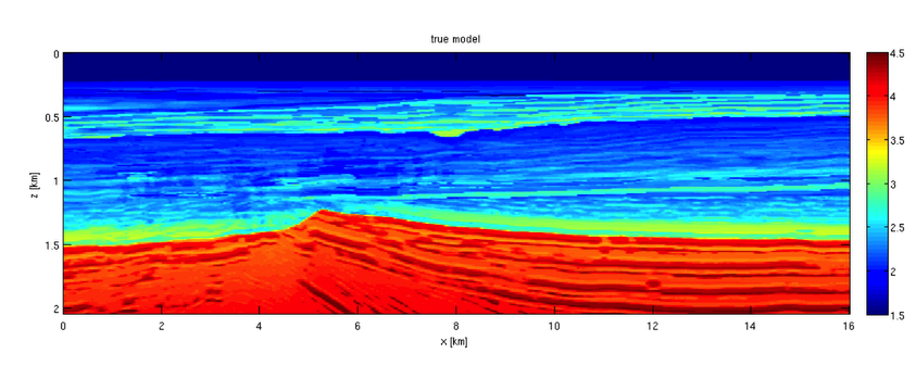
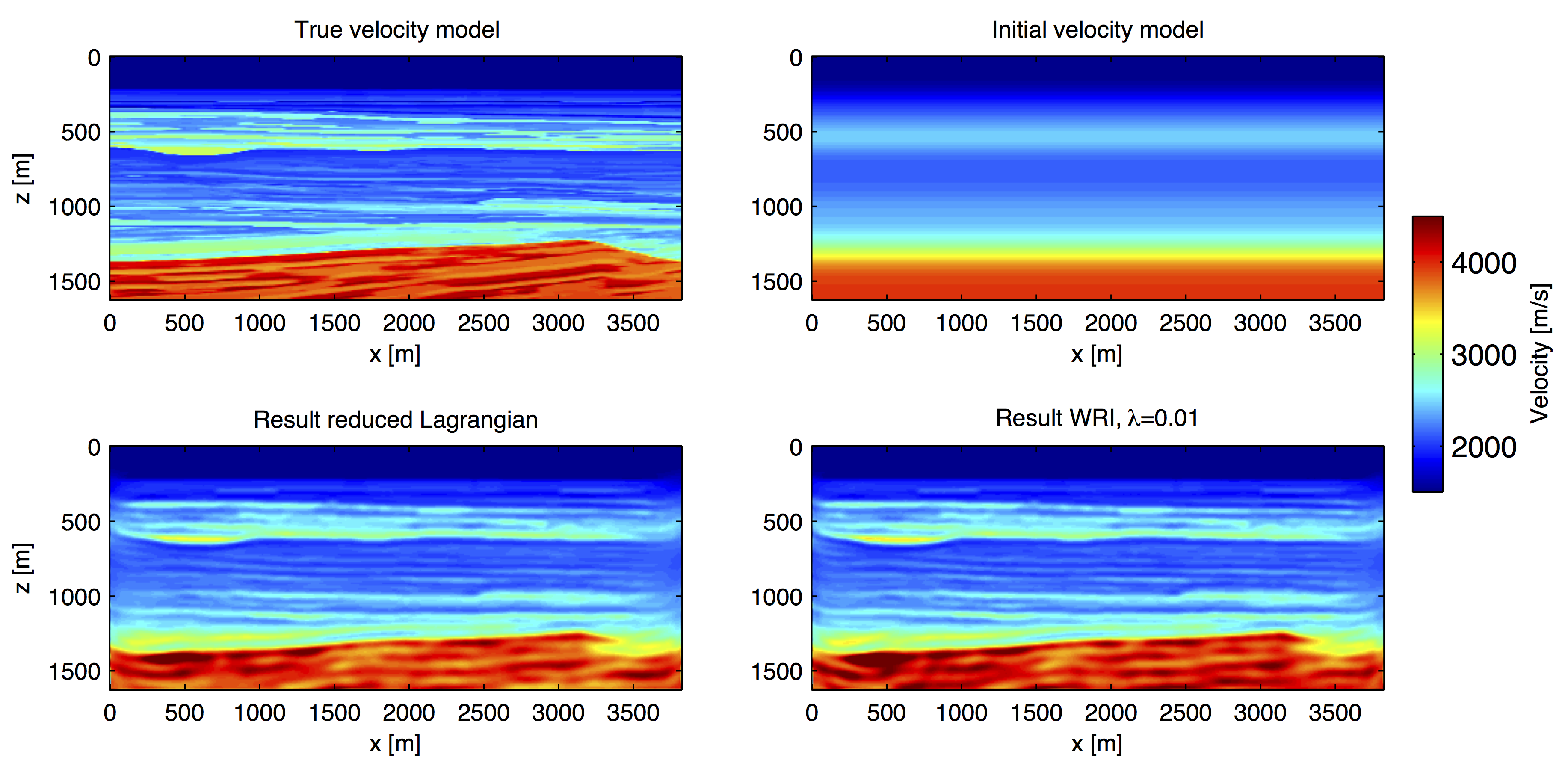
This example is from Peters et al. (2014). Figure 6 illustrates that both the reduced Lagrangian (conventional FWI; Equation \(\ref{prob_state}\)) and the WRI method (Equation \(\ref{objred}\)) give similar and good results when there is no noise in the data and an accurate starting model is used. Sources and receivers are near the surface and spread over the horizontal coordinate. A frequency continuation approach was used to invert the data in frequency batches as \(\{2,3\}, \{3,4\}, ...,\{19,20\}\) Hz.

Example 2

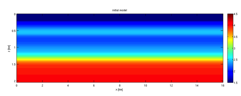
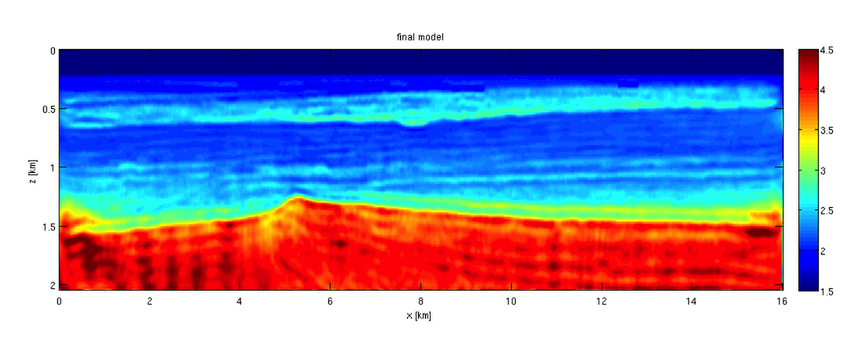
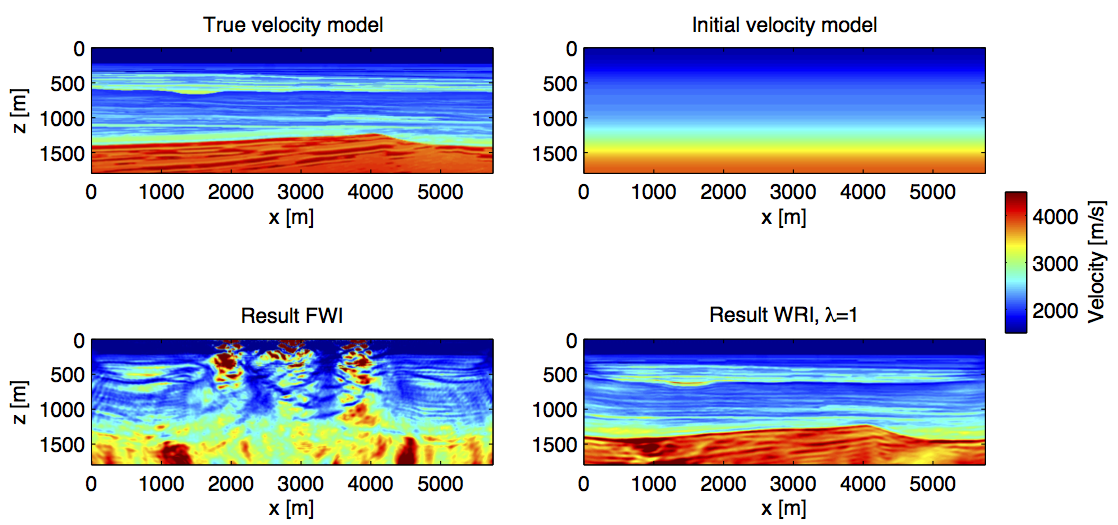
This example from Peters et al. (2014) shows the power of the WRI formulation of the waveform inversion problem. Here we start with an inaccurate initial model (Figure 7) and no low-frequency data. The frequency batches are \(\{5, 5.25, 5.5, 5.75, 6\}, \{6, 6.25, 6.5, 6.75, 7\}, \ldots, \{27, 27.25, 27.5, 27.75, 28\}, \{5, 5.25, 5.5, 5.75, 6\}, \{6, 6.25, 6.5, 6.75, 7\}, \ldots, \{27, 27.25, 27.5, 27.75, 28\}\) Hertz.

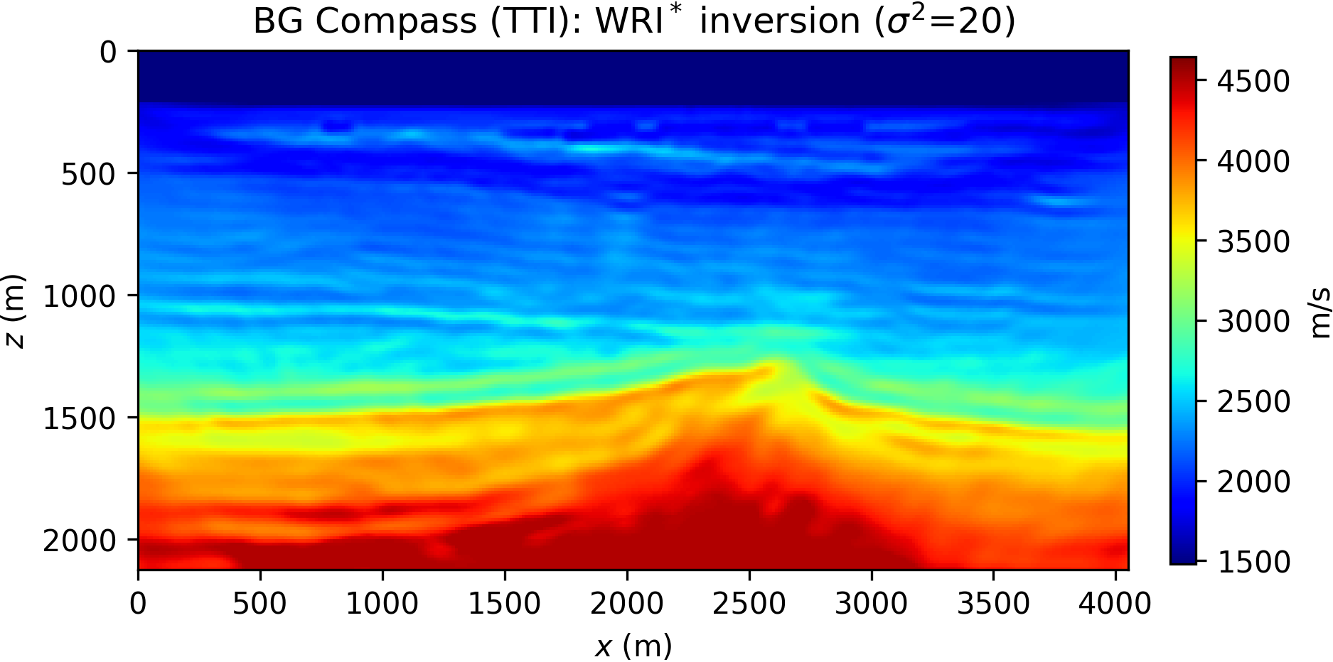
Time-domain WRI

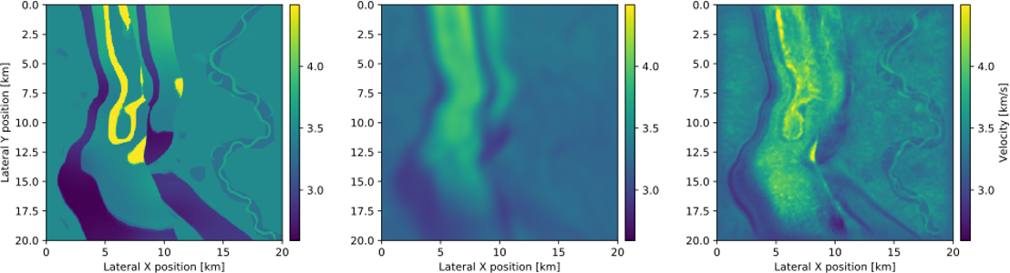
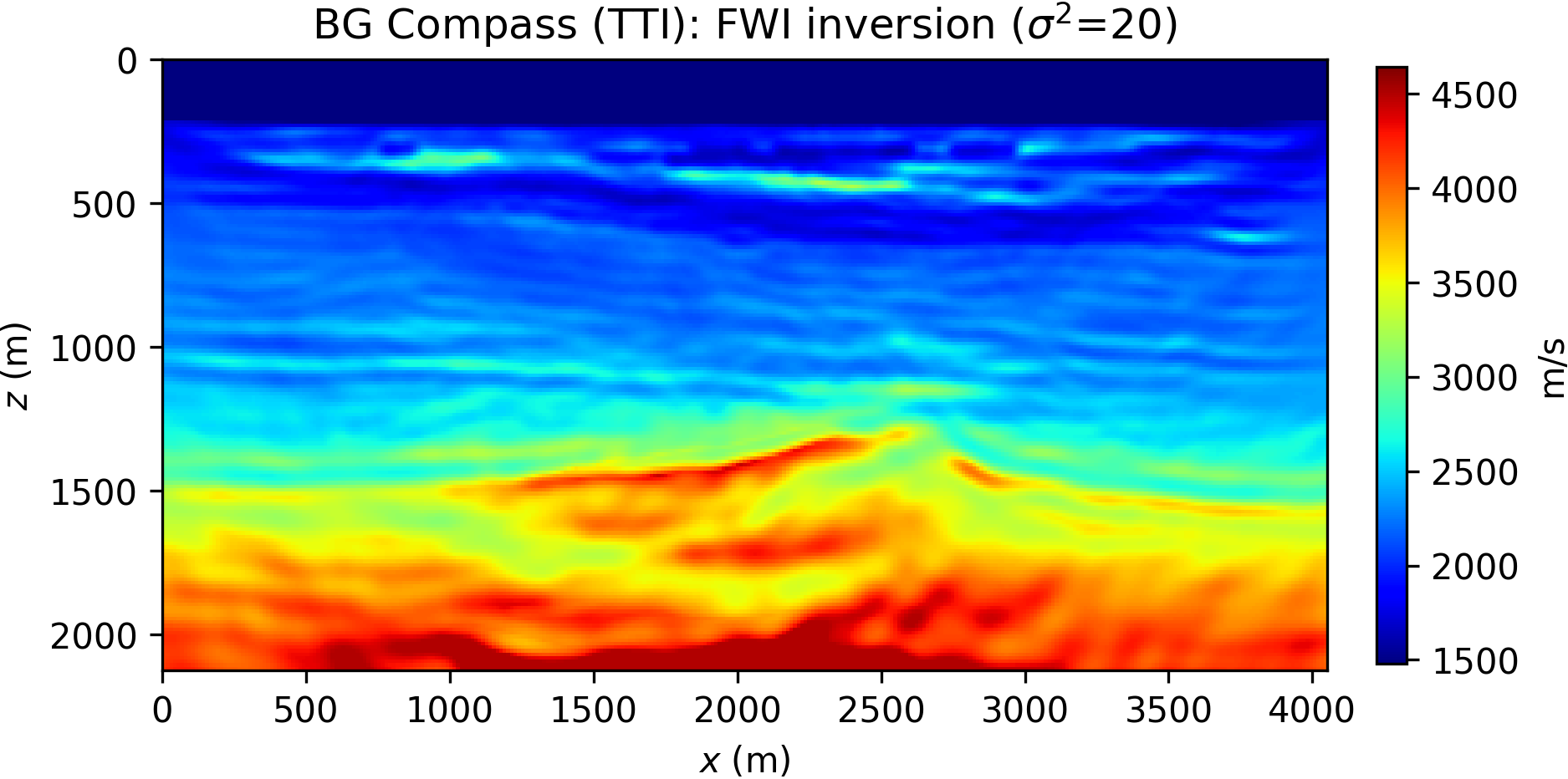
While solving the extended system in Equation \(\ref{DAW}\) is feasible in the frequency domain (by solving the augmented Helmholtz equation with direct matrix inversion), obtaining its solution in the time-domain is unrealistic because of the size of the matrices involved both in 2D and especially in 3D. Because of our strong focus on scalable solutions that can be directly applied to 3D field data, we introduce a time-domain formulation of WRI that suits time stepping propagators well (Wang and Herrmann, 2017; Rizzuti et al., 2020, 2021; Louboutin et al., 2020). This reformulation, while relying on few additional PDE solves, offers similar advantages in regard to cycle skipping than its frequency domain counterpart. The time-domain WRI formulation is defined as the minimization of the following reduced Lagrangian: \[ \begin{equation} \begin{split} & \max_{\by}\min_{\bmm}\LWRId(\bmm,\by),\\ & \LWRId(\bmm,\by)=-\dfrac{1}{2}\norm{\F^{\ast}\by}^2+\<\by,\br\>-\epsilon\norm{\by}, \end{split} \label{eq:TWRI} \end{equation} \] where \(\F\) is the standard time-domain forward modeling operator. Additionally, since its implementation is based on Devito and JUDI, we were able to easily extend existing acoustic isotropic results to TTI models, which are more representative of the true wave physics. In Figure 8, we show a selected example of inversion in a TTI medium. Additional examples and analysis can be found in our Time-domain WRI paper. These examples are fully reproducible and can be found at JUDI-WRI as part of our seismic inversion abstraction JUDI.

Intuition

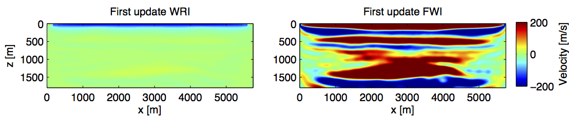
We can provide some visual intuition why the reduced Lagrangian method (conventional FWI) and WRI result in very different models. Figure 9 shows the first update at the first iteration for the first frequency batch for Example 2. It shows that the WRI method starts updating the area near the sources/receivers first. The reduced Lagrangian update is oscillating and updating everywhere, but not always in the correct direction. This leads to quick stagnation of the optimization algorithm; a local minimizer is found far away from the true model. This example is described in Peters et al. (2014).

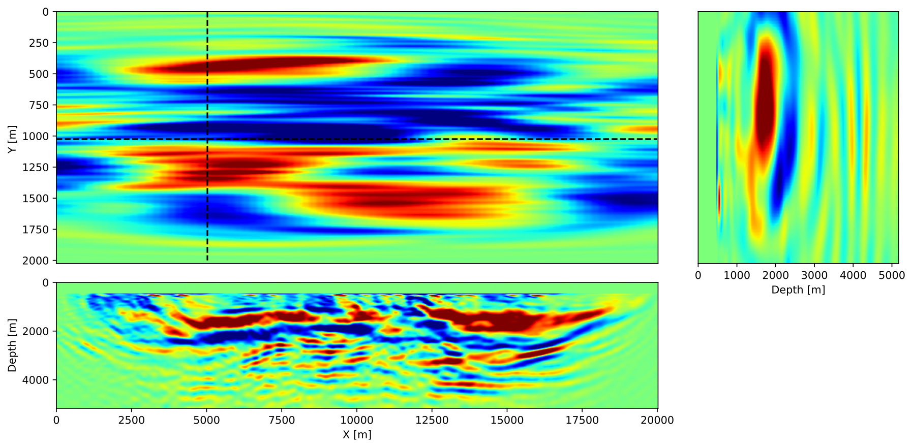
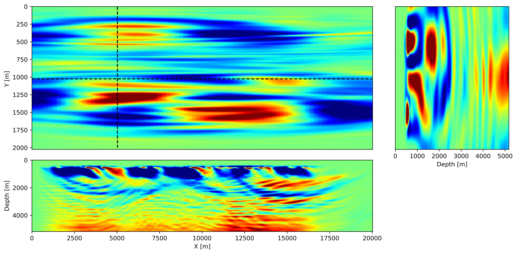
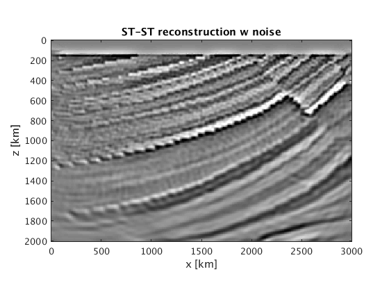
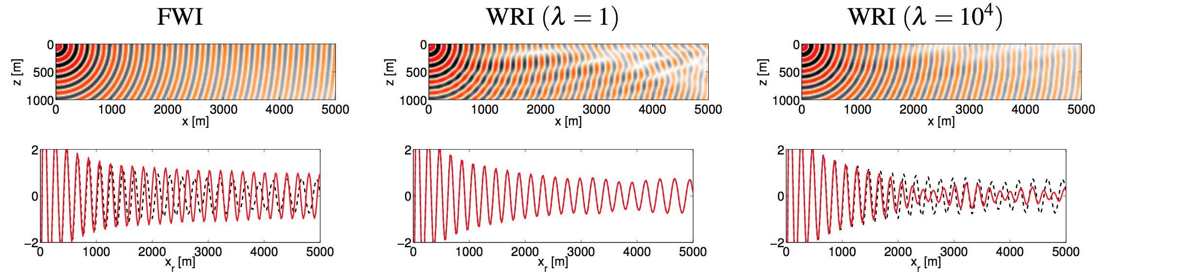
It is also useful to look at the wavefield computed by the Helmholtz equation using the current model estimate as is done in the reduced Lagrangian method and compare it to the wavefield estimate that is computed by the WRI method, using the current model estimate as well as the observed data; see Figure 10 for a toy example. This is explained in Leeuwen et al. (2014).

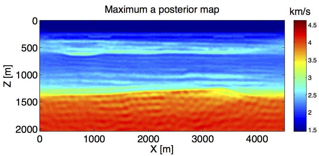
Uncertainty quantification for FWI

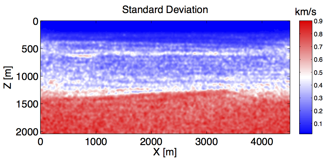
Uncertainty analysis is important for seismic interpretation. However, in the field of full waveform inversion, research associated to the uncertainty quantification is rare due to the huge computational cost of solving wave equations. In this work, we try to present a computational tractable method based on the Bayesian framework to analyze different statistical parameters of the FWI result. Suppose the observed data \(\mathbf{d}_{obs}\) is perturbed by additive Gaussian noise with zero mean and a covariance matrix \(\Gamma_{noise}\), and suppose the prior probability density of the model parameters is represented as Gaussian with \({\mathbf{m}_{prior}}\) as the mean and \(\Gamma_{prior}\) as the covariance matrix; then, the posterior probability density formula (pdf) of the model parameters is given explicitly by \[ \begin{equation*} \pi_{post}(\mathbf{m}) := \pi(\mathbf{m}|\mathbf{d}_{obs}) \propto \pi_{prior}(\mathbf{m})\pi(\mathbf{d}_{obs}|\mathbf{m}) \label{eq:Bay} \end{equation*} \] where the likelihood function \(\pi(\mathbf{d}_{obs}|\mathbf{m})\) is \[ \begin{equation*} \pi(\mathbf{d}_{obs}|\mathbf{m}) = \exp[{-||\mathbf{F}(\mathbf{m})-\mathbf{d}_{obs}||_{\Gamma^{-1}_{noise}}^{2}}] \end{equation*} \] and the prior probability function is \[ \begin{equation*} \pi_{prior}(\mathbf{m}) = \exp[{-||\mathbf{m}-\mathbf{m}_{prior}||^{2}_{\Gamma^{-1}_{prior}}}] \end{equation*} \] It is computationally intractable to use the posterior pdf to calculate the statistical parameters we want, due to the high dimension of the model size and the huge computational cost of the forward modeling. In order to make it computationally tractable, we present a stochastic quasi Newton Markov chain Monte Carlo (McMC) method to speed up the convergence and reduce the computational cost. Based on this technique, we can obtain the statistic parameters we want approximately. More detail to see Fang et al. (2014) and Zhilong Fang and Lee (2014).

Also check constrained FWI and time-lapse FWI.

References

Aravkin, A. Y., and Leeuwen, T. van, 2012, Estimating Nuisance Parameters in Inverse Problems: Inverse Problems, 28. doi:10.1088/0266-5611/28/11/115016
Aravkin, A. Y., Friedlander, M. P., Herrmann, F. J., and Leeuwen, T. van, 2012, Robust Inversion, Dimensionality Reduction, and Randomized Sampling: Mathematical Programming, 134, 101–125. doi:10.1007/s10107-012-0571-6
Fang, Z., Silva, C. D., and Herrmann, F. J., 2014, Fast Uncertainty Quantification for 2D Full-waveform Inversion with Randomized Source Subsampling: 76th eAGE. Retrieved from https://slim.gatech.edu/Publications/Public/Conferences/EAGE/2014/fang2014EAGEfuq/fang2014EAGEfuq.pdf
Leeuwen, T. van, and Herrmann, F. J., 2013a, Fast Waveform Inversion without Source-Encoding: Geophysical Prospecting, 61, 10–19. Retrieved from http://dx.doi.org/10.1111/j.1365-2478.2012.01096.x
Leeuwen, T. van, and Herrmann, F. J., 2013b, Mitigating local minima in full-waveform inversion by expanding the search space: Geophysical Journal International, 195, 661–667. doi:10.1093/gji/ggt258
Leeuwen, T. van, and Herrmann, F. J., 2013c, A penalty method for pDE-constrained optimization: UBC. Retrieved from https://slim.gatech.edu/Publications/Private/TechReport/2013/vanLeeuwen2013Penalty2/vanLeeuwen2013Penalty2.pdf
Leeuwen, T. van, and Herrmann, F. J., 2014, A penalty method for PDE-constrained optimization (CONFIDENTIAL): UBC; UBC. Retrieved from https://slim.gatech.edu/Publications/Public/Patents/2014/herrmann2014pmpde/vanLeeuwen2014pmpde_original.pdf
Leeuwen, T. van, Herrmann, F. J., and Peters, B., 2014, A new take on fWI: Wavefield reconstruction inversion: EAGE. UBC; UBC. Retrieved from https://slim.gatech.edu/Publications/Public/Conferences/EAGE/2014/leeuwen2014EAGEntf/leeuwen2014EAGEntf.pdf
Li, X., Aravkin, A. Y., Leeuwen, T. van, and Herrmann, F. J., 2012, Fast Randomized Full-waveform Inversion with Compressive Sensing: Geophysics, 77, A13–A17. doi:10.1190/geo2011-0410.1
Louboutin, M., Rizzuti, G., and Herrmann, F. J., 2020, Time-domain wavefield reconstruction inversion in a tTI medium: ArXiv Preprint ArXiv:2004.07355.
Peters, B., Herrmann, F. J., and Leeuwen, T. van, 2014, Wave-equation based inversion with the penalty method: Adjoint-state versus wavefield-reconstruction inversion: EAGE. UBC; UBC. Retrieved from https://slim.gatech.edu/Publications/Public/Conferences/EAGE/2014/peters2014EAGEweb/peters2014EAGEweb.pdf
Rizzuti, G., Louboutin, M., Wang, R., and Herrmann, F. J., 2020, Time-domain wavefield reconstruction inversion for large-scale seismics: In 82nd eAGE annual conference & exhibition (Vol. 2020, pp. 1–5). European Association of Geoscientists & Engineers.
Rizzuti, G., Louboutin, M., Wang, R., and Herrmann, F. J., 2021, A dual formulation of wavefield reconstruction inversion for large-scale seismic inversion: Geophysics, 86, 1ND–Z3. doi:10.1190/geo2020-0743.1
Wang, R., and Herrmann, F., 2017, A denoising formulation of full-waveform inversion: In SEG technical program expanded abstracts 2017 (pp. 1594–1598). Society of Exploration Geophysicists.
Witte, P. A., Louboutin, M., Kukreja, N., Luporini, F., Lange, M., Gorman, G. J., and Herrmann, F. J., 2019, A large-scale framework for symbolic implementations of seismic inversion algorithms in julia: Geophysics, 84, F57–F71. doi:10.1190/geo2018-0174.1
Zhilong Fang, F. J. H., and Lee, C. Y., 2014, A stochastic quasi-newton McMC method for uncertainty quantification of full-waveform inversion: UBC; UBC. Retrieved from https://slim.gatech.edu/Publications/Public/TechReport/2014/zfang2014SEGsqn/zfang2014SEGsqn.html