Optimization

Introduction

Structure-promoting optimization and Optimization with constraints have and continue to play a key role in the development of seismic wavefield recovery as part of Acquisition, Processing, Compressive Imaging, Full-waveform inversion. At SLIM, we have made considerable efforts towards the development of several scalable (convex) optimization techniques culminating in an extensive body of work including

• early work on Sparse recovery by Gilles Hennenfent, Ewout van den Berg, Michael P. Friedlander, and Felix J. Herrmann, “New insights into one-norm solvers from the Pareto curve”, Geophysics, vol. 73, pp. A23-A26, 2008
• wavefield reconstruction via Matrix completion by Aleksandr Y. Aravkin, Rajiv Kumar, Hassan Mansour, Ben Recht, and Felix J. Herrmann, “Fast methods for denoising matrix completion formulations, with applications to robust seismic data interpolation”, SIAM Journal on Scientific Computing, vol. 36, pp. S237-S266, 2014
• Imaging with stochastic linearized Bregman by Emmanouil Daskalakis, Felix J. Herrmann, and Rachel Kuske, “Accelerating Sparse Recovery by Reducing Chatter”, SIAM Journal on Imaging Sciences, vol. 13, pp. 1211–1239, 2020
• Full-waveform inversion with constraints by Ernie Esser, Lluís Guasch, Tristan van Leeuwen, Aleksandr Y. Aravkin, and Felix J. Herrmann, “Total-variation regularization strategies in full-waveform inversion”, SIAM Journal on Imaging Sciences, vol. 11, pp. 376-406, 2018
• Projection on the intersection of multiple constraint sets by Bas Peters, Brendan R. Smithyman, and Felix J. Herrmann, “Projection methods and applications for seismic nonlinear inverse problems with multiple constraints”, Geophysics, vol. 84, pp. R251-R269, 2018.

Below, we provide highlights.

Structure-promoting optimization

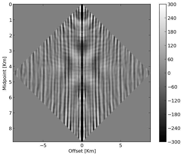
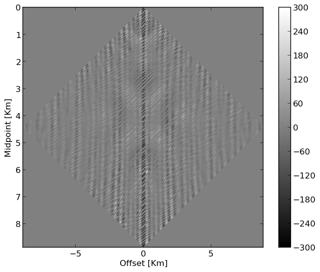
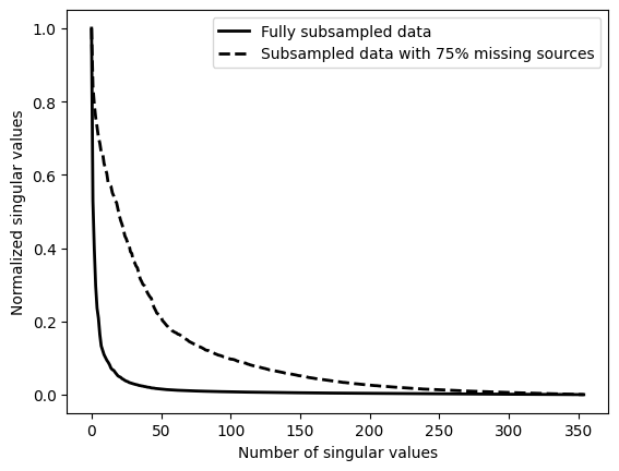
During the early stages of oil and gas exploration and during monitoring of e.g. Geological Carbon Storage, Acquisition of seismic data is essential but expensive. Compressive Sensing (Candès et al., 2006) can be used to improve efficiency of this step. Throughout Compressive Sensing, seismic data is collected randomly along spatial coordinates to improve acquisition productivity and reduce costs (see e.g. randomized marine acquisition). While random sampling increases acquisition productivity (Mosher et al., 2014, A. Aravkin et al. (2014)), it shifts the burden from data Acquisition to data Processing (Chiu, 2019) because densely periodically sampled data are often required by subsequent data Processing steps such as multiple removal and Imaging. Among the different wavefield reconstruction approaches, low-rank matrix factorization (Kumar et al., 2015) represents a relatively simple and scalable approach, which utilizes low-rank structure exhibited by densely regularly sampled data organized in matrix form in the midpoint-offset domain by monochromatic frequency slices. As shown by Kumar (2017), fully sampled seismic lines are low rank—i.e, they can well be approximated while randomly subsampled seismic lines are not low rank. Juxtapose the decay of singular in Figure 1 between fully sampled and randomly sample 2D data from the Gulf. Wavefield reconstruction exploits this property, which extends to permuted monochromatic 3D seismic data organized in non-canonical form by lumping source/receiver coordinates together rather than combining the two source and receiver coordinates together (Da Silva and Herrmann, 2015).

Below, we use (weighted) Matrix completion techniques that exploit this low-rank structure to perform wavefield reconstruction.

Matrix completion

(Software overview available here)

Julia code for (weighted) Matrix completion is available here

When completing a matrix from missing entries using approaches from convex optimization, see (A. Y. Aravkin et al., 2013), the following problem \[ \begin{equation} \underset{\mathbf{X}}{\operatorname{minimize}} \|\mathbf X\|_* \quad \text{subject to} \quad \|\mathcal{A}(\mathbf X) - b\|_2 \le \sigma \label{bpdn} \end{equation} \] is solved. While minimizing the nuclear norm \(\|\mathbf X\|_*\) promotes low-rank structure in the final solution—i.e., there are no guarantees that intermediate solutions are low rank, it is difficult to solve (\(\ref{bpdn}\)) directly as it is a constrained problem with a non-smooth objective. Instead, we solve problems where the nuclear norm (\(\|\cdot\|_\ast\) equals sum of singular values) constraint and data-misfit objective are interchanged \[ \begin{equation} \underset{\mathbf{X}}{\operatorname{minimize}}\quad \|\mathcal{A}(\mathbf X) - b\|_2^2 \quad \text{subject to} \quad \|\mathbf X\|_* \le \tau. \label{lasso} \end{equation} \] We solve these problems for a sequence of algorithmically chosen relaxed parameters \(\tau\), eventually resulting in a solution of Problem \(\ref{bpdn}\). These problems can be solved in a straightforward manner using a projected-gradient method involving the following steps: \[ \begin{equation*} \begin{aligned} \mathbf X_{k+1} &= P_{\tau}(\mathbf X_{k} - \alpha_{k} g_k ) \\ \\ P_{\tau}(\mathbf Y) &= \operatorname{argmin}_{\mathbf{Z}} \{ \|\mathbf Z - \mathbf Y\|_F \quad \text{subject to} \quad\|\mathbf Z\|_* \le \tau \} \end{aligned} \end{equation*} \] where \(g_k\) is the gradient of the objective.

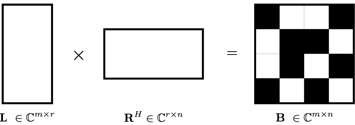
While elegant, the iterations of Problem \(\ref{lasso}\) rely on storage of the matrix \(\mathbf X\) and computation of its singular values, which unfortunately does not scale to 3D seismic volumes that have hundreds of thousands or even millions of rows and columns. In that case, computing the projection \(P_{\tau}(\mathbf Y)\), which involves computing the SVD of the matrix \(\mathbf Y\), becomes cost-prohibitive. To address this issue, we rely on the following approximation for the nuclear norm of \(\mathbf X\): \[ \begin{equation*} \|\mathbf X\|_* = \underset{\mathbf{L,R}}{\operatorname{minimize}}\quad \dfrac{1}{2} (\|\mathbf L\|_F^2 + \|\mathbf R\|_F^2), \quad \text{subject to} \quad \mathbf X = \mathbf {LR}^T \end{equation*} \] for matrices \(\mathbf L,\mathbf R\) of rank \(k\). If we replace \(\mathbf X\) in (\(\ref{lasso}\)) by \(\mathbf {LR}^T\), we can instead compute approximate projections on to the ball \[ \begin{equation} \{ (\mathbf L,\mathbf R) : \text{subject to} \; 1/2 (\|\mathbf L\|_F^2 + \|\mathbf R\|_F^2) \le \tau \}. \label{lrball} \end{equation} \] These projections involves computing the Frobenius norm of \(\mathbf L\) and \(\mathbf R\) and scaling both variables by a constant, which is considerably cheaper than computing the SVD of the original matrix \(\mathbf X\). By using this \(\mathbf {L,R}-\)factorization approach, we solve large scale matrix completion problems for completing seismic data from missing sources/receivers.

Weighted matrix completion

(More details information can be found in this SEG2019 abstract and SEG2020 abstract)

While SLIM utilized techniques from Matrix completion successfully for low to midrange frequencies, performance degrades at high frequencies due to the failure of low-rank factorization to accurately approximate monochromatic frequency slices (Zhang et al., 2019). Slider 1 is an illustration of reconstructing field data collected from Gulf of Suez with \(75\%\) missing sources using the conventional (non-weighted) matrix completion. Despite the fact that we successfully reconstructed the subsampled data, the slider 2, shows that the reconstruction lost high-frequency information.

Employing the fact that matrix factorizations at neighboring frequencies are likely to live in nearby subspaces, we perform weighted wavefield reconstruction by solving the following nuclear-norm minimization problem (A. Aravkin et al., 2014, Eftekhari et al. (2018), Zhang et al. (2019) and Zhang et al. (2020)): \[ \begin{equation} \underset{\mathbf{X}}{\operatorname{minimize}}\quad \|\mathbf{QXW}\|_* \quad \text{subject to} \quad \|\mathcal{A}(\mathbf X) - \mathbf{b}\|_2 \le \tau, \label{eqWlrmf} \end{equation} \] where the weighting matrices \(\mathbf Q\) and \(\mathbf W\) are projections given by \[ \begin{equation} {\mathbf Q} = {w}_{1}{\mathbf U}{\mathbf U}^H + {\mathbf U}^\perp {\mathbf U}^{{\perp}{H}} \label{eqprojl} \end{equation} \] and \[ \begin{equation} {\mathbf W} = {w}_{2}{\mathbf V}{\mathbf V}^H + {\mathbf V}^\perp {\mathbf V}^{{\perp}{H}}. \label{eqprojr} \end{equation} \] The matrices \(\mathbf U\) and \(\mathbf V\) contain the column and row subspaces derived from low-rank factorizations of adjacent frequency slices. The scalars \(w_1 \in (0,1]\) and \(w_2 \in (0,1]\) quantify the similarity between prior information and the current to-be-recovered data. Small values for these scalars indicate a greater degree of confidence in the prior information.

To prevent computationally expensive singular value decompositions (SVDs) part of the nuclear norm computations, we factorize Problem \(\ref{eqWlrmf}\) as follows (Zhang et al., 2019), \[ \begin{equation*} \begin{split} \underset{\mathbf{L}, \mathbf{R}, }{\operatorname{minimize}}\quad \frac{1}{2} {\left\| \begin{bmatrix} \mathbf {QL} \\ \mathbf{WR} \end{bmatrix} \right\|}_F^2 \quad \text{subject to} \quad \|\mathcal{A}(\mathbf{LR}^{H}) - \mathbf{b}\|_{2} \leq \tau, \end{split} \end{equation*} \] where matrices \(\mathbf{L}\) and \(\mathbf{R}\) have rank \(k\). By relocating the weighting matrices from the constraint to the data-misfit, Zhang et al. (2020) proposed a computationally efficient scheme capable of reconstructing high-frequency data.

Example

We apply the presented Weighted matrix completion technique on the same observed 2D field data. Slider 2 demonstrates the advantage of our proposed weighted method in comparison to conventional matrix completion.

To make weighted Matrix completion applicability to 3D seismic acquisition, we also developed a parallel implementation where the computations are decoupled on a row-by-row and column-by-column basis (see Figure 2) (Recht and Ré, 2013, Lopez et al. (2015))

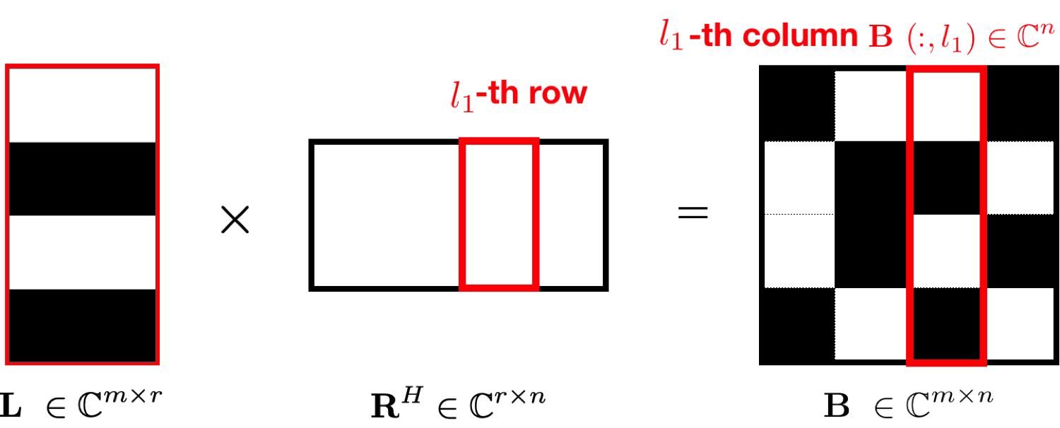
More details of this parallelization can be found in this manuscript.

Tensor completion

(Software overview available here)

We can also exploit the tensor structure of seismic data for interpolating frequency slices with missing sources or receivers.

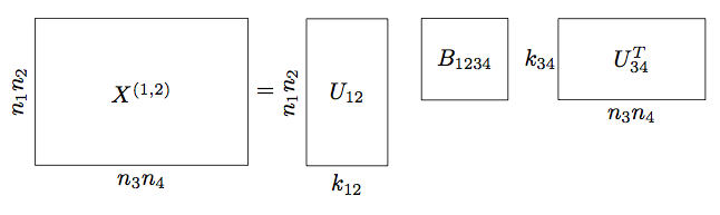
An efficient format for representing high dimensional tensors is the so-called Hierarchical Tucker (HT) format. As depicted in Figure 3, we first reshape the \(4D\) tensor \(\mathbf X\) in to a matrix by placing its first and second dimensions along the rows and the third and fourth dimensions along the columns, denoted \(\mathbf X^{(1,2)}\). We then perform an ‘SVD-like’ decomposition on \(\mathbf X^{(1,2)}\), resulting in the matrices \(\mathbf U_{12}\), \(\mathbf U_{34}\), and \(\mathbf B_{1234}\). The insight of the Hierarchical Tucker format is that the matrix \(\mathbf U_{12}\) contains the first and second dimensions along the rows, so when we reshape this matrix back in to a \(3-\)dimensional tensor, we can further ‘split apart’ dimension \(1\) from dimension \(2\) in this ‘SVD-like’ fashion.

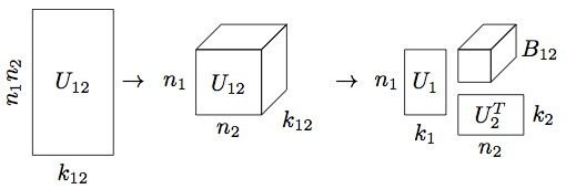
In the example above, the intermediate matrices \(\mathbf U_{12}, \mathbf U_{34}\) do not need to be stored: the small parameter matrices \(\mathbf U_i\) and small \(3-\) transfer tensors \(\mathbf B_t\) specify the tensor \(\mathbf{X}\) completely. The number of parameters needed to specify this class of tensors is bounded by \[ \begin{equation*} d N K + (d - 2) K^3 + K^2 \end{equation*} \] where \(d\) is the number of dimensions, \(N = \max_{i=1,\dots,d} n_i\) is the maximum individual dimension, and \(K\) is the maximum internal rank parameter. When \(K \ll N\) and \(d \ge 4\), this quantity is much less than \(N^d\) needed to store the full array, thus we avoid the curse of dimensionality.

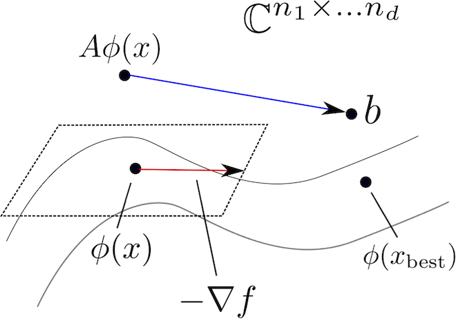
If we collect the HT parameters in a single vector \(x = (\mathbf U_t, \mathbf B_t)\) and we write \(\phi(x)\) for the fully expanded tensor, then the tensor completion problem we’re interested in solving is \[ \begin{equation*} \underset{x}{\operatorname{minimize}} \quad \dfrac{1}{2}\|\mathcal{A} \phi(x) - b\|_2^2. \end{equation*} \] The HT format exhibits the structure of a Riemannian manifold, which is a multidimensional generalization of smooth surfaces in \(\mathbb{R}^3\).

Results

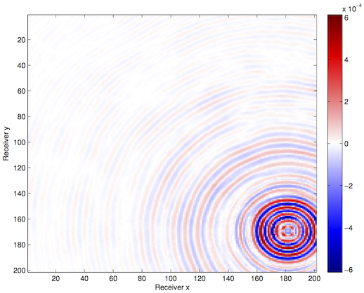
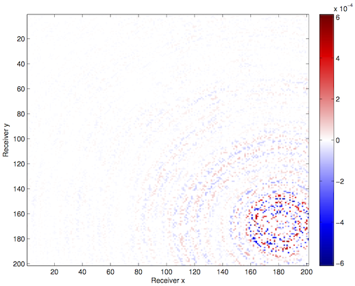
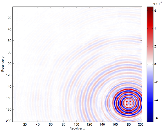
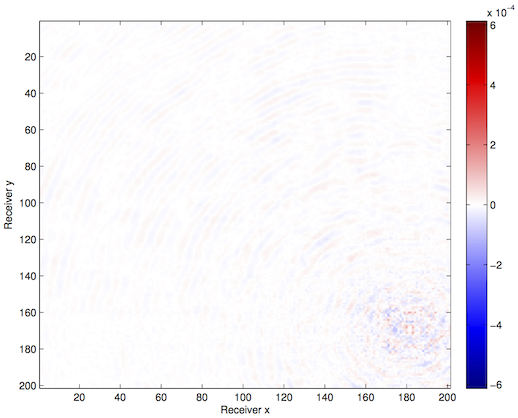
We apply these techniques to a synthetic frequency slice provided to us by BG Group, with 68 x 68 sources and 201 x 201 receivers. We randomly remove 75% of the receiver pairs from the volume and interpolate using our HT technique{–s–}.

Optimization with constraints

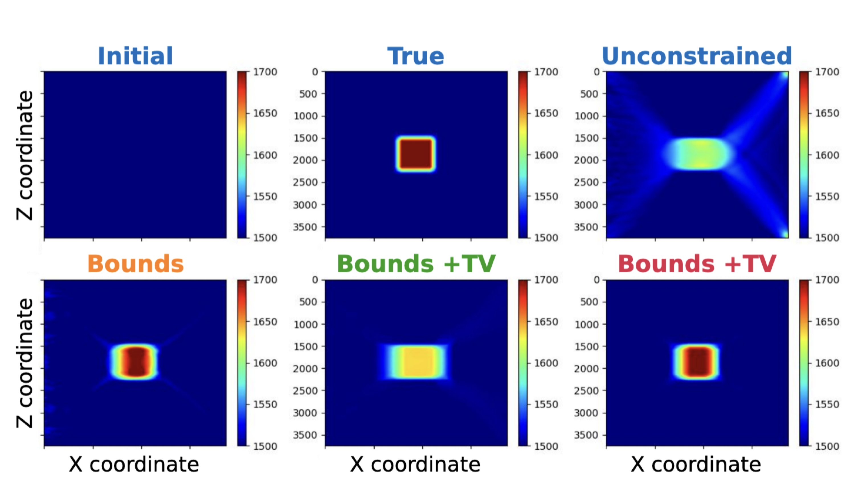
The use of techniques optimization do not limit themselves to Sparse recovery and Matrix completion but also include important results on the regularization of non-convex optimization problems such as Full-waveform inversion that are hampered by parasitic local minima. Our postdoc, the late Ernie Esser made, in collaboration with S-Cube, an important contribution by constraining Wavefield Reconstruction Inversion, a special type of Full-waveform inversion, with box, TV-norm, and hinge-loss constraints (Esser et al., 2018). See Figure 6.

By constraining the inversion, Ernie was able to avert local minima that hampered the application of Full-waveform inversion to salt. Motivated, by this early success we developed at SLIM a framework how to include prior information via multiple constraints into deterministic inversion problems (Peters and Herrmann, 2017; Peters et al., 2018). Given an arbitrary but finite number of constraint sets (\(p\)), a constrained optimization problem can be formulated as follows: \[ \begin{equation} \underset{\bm}{\operatorname{minimize}} \:\: f(\bm) \:\: \text{subject to} \:\: \bm \in \bigcap_{i=1}^p \mathcal{C}_i \label{prob-constr} \end{equation} \] where \(f(\bm): \mathbb{R}^N \rightarrow \mathbb{R}\) is the data-misfit objective that is minimized with respect to a vector with discrete parameters, e.g. the discretized medium parameters represented by the vector \(\bm \in \mathbb{R}^N\). Prior knowledge on this model vector resides in the indexed constraint sets \(\mathcal{C}_i, i=1 \cdots p\), each of which captures a known aspect of the Earth’s subsurface. These constraints may include bounds on permissible parameter values, desired smoothness or complexity, or limits on the number of layers in sedimentary environments and many others.

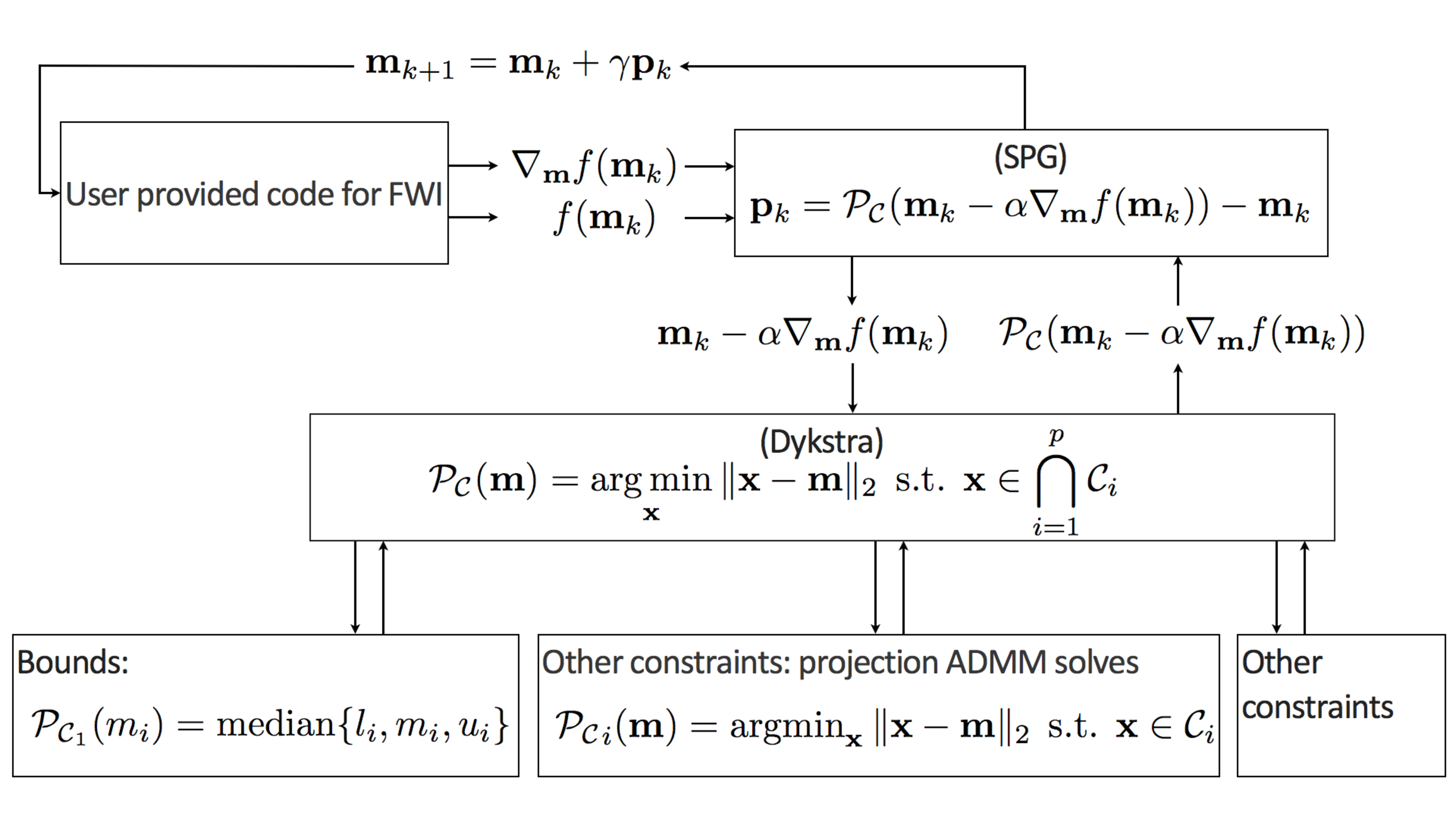
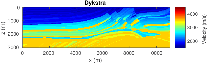
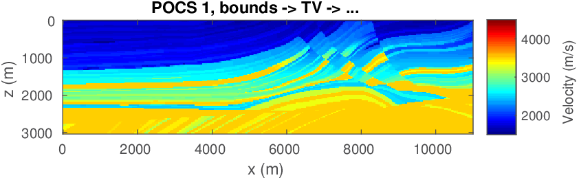
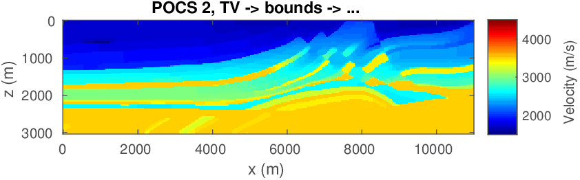
Compared to penalty formulations where prior information is included in the form of penalties, constrained formulations have the advantage that the model iterates during the optimization remain within the constraint set, which is important when inverting for parameters that need to remain physical. Since we are dealing with multiple constraint sets, we define the projection on the intersection of multiple sets as \[ \begin{equation} \mathcal{P_{C}}({\bm})=\operatorname*{arg\,min}_{\bx} \| \bx-\bm \|^2_2 \quad \text{s.t.} \quad \bx \in \bigcap_{i=1}^p \mathcal{C}_i. \label{def-proj} \end{equation} \] This projection of \(\bm\) onto the intersection of the sets, \(\bigcap_{i=1}^p \mathcal{C}_i\), corresponds to finding an unique vector \(\bx\) in the intersection of all sets, which is closest to \(\bm\) in an Euclidean sense. To find this vector, we initially used Dykstra’s alternating projection algorithm as outlined in Figure 7. We made this choice because this algorithm is relatively easy to implement (we only need projections on each set individually). An important advantage of this approach is that it avoids ambiguities of the method of projection onto convex sets (POCS), which may converge to different points, depending onto which set we project onto first. See Figure 8.

To meet the challenges to scale to 3D, we developed the Projection Adaptive Relaxed Simultaneous Method of Multipliers (PARSDMM) (Peters and Herrmann, 2019). This implementation is made available as open-source Julia package SetIntersectionProjection.jl on our GitHub site with this Documentation and Tutorial for parallel implementation.

Solvers

To take full advantage of our optimization framework, we implemented solvers specifically targeting constrained optimization in SlimOptim.jl. By computing update directions consistent with both the gradient of the objective function and the set of constraints (Schmidt et al., 2009), these algorithms take advantage of the mathematical structure of the constrained-optimization problem. Among the different approaches, we implemented the first-order spectral-projected gradient (SPG) method, its second-order counterpart of based on conjugate gradients, and projected Quasi-Newton (PQN), the constrained counterpart of L-BFGS. To facilitate interoperability with existing tools to compute gradients of the data-misfit objective (e.g. those provided by JUDI.jl) and to enforce projections onto intersections of multiple constraint sets (e.g. those provided by SetIntersectionProjection.jl), SlimOptim.jl’s interface closely resemble that of Optim.jl one of the most used optimization package in Julia. This allows users access to our solver within their existing inversion framework by simply swapping in our solvers (SlimOptim.jl) and constraints (SetIntersectionProjection.jl).

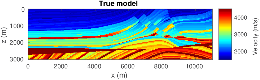
Two example notebooks are available. For given Constrained FWI examples, these demonstrate the advantage of using properly designed constraints in combination with these optimization.

References

Aravkin, A. Y., Kumar, R., Mansour, H., Recht, B., and Herrmann, F. J., 2013, An SVD-free Pareto curve approach to rank minimization: No. TR-EOAS-2013-2. UBC. Retrieved from https://slim.gatech.edu/Publications/Public/TechReport/2013/kumar2013ICMLlr/kumar2013ICMLlr.pdf
Aravkin, A., Kumar, R., Mansour, H., Recht, B., and Herrmann, F. J., 2014, Fast methods for denoising matrix completion formulations, with applications to robust seismic data interpolation: SIAM Journal on Scientific Computing, 36, S237–S266.
Candès, E. J., Romberg, J., and Tao, T., 2006, Robust uncertainty principles: Exact signal reconstruction from highly incomplete frequency information: IEEE Transactions on Information Theory, 52, 489–509.
Chiu, S. K., 2019, 3D attenuation of aliased ground roll on randomly undersampled data: In SEG international exposition and annual meeting. OnePetro.
Da Silva, C., and Herrmann, F. J., 2015, Optimization on the hierarchical tucker manifold – applications to tensor completion: Linear Algebra and Its Applications, 481, 131–173. doi:https://doi.org/10.1016/j.laa.2015.04.015
Eftekhari, A., Yang, D., and Wakin, M. B., 2018, Weighted matrix completion and recovery with prior subspace information: IEEE Transactions on Information Theory, 64, 4044–4071.
Esser, E., Guasch, L., Leeuwen, T. van, Aravkin, A. Y., and Herrmann, F. J., 2018, Total-variation regularization strategies in full-waveform inversion: SIAM Journal on Imaging Sciences, 11, 376–406. doi:10.1137/17M111328X
Kumar, R., 2017, Enabling large-scale seismic data acquisition, processing and waveform-inversion via rank-minimization: PhD thesis,. University of British Columbia.
Kumar, R., Da Silva, C., Akalin, O., Aravkin, A. Y., Mansour, H., Recht, B., and Herrmann, F. J., 2015, Efficient matrix completion for seismic data reconstruction: Geophysics, 80, V97–V114.
Lopez, O., Kumar, R., and Herrmann, F. J., 2015, Rank minimization via alternating optimization-seismic data interpolation: In 77th eAGE conference and exhibition 2015 (Vol. 2015, pp. 1–5). European Association of Geoscientists & Engineers.
Mosher, C., Li, C., Morley, L., Ji, Y., Janiszewski, F., Olson, R., and Brewer, J., 2014, Increasing the efficiency of seismic data acquisition via compressive sensing: The Leading Edge, 33, 386–391.
Peters, B., and Herrmann, F. J., 2017, Constraints versus penalties for edge-preserving full-waveform inversion: The Leading Edge, 36, 94–100. doi:10.1190/tle36010094.1
Peters, B., and Herrmann, F. J., 2019, Algorithms and software for projections onto intersections of convex and non-convex sets with applications to inverse problems: ArXiv E-Prints. Retrieved from http://arxiv.org/abs/1902.09699
Peters, B., Smithyman, B. R., and Herrmann, F. J., 2018, Projection methods and applications for seismic nonlinear inverse problems with multiple constraints: Geophysics, 84, R251–R269. doi:10.1190/geo2018-0192.1
Recht, B., and Ré, C., 2013, Parallel stochastic gradient algorithms for large-scale matrix completion: Mathematical Programming Computation, 5, 201–226.
Schmidt, M., Berg, E., Friedlander, M., and Murphy, K., 2009, Optimizing costly functions with simple constraints: A limited-memory projected quasi-newton algorithm: In D. van Dyk & M. Welling (Eds.), Proceedings of the twelth international conference on artificial intelligence and statistics (Vol. 5, pp. 456–463). PMLR. Retrieved from https://proceedings.mlr.press/v5/schmidt09a.html
Silva, C. D., and Herrmann, F. J., 2015, Optimization on the Hierarchical Tucker manifold - applications to tensor completion: Linear Algebra and Its Applications, 481, 131–173. doi:10.1016/j.laa.2015.04.015
Zhang, Y., Sharan, S., and Herrmann, F. J., 2019, High-frequency wavefield recovery with weighted matrix factorizations: In SEG technical program expanded abstracts 2019 (pp. 3959–3963). Society of Exploration Geophysicists.
Zhang, Y., Sharan, S., Lopez, O., and Herrmann, F. J., 2020, Wavefield recovery with limited-subspace weighted matrix factorizations: In SEG international exposition and annual meeting. OnePetro.