Medical imaging
Introduction
At SLIM, we have accumulated expertise in high-fidelity subsurface imaging for decades. Recently, we have transferred this expertise into the field of medical imaging. Although the models of interest in these two fields exist on vastly different scales (tens of meters vs single micrometers) the fundamental problems in their simulations and inverse problems have huge overlap. As a central tool, Devito allows us to model wave equation PDEs at scale, even for large 3D simulations as shown in Figure 1. Using the user friendly interface of JUDI, we quickly prototype and then develop realistic simulations in photoacoustic imaging, limited-view computed tomography (CT) and magnetic resonance imaging (MRI). At SLIM we appreciate the importance of uncertainty quantification in medical imaging and this integrates with the focus we have on risk aware solutions to inverse problems. Here we present a few of our examples of our ongoing research in medical imaging.
Photoacoustic simulations
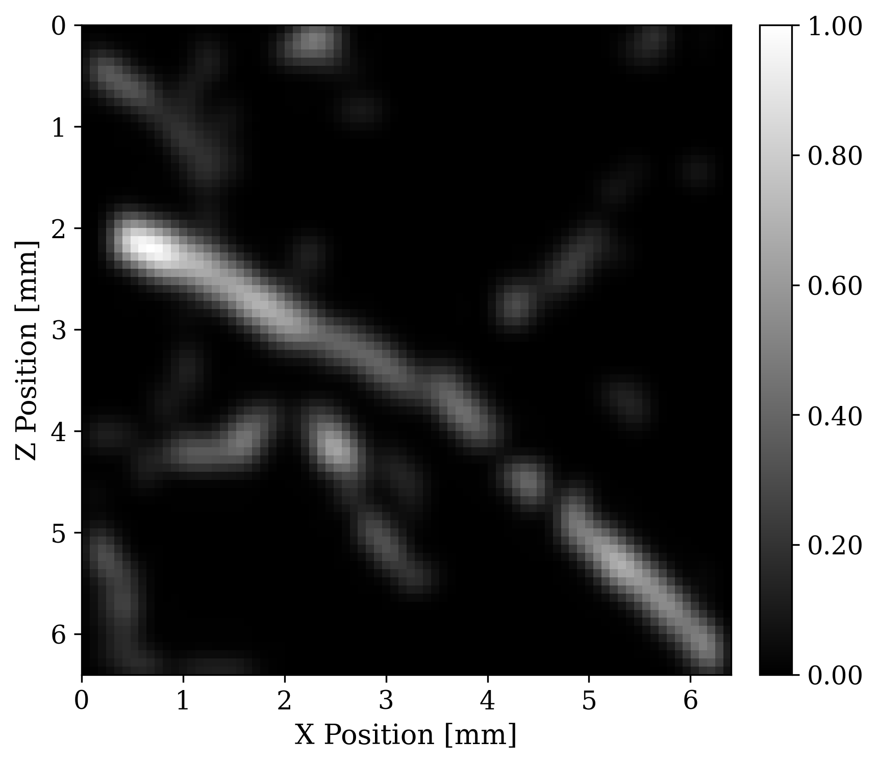
The principles of photoacoustic (PA) imaging are based on the interplay between light and acoustics. A light source is applied to the imaging area and light-sensitive molecules called chromophores produce acoustic wavefields that can be measured at a sensing array outside the tissue. In humans, this interaction is dominated by chromophores of iron present in blood cells. Thus for human tissue, blood vessels provide the highest contrast in photoacoustic images. Blood vessel images provide important information on a variety of clinical applications such as tumor growth monitoring, measuring oxygenation levels and tracking drug absorption. Creating a photoacoustic image is an inverse problem that aims to recover the initial source inside tissue from sensed acoustic wavefields outside the tissue.
The forward problem of photoacoustic imaging is the solution of a hyperbolic wave partial differential equation (PDE). This PDE solves the initial value problem of propagating a acoustic wavefield \(p\) given an initial source spatially distributed along \(p_0\): \[ \begin{equation} \begin{aligned} \left\{ \begin{array}{rcl} c^{-2}\partial_{tt}p-\Delta p & = &0\\ \partial_t p|_{t=0} & = & 0\\ p|_{t=0} & = & p_0. \end{array} \right. \end{aligned} \label{eq:1} \end{equation} \] The wave equation is linear in the source \(p_{0}\) so we will represent the forward process by operator \(A\). This operator will represents the forward propagation of an initial acoustic source \(p_0\) that we will name \(x\) for consistency with linear problem notation. During forward propagation, acoustic waves are sensed at an array of receivers. Due to geometric restrictions, this array typically is a limited view of the complete outgoing waveform. In a typical setup for human tissue imaging, receivers are placed on top of model (Z=0). By sensing the wavefield at the receiver array and degrading the observed data with noise \(\varepsilon\) we arrive to our familiar linear forward problem: \(y = Ax + \varepsilon\).
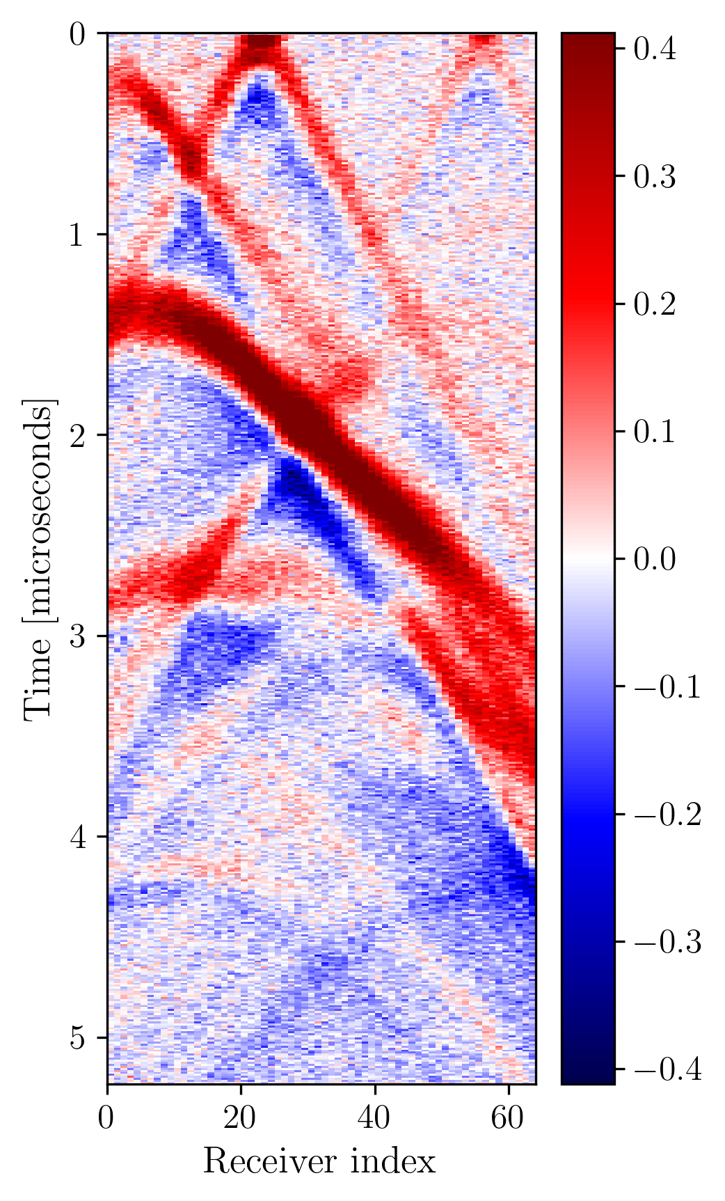
To illustrate this modality, we run 2D forward simulations and record the outgoing wavefield at a linear array of receivers positioned at the top of the model. The sensing array has \(64\) receivers. The recording is for \(N_{t}=519\) time steps and with \(dt = 10\) nanoseconds sampling. To simulate the forward and adjoint waveforms we used Devito, and JUDI, a Julia framework that wraps Devito propagators in user-friendly linear algebra notation . Each forward and adjoint simulation takes \(0.03\) seconds on a 4 core Intel Skylake CPU. To simulate realistic receivers, we degrade the sensed data with additive Gaussian noise \(\mathcal{N}(0,\sigma_{\varepsilon}^2 I)\) where the value of \(\sigma_{\varepsilon}\) results in an SNR of around 10dB for our data. Figure 2 shows an example of observed data.
Photoacoustic adjoint
When doing inverse problems it is important to have access to the adjoint of the forward operator. The adjoint allows us to calculate gradients for downstream least-squares based reconstrutions. This operator will also allow us to intuitively understand difficulties of photoacoustic imaging due to limited view of the receivers geometry. We derived the adjoint of the photoacoustic operator for the 2nd-order wave equation. Implementing the PDE of the forward and its adjoint is straight forward in the JUDI/DEVITO framework.
Memory efficient data-driven 3D Photoacoustic imaging
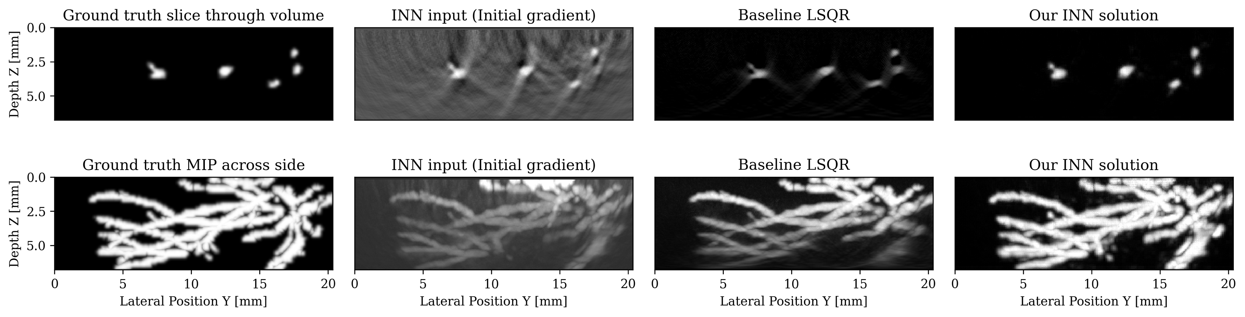
We tackle here the realistic case of limited-view, noisy and subsampled data, which makes the inverse problem ill-posed. Multiple solutions \(x\) can explain the data \(y\), therefore, this problem is typically solved in a variational framework where prior knowledge of the solution is incorporated by solving the minimization of the combination of an \(\ell_2\) data misfit \(L\) and a regularization term \(p_{\mathrm{prior}}(x)\). The success of this formulation hinges on users carefully selecting hyperparameters by hand such as the optimization step length and the prior itself, typically a multipurpose generic prior such as TV norm. On the other hand, recent machine learning work argues that we can learn the optimal step length and even a prior. We pursue this avenue and select loop-unrolled networks since this learned method also leverages the known physics of the problem encoded in the model \(A\).
Loop unrolled networks emulate gradient descent where the \(i^{\text{th}}\) update is reformulated as the output of a learned network \(\Lambda_{\theta_{i}}\): \[ \begin{equation} x_{i+1}, s_{i+1} = \Lambda_{\theta_{i}}(x_{i},s_{i}, \nabla_{x}L(A,x_{i},y)) \label{eq:loopunrolled} \end{equation} \] where \(s\) is a memory variable and \(\nabla_{x}L\) is the gradient w.r.t the data misfit on observed data \(y\). In our photoacoustic case, \(A\) is a linear operator (discrete wave equation) and \(L\) is \(\ell_2\) norm data misfit so the desired gradient is \(\nabla_{x}L(A,x_{i},y) = A^{\top}(Ax_{i}-y)\). Thus, each gradient will require two PDE solves: one forward and one adjoint. These wave propagations embed the known physical model into the learned approach. show that this method gives promising results on 3D photoacoustic but note that they are limited to training shallow networks due to memory constraints. To improve on this method, we propose using an INN that is an invertible version of loop-unrolled networks.
Our invertible neural network (INN) is based on the work of , where they propose an invertible loop-unrolled method called invertible Recurrent Inference Machine (i-RIM). While typical loop-unrolled approaches have linear memory growth in depth , i-RIM has constant memory usage due to its invertible layers. A network constructed with invertible layers does not need to save intermediate activations thus trading computation cost required to recompute activations for extremely frugal memory usage. We adapt i-RIM to Julia and make our code available alongside other invertible neural networks at .
Wave-based ultrasound imaging
We have developed projects in wave equation based ultrasound imaging to detect tissue anomalies close to the theoretical limit of given frequencies.
Extended source imaging
In extended source imaging, we are using an solved source to perform imaging of a subsurface medium. The non-linear term that we are solving for is the velocity model \(m\) and the linear term is the spatial location of the source \(u\). Here we assume that we know the wave source signature. In the case of our experiments this is a ricker wavelet. This leads to the formulation given seismic data d
\[
\begin{equation}
\min_{\mathbf{m},\,\mathbf{u}}{f}(\mathbf{m},\,\mathbf{u})=\frac{1}{\sigma^2}\sum_{i=1}^{n_s}\|\mathbf{d}_i-{F}[\mathbf{m}]\ast_t\mathbf{{q}}^e[\mathbf{u}_i]\|_2^2+\lambda R_x(\mathbf{u}_i)
\label{eq:opto}
\end{equation}
\]
From this expression we can start to formulate a variable projection method to solve for the optimal \(m\) and \(u\):
\[
\begin{equation}
\min_{\mathbf{m}} \bar{f}(\mathbf{m})=f(\mathbf{m},\,\bar{\mathbf{u}}(\mathbf{m}))\quad\text{where}\quad\mathbf{\bar{u}}=\argmin_{\mathbf{u}}f(\mathbf{m},\,\mathbf{u})
\label{eq:reduced-opto}
\end{equation}
\]
The gradient to this equation is given by the adjoint of the Jacobian wrt to the model given the source.
\[
\begin{equation}
\mathbf{g}=\nabla \bar{f}(\mathbf{m})=\frac{1}{\sigma^2}\sum_{i=1}^{n_s}\nabla\mathbf{F}^{\top}\left(\mathbf{d}_i-F[\mathbf{m}]\ast_t\mathbf{q}[\mathbf{\bar{u}}_i]\right)
\label{eq:gradient-opto}
\end{equation}
\]
Now that we have a formulation, for a gradient on the velocity model we will propose a novel imaging method for the photoacoustic case.
Breast calcifications
Contrary to seismic imaging, the field of medical imaging comprises of a wide range of different imaging modalities where different external stimuli are used to create an image with induced ultrasonic waves. Photoacoustic imaging is a good example of such an approach where laser light induces ultrasonic contrast sources.However, we can take this imaging modality a step further by using the methodology of extended source. Contrary to conventional photoacoustic imaging, we use these contrasts as “active” sources insonifying the specimen as a whole.
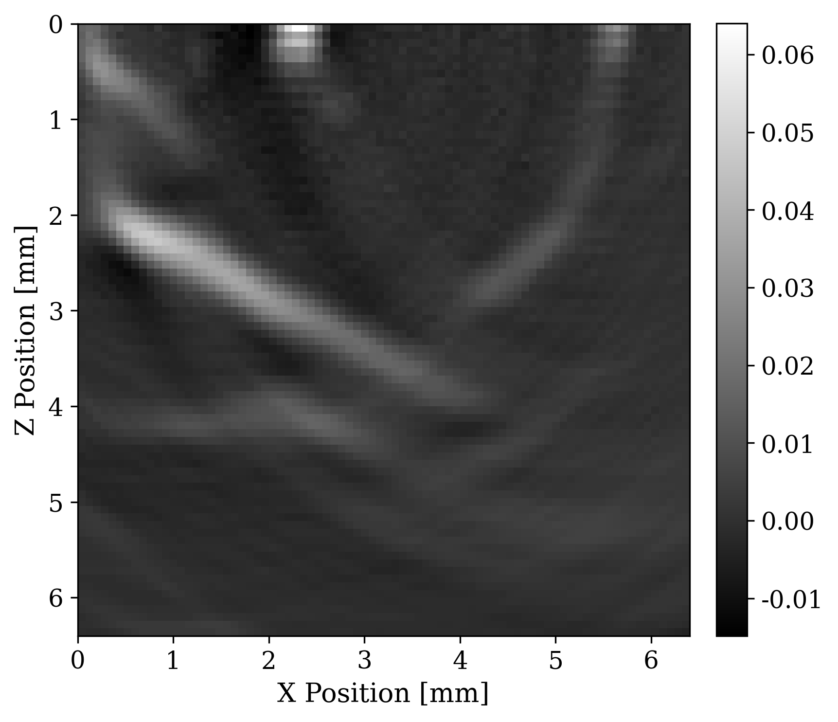
For this purpose, let us consider a 2D example of breast imaging where we are interested in finding microcalcifications (calcium oxalate) that could be indicative of breast cancer. In order to simulate a biologically correct breast, we took a horizontal slide of a 3d breast phantom from [lou2017generation] and added the following speed of sound values for each tissue.
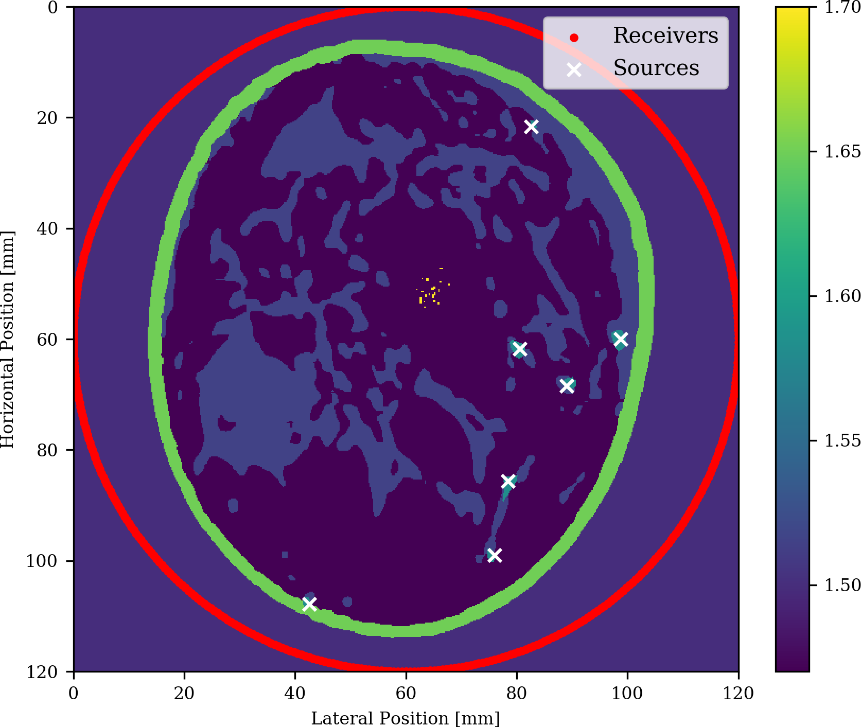
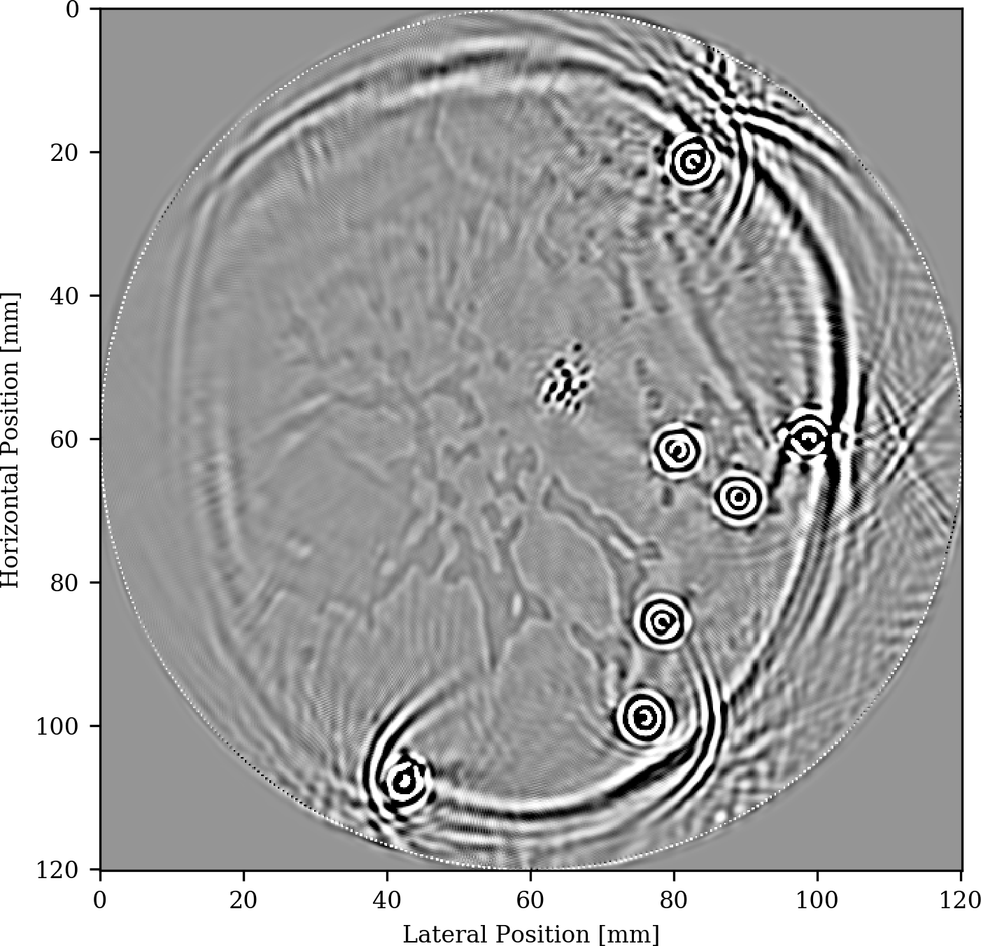
The setup for our experiment is depicted in Figure 5 and includes 7 different opto-induced sources placed in blood vessels and denoted by the white crosses and densely sampled receivers placed in a circular fashion around the breast. As we can see, we obtain a clear image not only of the microcalcifications but also of the fat and fibroglandular tissue
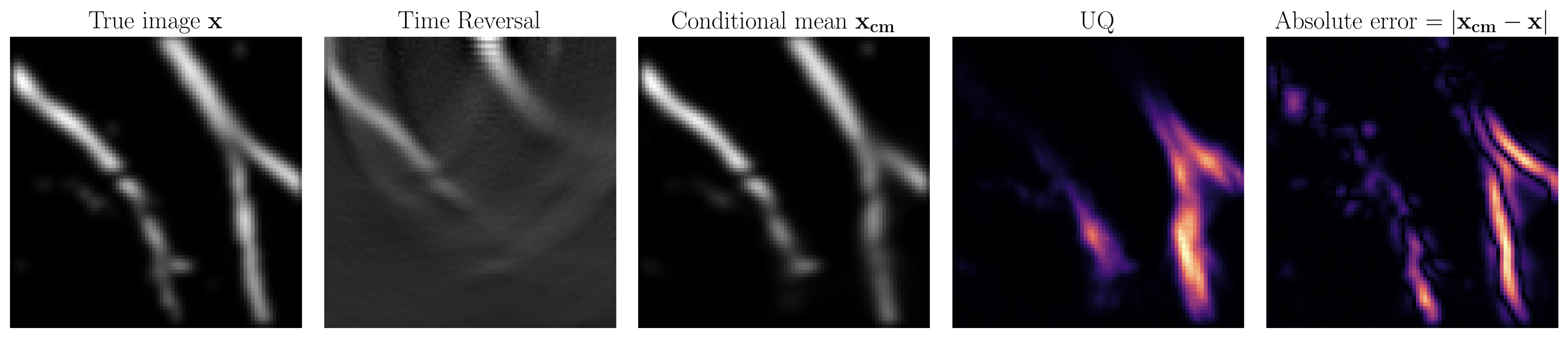
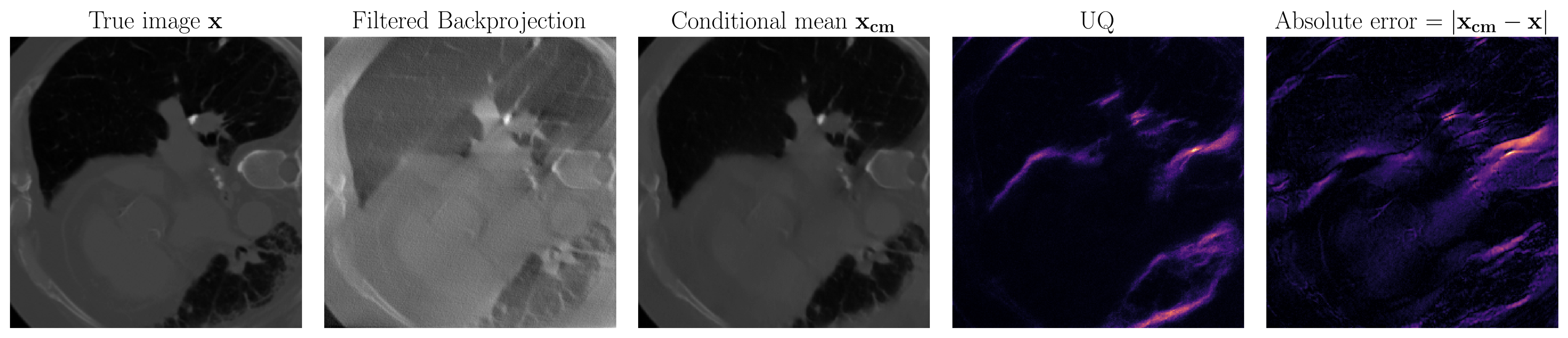
Medical imaging uncertainty quantification
At SLIM, we have advanced techniques in conventional UQ such as with the Laplace approximation. Recently, we have explored data-driven techniques for two reasons. Firstly, we can not assume a gaussian prior on our models of interest. Data-driven methods learn the prior from data so do away with this unrealistic gaussian assumption. Secondly, the medical imaging field is particularly interested in real-time results so we would like our final method to be fast. This is accomplished in data-driven techniques by trading an intensive training phase for fast inference that only requires evaluation of neural networks. To satisfy these requirements, the techniques we use are based on conditional normalizing flows.