
Time-lapse seismic
Introduction
With the gradual shift from exploration to production and even monitoring of Geological Carbon Storage, we at SLIM have worked extensively on how to improve time-lapse data Acquisition, Processing, and Imaging while increasing acquisition productivity, lowering cost without replicating the surveys. This work inspired by earlier work on Distributed Compressive Sensing has resulted in an extensive body of work that has appeared in the literature and when proven valid in the field can lead to major cost savings. Our contributions include
Felix Oghenekohwo, Haneet Wason, Ernie Esser, and Felix J. Herrmann, “Low-cost time-lapse seismic with distributed compressive sensing––Part 1: exploiting common information among the vintages”, Geophysics, vol. 82, pp. P1-P13, 2017;
Haneet Wason, Felix Oghenekohwo, and Felix J. Herrmann, “Low-cost time-lapse seismic with distributed compressive sensing—Part 2: impact on repeatability”, Geophysics, vol. 82, pp. P15-P30, 2017;
Felix Oghenekohwo and Felix J. Herrmann, “Highly repeatable time-lapse seismic with distributed Compressive Sensing—mitigating effects of calibration errors”, The Leading Edge, vol. 36, pp. 688-694, 2017;
Felix J. Herrmann’s 2019 SEG Distinguished Lecture “Sometimes it pays to be cheap — Compressive time-lapse seismic data acquisition”.
These contributions form the basis of recent work to address the challenges of low-cost Monitoring of Geological Carbon Storage.
The main question we ask ourselves concerning randomized source acquisition is “Is it necessary to replicate time-lapse surveys to attain high degrees of repeatability (low NRMS values)?”. To answer this question, we consider the following three scenarios for static randomized-source marine acquisition:
On-the-grid acquisition where overlap between the baseline and monitor survey implies exact replication of the surveys
Calibrated off-the-grid acquisition where the baseline and monitoring acquisition geometries for the sources are not replicated but where the post-plot source positions are known accurately
Non-calibrated off-the-grid acquisition where the post-plot source positions are not known accurately
We discuss these three different scenarios based on a novel Processing and Imaging inversion methodology developed at SLIM, which is designed to explore information that is common between the baseline and monitor surveys.
Randomized 4-D acquisition and recovery methods
Ideally, 4-D acquisition design requires surveys to be highly repeatable (Lumley and Behrens, 1998; Landrø, 1999) so that differences due to changes in the acquisition do not manifest themselves as time-lapse changes in the subsurface. Within the current paradigm for time-lapse seismic acquisition, high degrees of repeatability are sought after by replicating the surveys— e.g. source/receivers positions are chosen to match as closely as possible spatially between surveys. Unfortunately, this can be a challenge especially in marine streamer acquisition where the streamer locations are often influenced by ocean currents. This type of operational challenges also may have an effect on the source locations. For that reason, there has been a shift from dynamic to static acquisitions where the receivers are either fixed, as in Permanent Reservoir Monitoring (PRM) / Ocean Bottom Cable (OBC) systems or in Ocean Bottom Node (OBN) surveys (Johnston, 2013; Eggenberger et al., 2014), where fair amount of control can be placed on the receivers. However, in all these cases, there can still be some degree of uncertainty in source/receiver locations. So, we ask the question — is it really necessary to replicate the surveys to get a high degree of repeatability for surveys collected with Compressive Sensing?
To answer this question, we follow the randomized acquisition scheme described in randomized-source marine acquisition to select random source locations for baseline and monitor surveys. Next, we investigate two following recovery strategies.
Independent recovery strategy
In this approach to randomized 4-D acquisition, where the sources can be off-the-grid, we solve sparsity-promoting programs for the baseline and monitor surveys independently by using the fact that the surveys are sparse in the curvelet domain (F. J. Herrmann and Hennenfent, 2008). Mathematically, this can be formulated as (Oghenekohwo et al., 2017; Wason et al., 2017) \[ \begin{equation*} \begin{split} \nonumber \tilde{\vector{x}}_1 = \argmin_{\vector{x}_1}\|\vector{x}_1\|_1 \quad \textrm{subject to} \quad \vector{y}_1 = \vector{A}_1\vector{x}_1,\\ \nonumber \tilde{\vector{x}}_2 = \argmin_{\vector{x}_2}\|\vector{x}_2\|_1 \quad \textrm{subject to} \quad \vector{y}_2 = \vector{A}_2\vector{x}_2, \end{split} \end{equation*} \] where \(\vector{y}_1\) and \(\vector{y}_2\) are the observed randomly subsampled baseline and monitor data, respectively; \(\vector{A}_1\) and \(\vector{A}_2\) are the measurement matrices formed from the sampling operator and the sparsifying transform (curvelet transform). During these sparse inversions, the sources are brought to a periodic grid via regularization, are interpolated, and source separated, so that overlapping simultaneous shots are demultiplexed.
Joint recovery method
In this approach, we adapt Baron et al. (2005) and solve a sparsity-promoting program, which designed to explicitly exploit the information shared between the baseline and monitor surveys. While distinct source locations are missing for each survey, our approach recovers the common component observed by the baseline and monitor surveys, innovations with respect to the common component for the individual vintages. 4-D differences are computed by subtracting the innovations of each survey. We write \(\vector{x}_1 = {\vector{z}_0} + \vector{z}_1\ \text{and}\ \vector{x}_2= {\vector{z}_0} + \vector{z}_2\), where \({\vector{z}_0}\) denotes the common component and \(\vector{z}_1,\vector{z}_2\) denote the innovations with respect to this common component.
Mathematically, we can formulate this novel approach as a joint optimization problem (Oghenekohwo et al., 2017): \[ \begin{equation*} \tilde{\vector{z}} = \argmin_{\vector{z}}\|\vector{z}\|_1 \quad \text{subject to} \quad \vector{y} = \vector{A}\vector{z}, \nonumber \end{equation*} \] where \(\vector{A} = \begin{bmatrix} {\vector{A}_1} & \vector{A}_{1} & \vector{0} \\ {\vector{A}_{2}} & \vector{0} & \vector{A}_{2} \end{bmatrix}\), \(\vector{z} = \begin{bmatrix} \vector{z}_0 \\ \vector{z}_1 \\ \vector{z}_2 \end{bmatrix}\), and \(\vector{y} = \begin{bmatrix} \vector{y}_1 \\ \vector{y}_2 \\ \end{bmatrix}\).
After solving for the common and innovation components collected in vector \(\vector{z}\), the recovery for baseline and monitor surveys can be computed by summing the common and innovation components. The time-lapse change between baseline and monitor surveys can be computed via subtraction of innovation components, as \(\vector{z}_2-\vector{z}_1\).
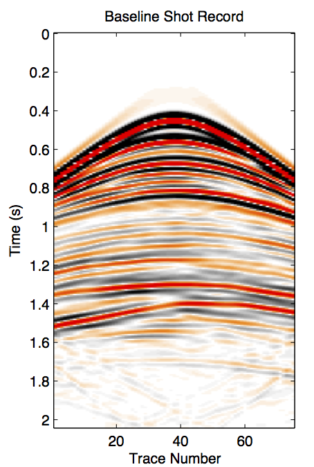
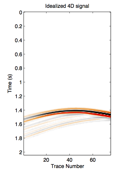
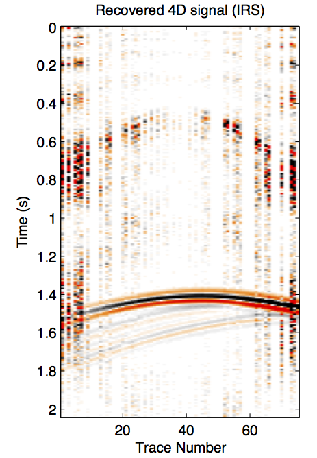
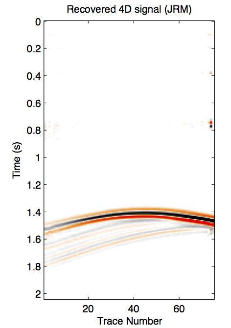
Figure 1 shows a synthetic experiment to compare the recovery results from the independent and joint recovery methods. The idealized time-lapse change between fully sampled baseline and monitor surveys is shown in Figure 1b. When the source locations are not replicated for the two surveys, the results from independent recovery and joint recovery are shown in Figure 1c and 1d. We can see strong artifacts when the shot records are independently recovered, but see a quite clean time-lapse recovered from joint recovery method.
Different static scenarios
To better understand the performance of Processing time-lapse data with the joint recovery model, we briefly discuss the three different scenarios mentioned in the Introduction.
On-the-grid acquisition
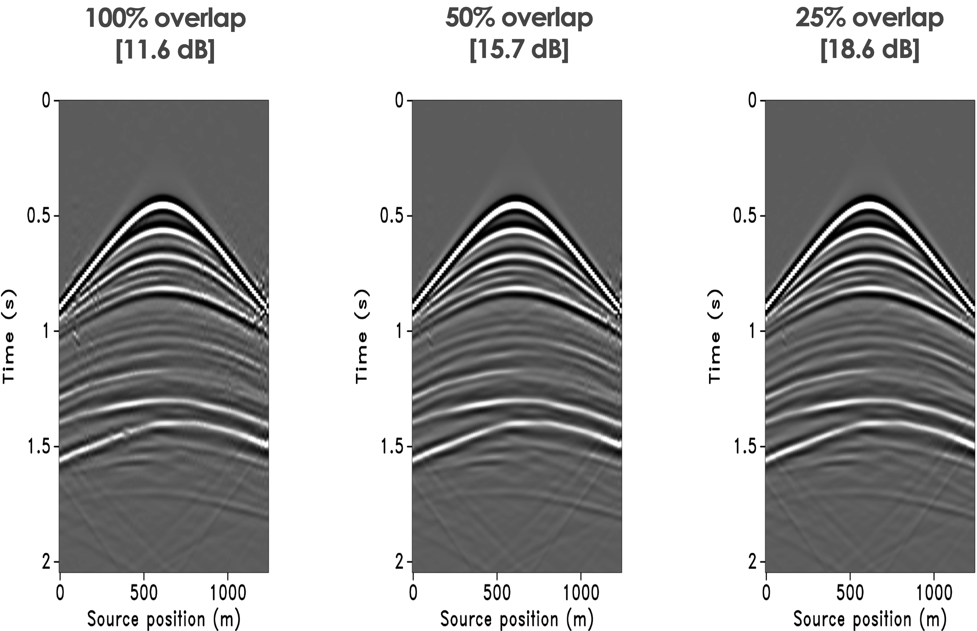
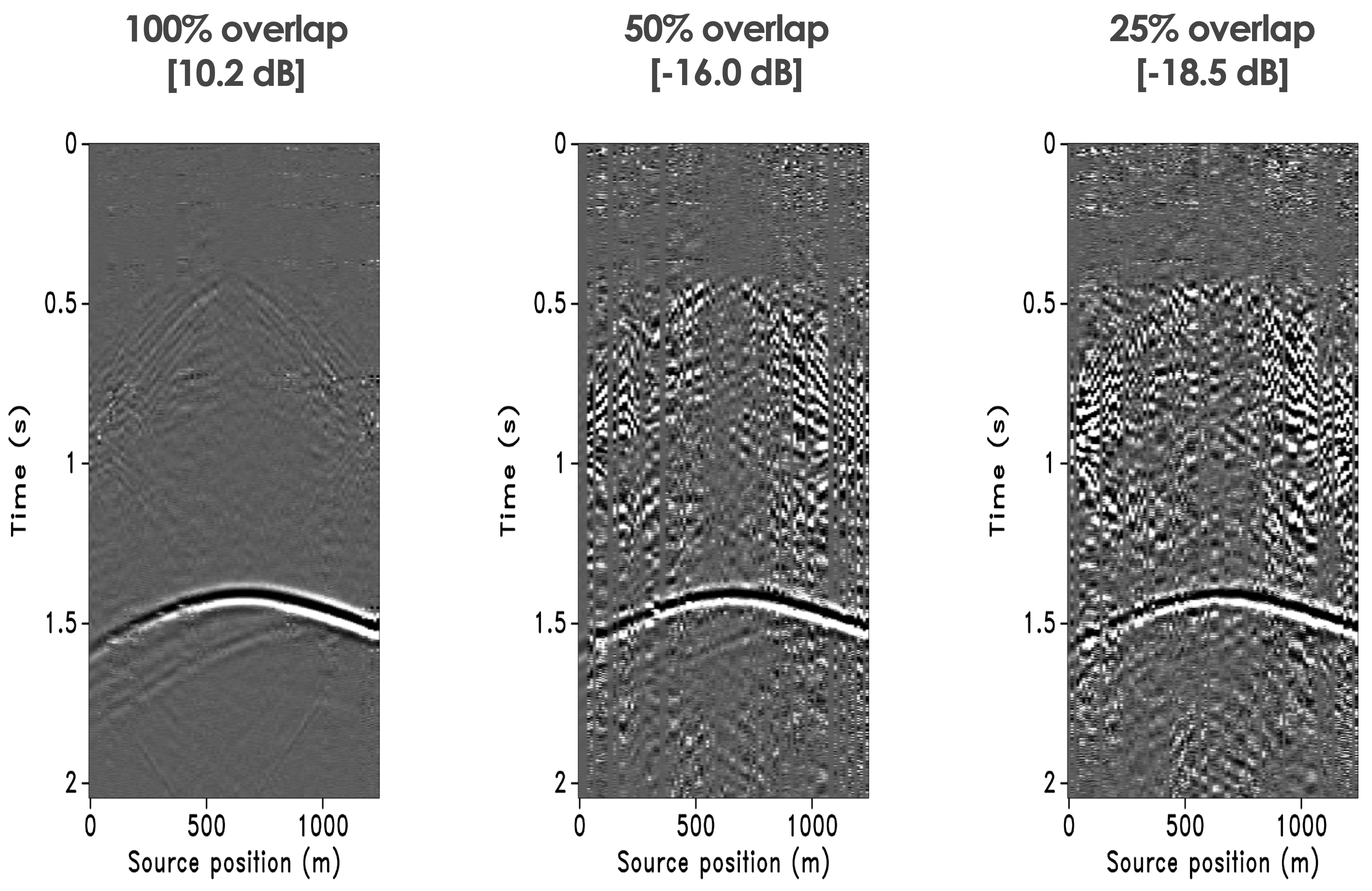
In this scenario, the surveys are exactly replicated when the source positions of the baseline and monitor surveys overlap. The results for independent processing and with the joint recovery model are summarized in Figure 2a and 2b for the baseline and in Figure 3a and 3b for the time-lapse differences. From these results, we observe data (i) the baseline obtained with the joint recovery model improves significantly when the sources do not overlap—i.e., the surveys are not replicated; (ii) the time-lapse differences deteriorate drastically when the surveys are not replicated; and (iii) the time-lapse difference is best when replicated.


Calibrated off-the-grid acquisition
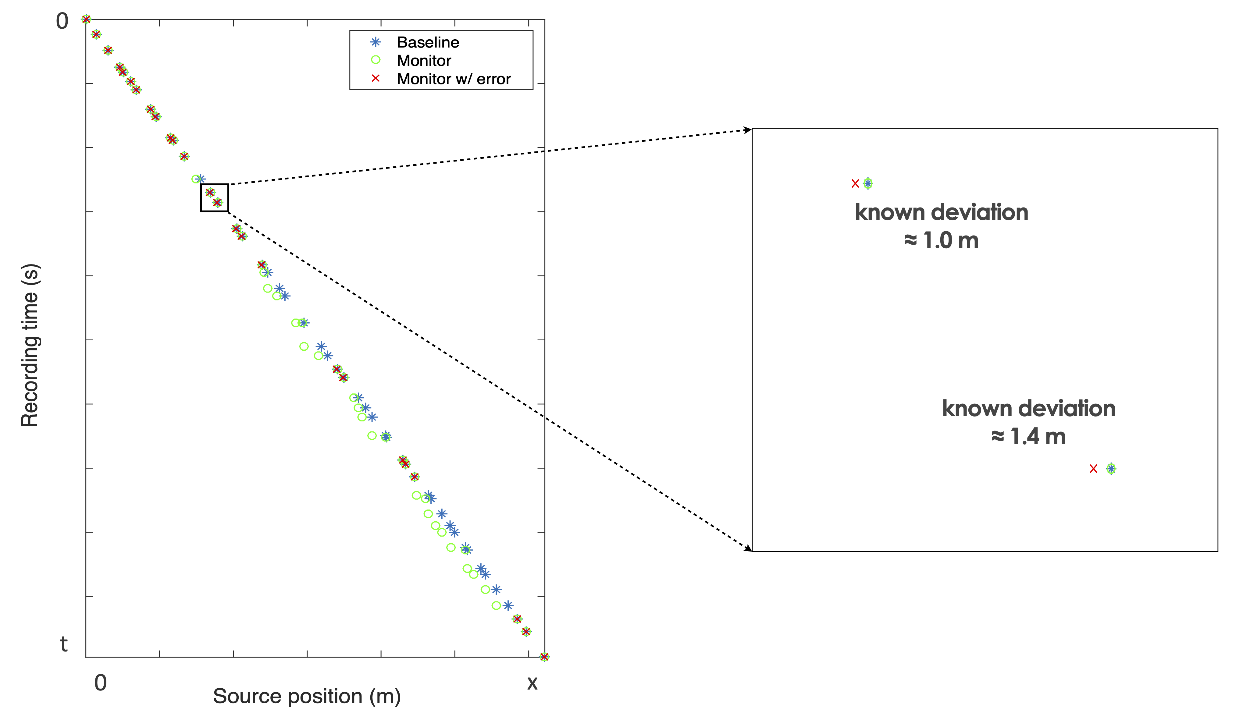
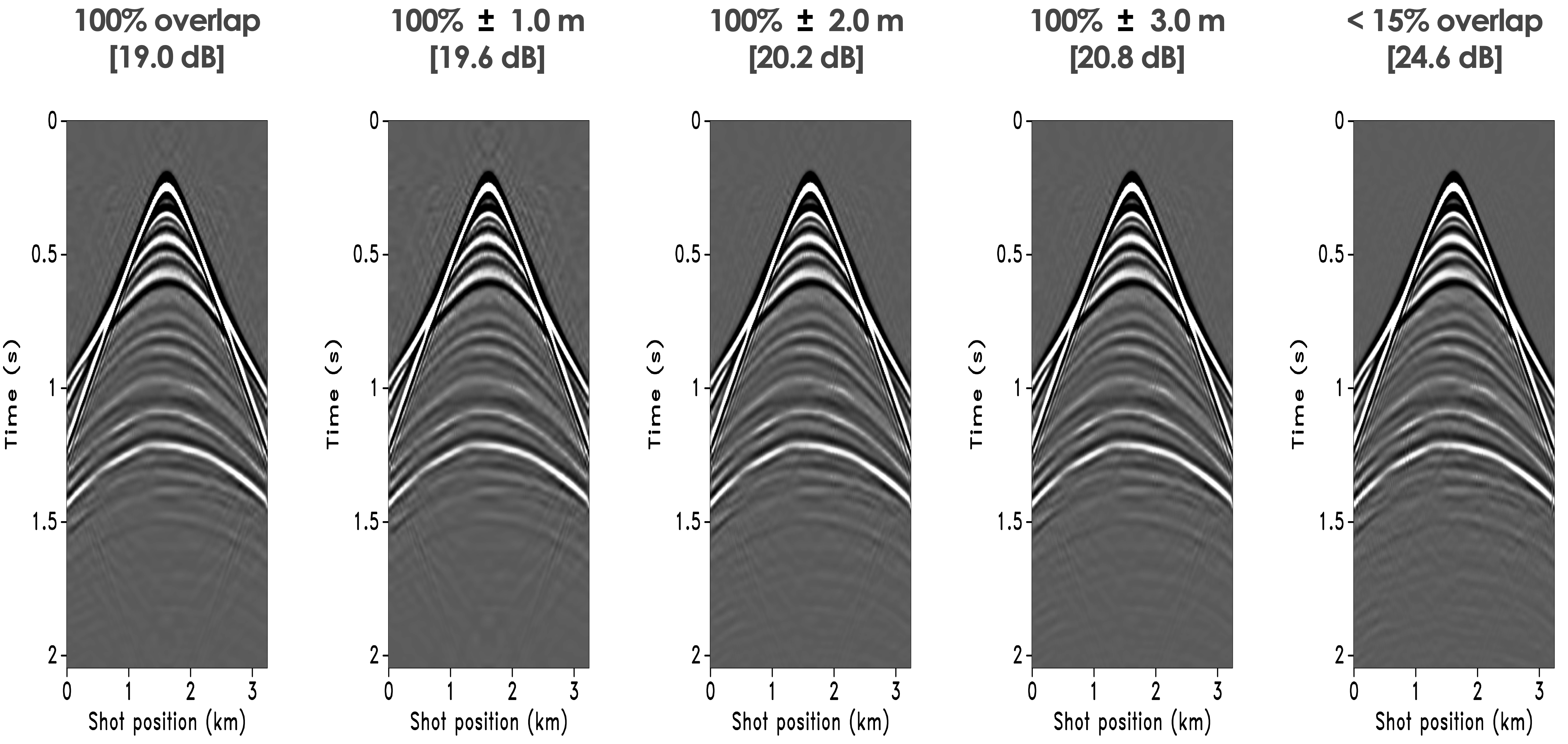
While the on-the-grid results suggest that surveys should be replicated, in practice this can not be achieved since data is always collected off-the-grid—i.e., sampling points never coincide exactly with the spatial locations of a periodic grid. To mimic this more practical situations, we consider off-the-grid acquisition where the post-plot source positions are known to within known small deviations from the periodic grid. See Figure 4. Even though these deviations are small, their impact on the recovery of the baseline and 4D differences is significant as can be observed from Figure 5a for the baseline recovery and Figure 5b for the time-lapse recovery. Both recovery results improve when there are small deviations between the baseline and monitor surveys. Moreover, the results for the baseline improve when the surveys have little overlap—so we effectively do not have to make efforts to replicate the surveys as long as we ensure we are well calibrated. The same observation applies to the 4-D difference so the tentative answer to our questions whether surveys should be replicated is a resounding no.
Non-calibrated off-the-grid acquisition
Even though the conclusion from Calibrated off-the-grid acquisition may have profound implications on how to conduct time-lapse surveys, it relies on perfect calibration both of the source firing times and positions. We ignore timing errors because these are well controlled. We do, however, allow for small random positioning errors that are unknown. For the survey details listed in Table 1, we run experiments for dense off-the-grid surveys and for surveys acquired with Compressive Sensing with \(4\times\) improved acquisition productivity. The results of these experiments are summarized in Figure 6, for an earth without time-lapse changes (top row) and with time-lapse changes (bottom row).
| Conventional dense survey | Low-cost (\(4\times\) compressed) survey | |
|---|---|---|
| Shot geometry | Flip-flop irregular | 2 Sim. source |
| shot sampling | (time-jittered sources) | |
| Receiver geometry | OBC | OBC |
| Number of shots | 450 | 100 |
| Shot interval | 12.5m | 50m |
| Number of receivers | 450 | 450 |
| Receiver interval | 12.5m | 12.5m |
| Recovery (Processing) | Regularization | Shot separation, Interpolation, Regularization |
From these experiments we conclude the following: (i) The signal-to-noise ratio (S/N) and NRMS value are the best for dense surveys when the calibration is perfect. However, the advantage of dense replicated acquisitions disappears when there are small calibration errors (above 10% of the average shot interval); (ii) the S/R and NRMS for the recovery of the time-lapse signal becomes comparable or even better for the joint recovery model for small calibration errors; and (iii) the joint recovery model is more robust to calibration errors leading to NRMS values that remain acceptable.
The joint recovery model for seismic denoising
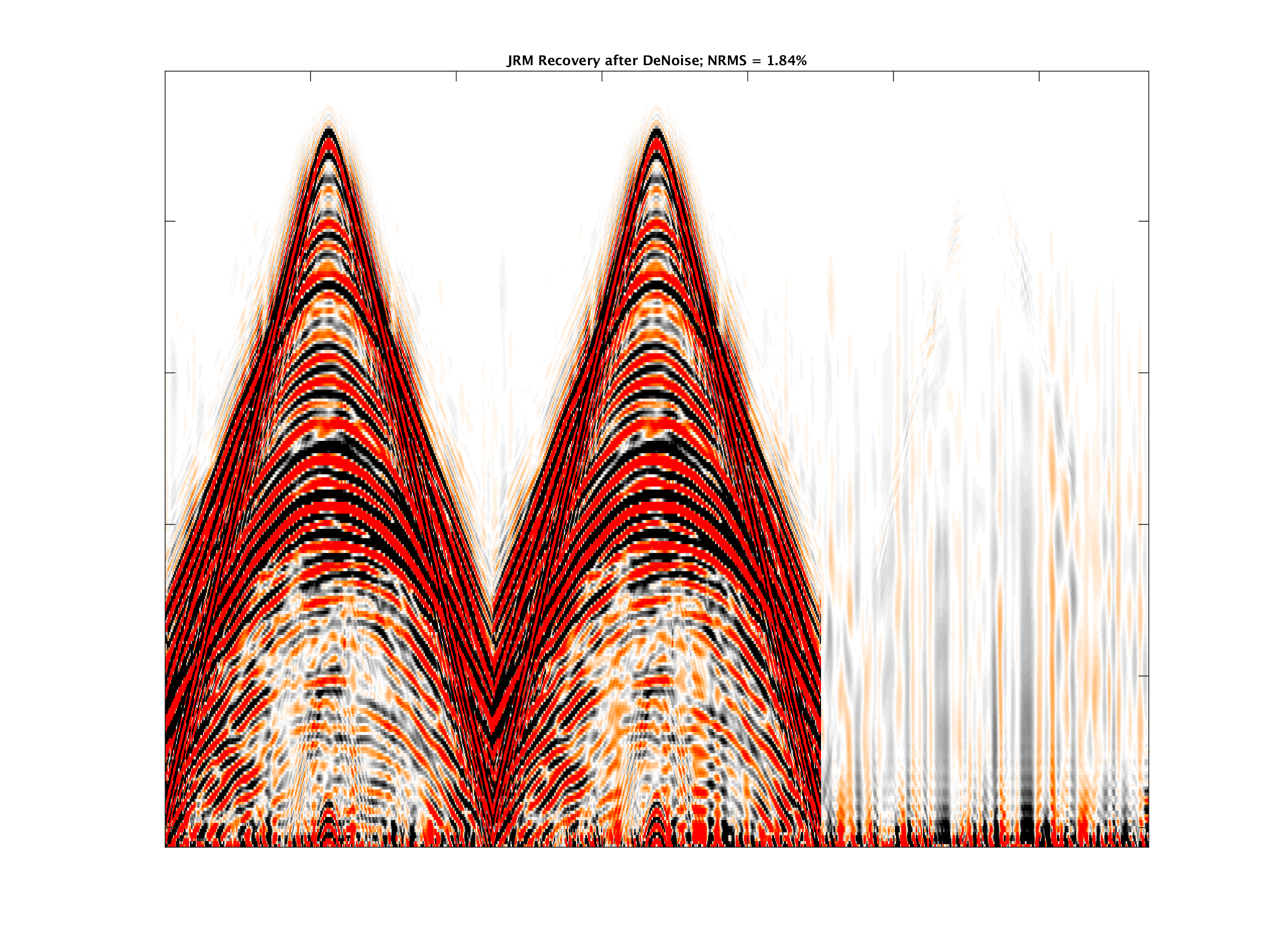
So far, the examples of time-lapse wavefield recovery from randomized (simultaneous) source acquisition were assumed to be noise free. In practice, the noise-free assumption is obviously never met. For this purpose, Oghenekohwo and Herrmann (2017) considered the recovery of time-lapse data corrupted my different realizations of swell noise. To study the effects non-replication, noise, and calibration errors (max error of \(2.5\,\mathrm{m}\)), we consider a fixed-spread seismic data acquisition with ocean bottom receivers and time-jittered overlapping sources for a subsurface model without time-lapse changes. In this situation, any signal within the time-lapse difference gathers is due to the noise and non-replication of the surveys (different source firing times between baseline and monitor surveys. Figure 7 compares independent recovery and joint recovery before and after removing the swell noise with \(f-k\) filtering. The results show that the JRM is able to handle swell noise better, an observation consistent with improves 4D seismic interpretability (Wei et al., 2018) reported by Chevron (Wei et al., 2018; Tian et al., 2018).
The joint recovery model for seismic imaging and inversion
Up to now, the applications of the joint recovery model have been limited to seismic data Processing via sparse inversion producing regular densely sampled data volumes for the baseline and monitor surveys. However, the employment of the joint recovery model can be extended to SPLS-RTM, Full-Waveform Inversion, and Monitoring with multiple monitoring surveys as reported in
- Felix Oghenekohwo and Felix J. Herrmann, “Improved time-lapse data repeatability with randomized sampling and distributed compressive sensing”, in EAGE Annual Conference Proceedings, 2017.
- Felix Oghenekohwo, “Economic time-lapse seismic acquisition and imaging–-Reaping the benefits of randomized sampling with distributed compressive sensing”, The University of British Columbia, Vancouver, 2017. Chapter 5.
- Ziyi Yin, Mathias Louboutin, and Felix J. Herrmann, “Compressive time-lapse seismic monitoring of carbon storage and sequestration with the joint recovery model”, in SEG Technical Program Expanded Abstracts, 2021, pp. 3434-3438.
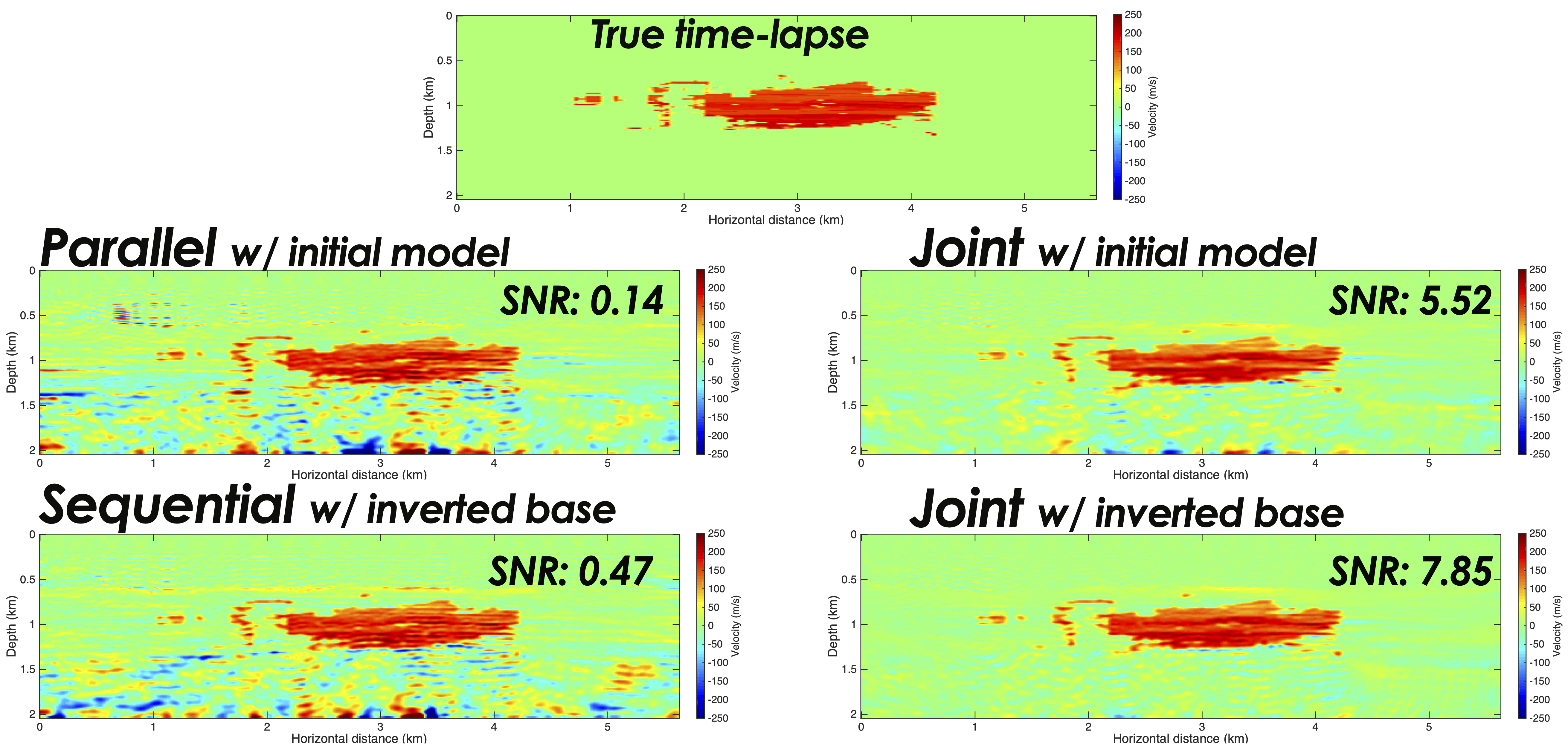
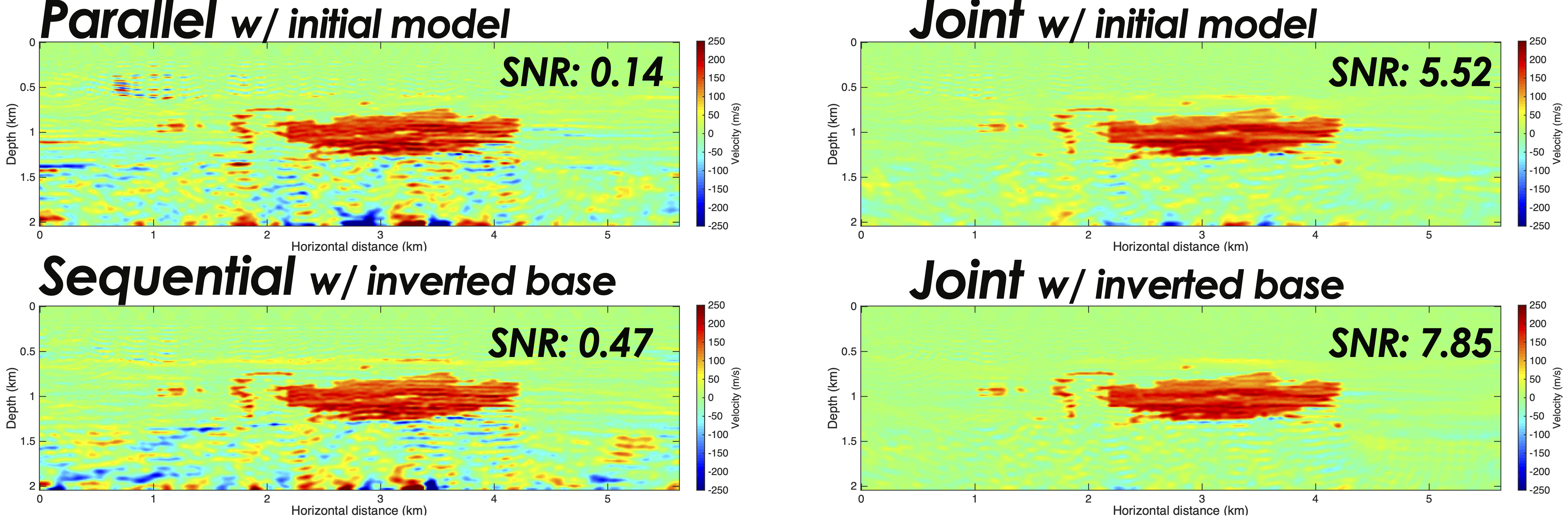
In the near future, we also plan to extend our early findings of applying JRM to sparsity-promoting updates of Full-Waveform Inversion. These findings indicate that significant improvements may be achieved compared to independent as well as sequential inversions during which the time-lapse datasets are either inverted separately or where the baseline inversion is used as a starting model for the monitor inversion. As expected, using the inverted baseline also improves JRM. See Figure 8.
References
Baron, D., Duarte, M. F., Sarvotham, S., Wakin, M. B., and Baraniuk, R. G., 2005, An information-theoretic approach to distributed compressed sensing: In Proc. 45rd conference on communication, control, and computing.
Eggenberger, K., Christie, P., Manen, D.-J. van, and Vassallo, M., 2014, Multisensor streamer recording and its implications for time-lapse seismic and repeatability: The Leading Edge, 33, 150–162.
Herrmann, F. J., and Hennenfent, G., 2008, Non-parametric seismic data recovery with curvelet frames: Geophysical Journal International, 173, 233–248.
Johnston, D. H., 2013, Practical applications of time-lapse seismic data: Society of Exploration Geophysicists.
Landrø, M., 1999, Repeatability issues of 3-d vSP data: Geophysics, 64, 1673–1679.
Lumley, D., and Behrens, R., 1998, Practical issues of 4D seismic reservoir monitoring: What an engineer needs to know: SPE Reservoir Evaluation & Engineering, 1, 528–538.
Oghenekohwo, F., 2017, Economic time-lapse seismic acquisition and imaging-reaping the benefits of randomized sampling with distributed compressive sensing: Master’s thesis,. The University of British Columbia. Retrieved from https://slim.gatech.edu/Publications/Public/Thesis/2017/oghenekohwo2017THetl/oghenekohwo2017THetl.pdf
Oghenekohwo, F., and Herrmann, F. J., 2017, Improved time-lapse data repeatability with randomized sampling and distributed compressive sensing: EAGE annual conference proceedings. doi:10.3997/2214-4609.201701389
Oghenekohwo, F., Wason, H., Esser, E., and Herrmann, F. J., 2017, Low-cost time-lapse seismic with distributed compressive sensing-part 1: Exploiting common information among the vintages: Geophysics, 82, P1–P13. doi:10.1190/geo2016-0076.1
Tian, Y., Wei, L., Li, C., Oppert, S., and Hennenfent, G., 2018, Joint sparsity recovery for noise attenuation: In SEG technical program expanded abstracts 2018 (pp. 4186–4190). Society of Exploration Geophysicists.
Wason, H., Oghenekohwo, F., and Herrmann, F. J., 2017, Low-cost time-lapse seismic with distributed compressive sensing-part 2: Impact on repeatability: Geophysics, 82, P15–P30. doi:10.1190/geo2016-0252.1
Wei, L., Tian, Y., Li, C., Oppert, S., and Hennenfent, G., 2018, Improve 4D seismic interpretability with joint sparsity recovery: In SEG technical program expanded abstracts 2018 (pp. 5338–5342). Society of Exploration Geophysicists.