Acquisition

Introduction

Due to recent advances in compressive sensing (Candès et al., 2006), seismic data is gathered randomly to increase acquisition productivity (C. Mosher et al., 2014a; Kumar et al., 2015a; Chiu, 2019). Wavefield reconstruction aims to recover fully sampled data from subsampled seismic observations (Hennenfent and Herrmann, 2008; Kumar et al., 2015a; Zhang et al., 2020). Gilles (2008) proposed jittered subsampling to remove the imprint of large gaps in uniform random sampling. By controlling the maximum gap size of subsampled data, jittered subsampling creates favorable conditions for seismic wavefield recovery based on sparsity promotion in a domain of localized atoms such as curvelets (Herrmann et al., 2008). While uniform random (Candès and Recht, 2009; Candès and Tao, 2010) and random jittered (Herrmann et al., 2008) subsampling schemes are easy to generate, they are suboptimal and can be improved by solving certain optimization problems (C. Mosher et al., 2014a; Manohar et al., 2018; Li et al., 2017). Although these techniques have yielded promising results, they require either extensive computational resources to determine the optimal source-receiver layout using simulations (C. Mosher et al., 2014a), or a thorough understanding of the to-be-recovered seismic data (Manohar et al., 2018; Guo and Sacchi, 2020). In order to improve the quality of a given randomized subsampling mask, we propose a simulation-free seismic survey design that iteratively increases the spectral gap of the subsampling mask, a characteristic recently associated with reconstruction quality Matrix Completion (Bhojanapalli and Jain, 2014, López et al. (2022)).

Aside from automatic generation of optimized sampling masks, SLIM has worked extensively on the development of Compressive Sensing techniques for simultaneous source acquisition e.g. via Time-jittered, blended marine acquisition. Other key references on our Acquisition and wavefield reconstruction via Sparsity promotion and Matrix Completion work include

• Hassan Mansour, Haneet Wason, Tim T.Y. Lin, and Felix J. Herrmann, “Randomized marine acquisition with compressive sampling matrices”, Geophysical Prospecting, vol. 60, p. 648-662, 2012.
• Rajiv Kumar, Haneet Wason, and Felix J. Herrmann, “Source separation for simultaneous towed-streamer marine acquisition –- a compressed sensing approach”, Geophysics, vol. 80, p. WD73-WD88, 2015.
• Rajiv Kumar, Curt Da Silva, Okan Akalin, Aleksandr Y. Aravkin, Hassan Mansour, Ben Recht, and Felix J. Herrmann, “Efficient matrix completion for seismic data reconstruction”, Geophysics, vol. 80, p. V97-V114, 2015.
• Rajiv Kumar, Shashin Sharan, Haneet Wason, and Felix J. Herrmann, “Time-jittered marine acquisition–-a rank-minimization approach for 5D source separation”, in SEG Technical Program Expanded Abstracts, 2016, p. 119-123.
• Curt Da Silva and Felix J. Herrmann, “Optimization on the Hierarchical Tucker manifold - applications to tensor completion”, Linear Algebra and its Applications, vol. 481, p. 131-173, 2015.
• Aleksandr Y. Aravkin, Rajiv Kumar, Hassan Mansour, Ben Recht, and Felix J. Herrmann, “Fast methods for denoising matrix completion formulations, with applications to robust seismic data interpolation”, SIAM Journal on Scientific Computing, vol. 36, p. S237-S266, 2014.

Simulation-free seismic survey design

A number of effective algorithms for reconstructing subsampled seismic data have been developed to lower the cost of seismic data acquisition. These technologies record as little information as possible in the field while reconstructing wavefields in unrecorded regions. Matrix completion is a relative simple and efficient method to implement wavefield reconstruction. Here is an illustration of reconstructing data collected from Gulf of Suez.

More details of matrix completion can be found in this page.

Designing randomized subsampling masks enables accurate wavefield reconstruction through matrix completion techniques (Bhojanapalli and Jain, 2014, López et al. (2022)). Motivated by these findings, we propose the following simulation-free seismic survey design. Given \(n_s\) source locations, \(n_r\) receiver locations, and the source subsampling ratio \(r\), we propose to solve a non-convex combinatorial optimization problem with respect to the subsampling mask \(\mathbf M \in \{0,1\}^{n_s \times n_r}\)—i.e., we have \[ \begin{equation} \begin{aligned} \min_{\mathbf{M}}\; & \frac {\sigma_2(\mathcal{A}( \mathbf{M} ))}{\sigma_1(\mathcal{A}(\mathbf{M}))} \\ \text{s.t.}\; & \|\mathbf{M}\|_0 = \lfloor n_s \times r\rfloor \times n_r \cap \mathbf{M} \in \mathcal{S} \cap \mathbf{M} \in \{0,1\}^{n_s \times n_r}, \end{aligned} \label{SG_opt_1V} \end{equation} \] in which, the objective function consists of the spectral ratio (SR) (López et al. (2022)), defined by the ratio of the first, \(\sigma_1 (\cdot)\), and second, \(\sigma_2 (\cdot)\), singular values. \(\mathcal A\) stands for the transformation operator with seismic reciprocity (Fenati and Rocca, 1984) from the source-receiver domain to the midpoint-offset domain. We constrain the solution to conserve the subsampling ratio (\(\|\mathbf{M}\|_0 = \lfloor n_s \times r\rfloor \times n_r \)) . \(\mathcal{S}\) is a set of all possible subsampling acquisitions that satisfy certain physical constraints.

We initialize the optimization with a jittered subsampling mask with a subsampling ratio of \(r=20\%\) then solve the proposed problem to optimize the SR in the midpoint-offset domain. After reducing the SR of a given mask by \(30\%\), we use the SR optimized mask to observe subsampled data and reconstruct the full data via matrix completion. We compare this result with the original jittered subsampling mask.

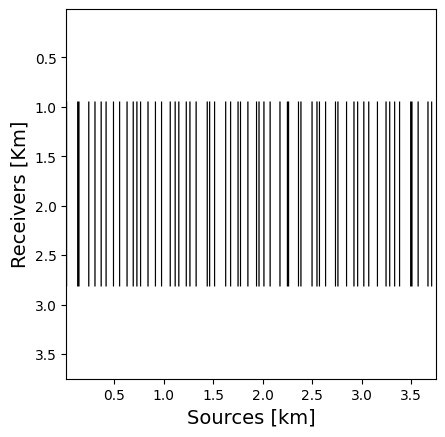
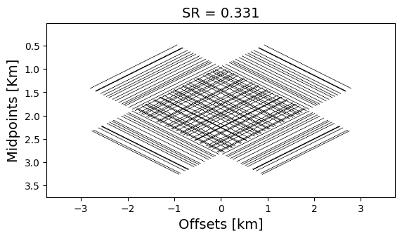
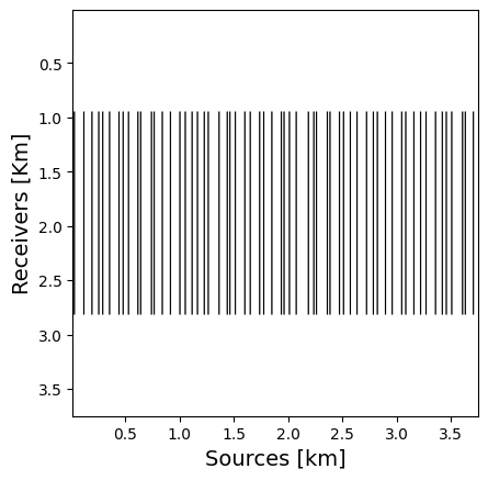
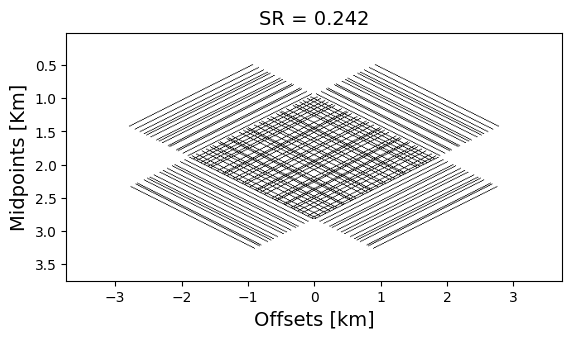
It can be seen from the difference in Slider 2 that the proposed subsampling data reconstruction contains less signal residual than the jittered one. These experiments have led us to the conclusion that the proposed method produces the optimal subsampling mask for wavefield reconstruction based on matrix completion.

Additional information on the subject is provided in this presentation and this SEG2022 abstract. Code of this application is provided here.

Compressive Marine Acquisition

At SLIM, we looked extensively in improving acquisition productivity using techniques from Compressive Sensing. For Marine acquisition, this amounted to considering both static, e.g. OBC/OBN or PRM (Wason et al., 2017), and cheaper dynamic towed-array acquisition (Kumar et al., 2015b). Since vessel time is a cost consideration, we considered both static and dynamic randomized source subsampling as illustrated in Figure 2 below.

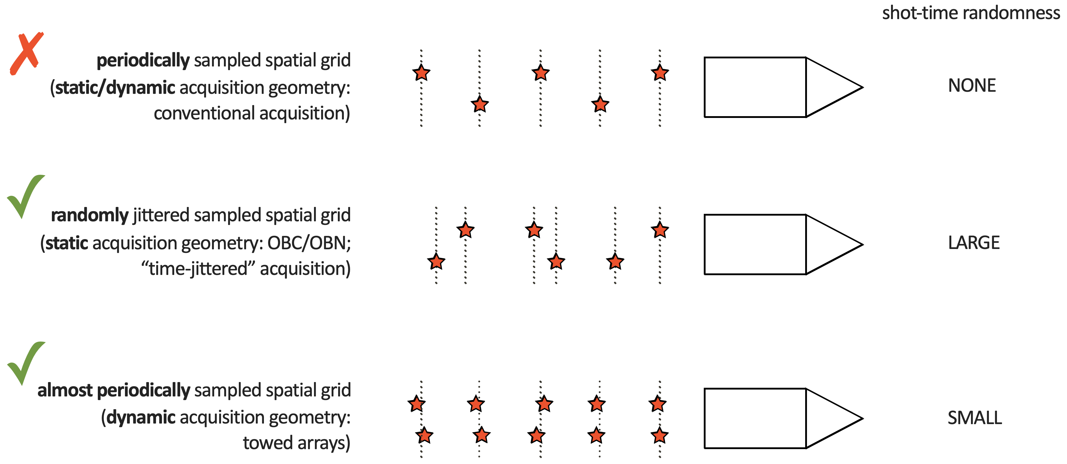
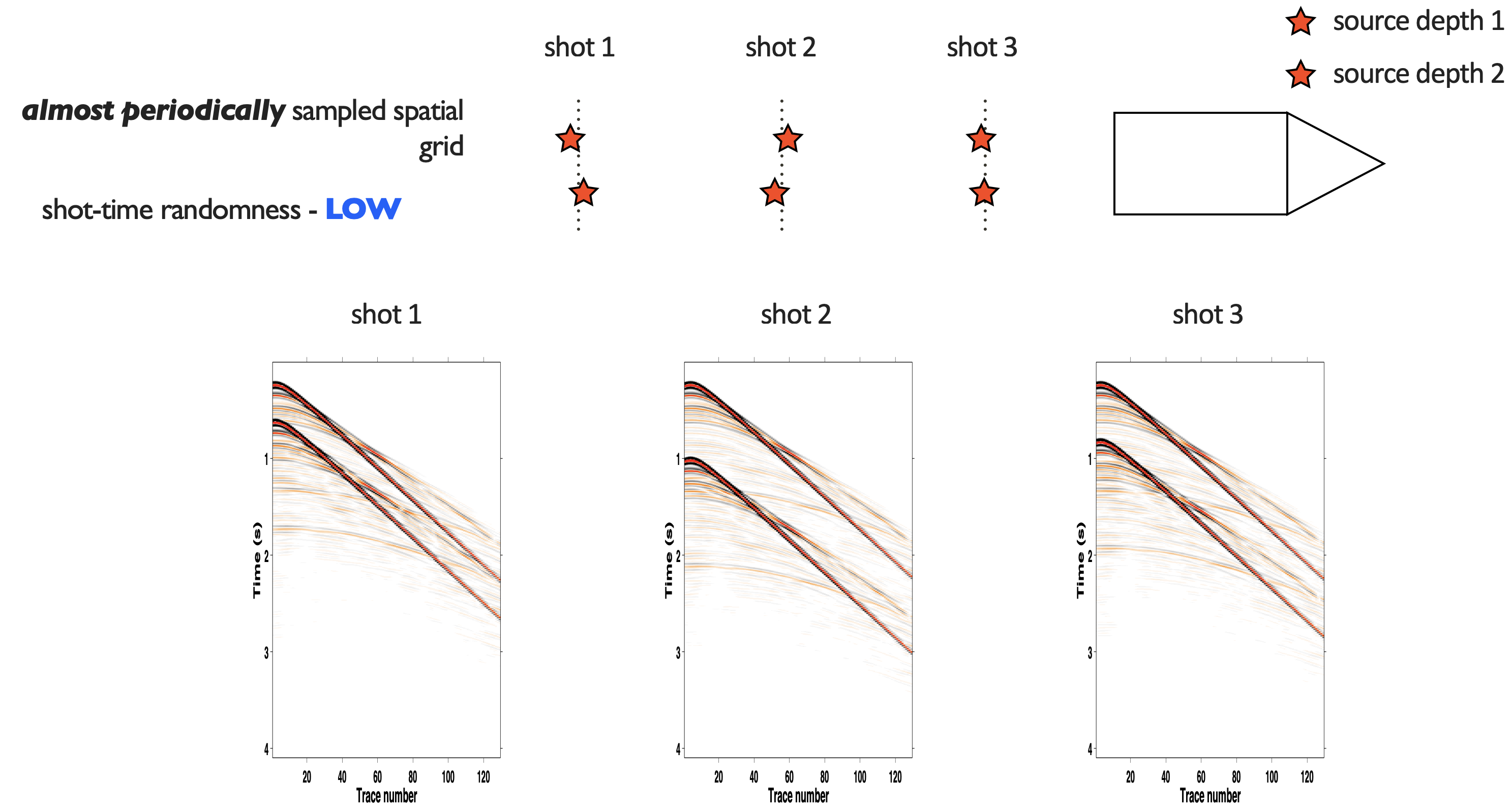
Because the source subsampling leads to overlap in observed shot records we observed that acquisitions with randomized source firing times would perform best. For static acquisitions, we obtained the best results for large variations in the source firing times while movement in the towed arrays calls for small randoms and the use of over/under shooting.

Time-jittered blended marine acquisition¹

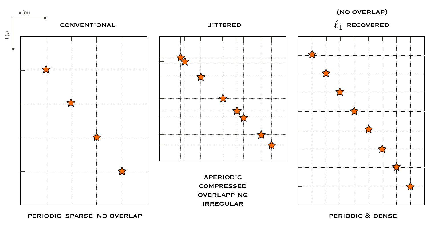
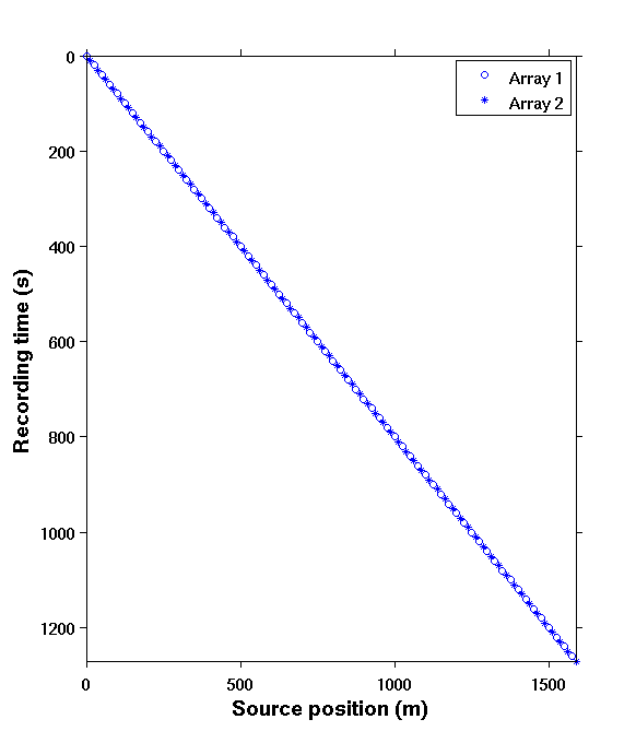
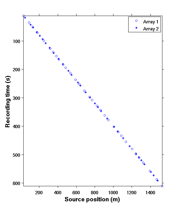
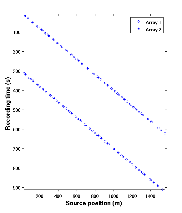
In principle, blended acquisition involves firing multiple sources at randomly-jittered times, resulting in overlaps between shot records. In contrast, conventional (sequential) acquisition has no overlaps between shot records as the source vessel fires at regular times, which translates to regular spatial locations for a given speed. Blended acquisition improves the productivity and efficiency of acquisition surveys (Beasley, 2008; Berkhout, 2008; C. Mosher et al., 2014b). However, the challenge with such schemes is to deblend the acquired data since many processing techniques, such as SRME, EPSI, RTM, FWI, etc., require full (regular) sampling. Figure 5 illustrates the conventional and jittered marine acquisition schemes.

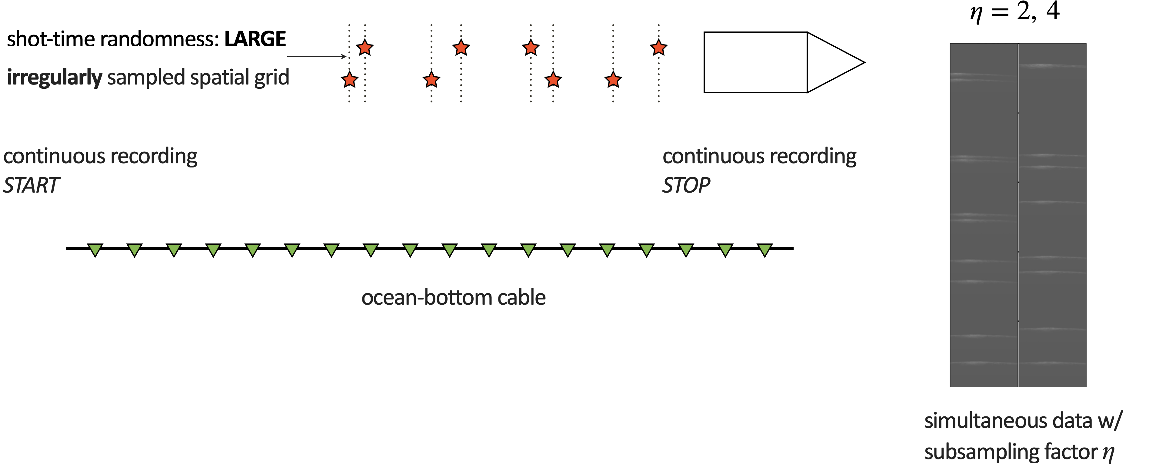
Our approach is two-fold: i) design of time-jittered, blended acquisition scheme, and ii) deblending by curvelet-domain sparsity promotion using \(\ell_1\) constraints. What we aim to achieve with this approach is outlined in Figure 4. Wason and Herrmann (2013) successfully adapted this approach to single- and multiple-vessel, time-jittered (ocean bottom) acquisition, wherein airguns fire at randomly-jittered times that translate to randomly-jittered spatial locations for a given speed, with the receivers (ocean bottom cables/nodes) recording continuously.

Deblending by sparse inversion via one-norm minimization

We formulate the deblending problem as a basis persuit (BP) optimization problem \[ \begin{equation} \tag{BP} \min\limits_{\vector{x} \in \mathbb{C}^P} \|\vector{x}\|_1 \quad \textrm{subject to} \quad \vector{y} = \vector{Ax}, \label{BP} \end{equation} \] which aims to solve a linear system of underdetermined equations \(\vector{y} = \vector{Ax}\), where \(\vector{y} \in \mathbb{C}^n\) represents the randomly undersampled and blended measurements with \(n \ll N\), where \(N\) is the ambient dimension of the data. The vector \(\vector{x}\) represents a compressible representation of seismic data in a sparsifying domain, \(\vector{S}\). The measurement matrix \(\vector{A}\) is a combination of a sampling matrix (\(\vector{M}\)), and the sparsifying transform, such that, \(\vector{A} = \vector{MS^H}\). A seismic line with \(N_s\) sources, \(N_r\) receivers, and \(N_t\) time samples can be reshaped into an \(N\) dimensional vector \(\vector{f}\), where \(N = N_s \times N_r \times N_t\). Given the measurements \(\vector{y} = \vector{Mf}\), the aim is to recover a sparse approximation \(\vector{\tilde{f}}\) (= \(\vector{S^H} \tilde{\vector{x}}\)) by solving the \(\ref{BP}\) problem using the SPG\(\ell_1\) solver (Van Den Berg and Friedlander, 2008). We use curvelets as the sparsifying basis. For more details, also see Sparse recovery under Compressive Sensing.

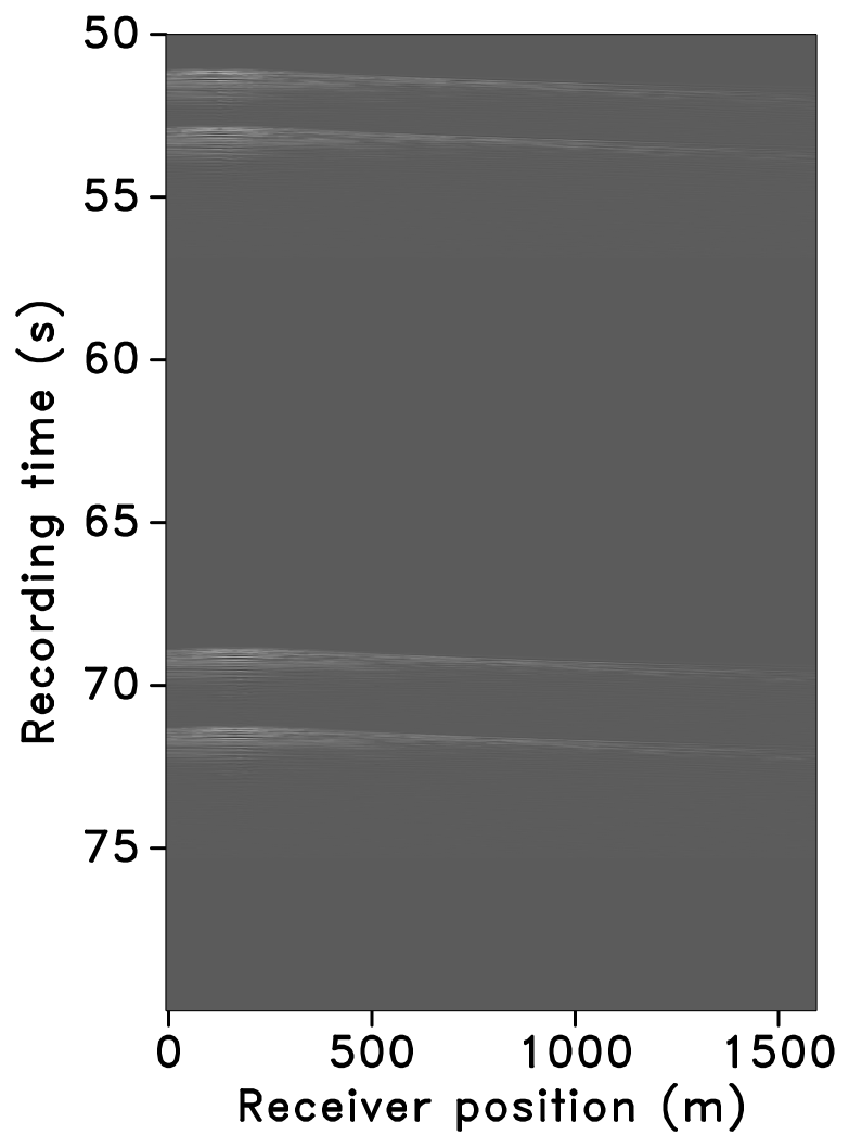
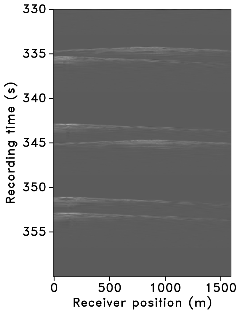
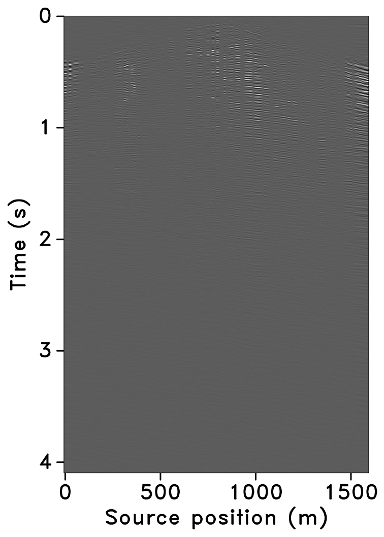
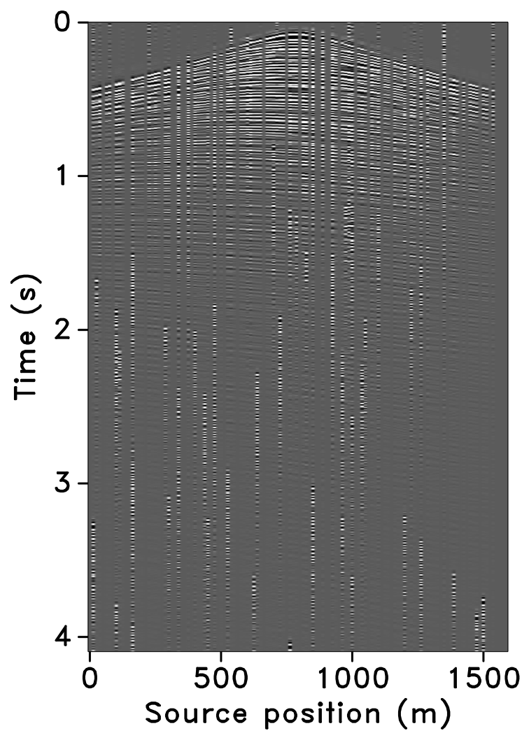
The time-jittered blended acquisition is simulated on a 2-D seismic line from the Gulf of Suez, with one and two source vessels. Figures 6a and 6b show the corresponding randomly undersampled and blended measurements for the two surveys. Note that only 30 seconds of the continuously recorded data is shown. If we simply apply the adjoint of the acquisition operator to the blended data—i.e., \(\vector{M}^H\vector{y}\), the interferences (or source crosstalk) due to overlaps in the shot records appear as random noise—i.e., incoherent and non-sparse, in the common-receiver domain, as illustrated in Figures 7a and 8a. The overlap between shot records appears in the common-shot domain (Figures 7d and 8d).

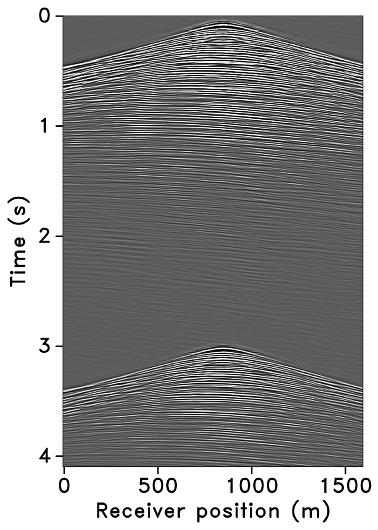
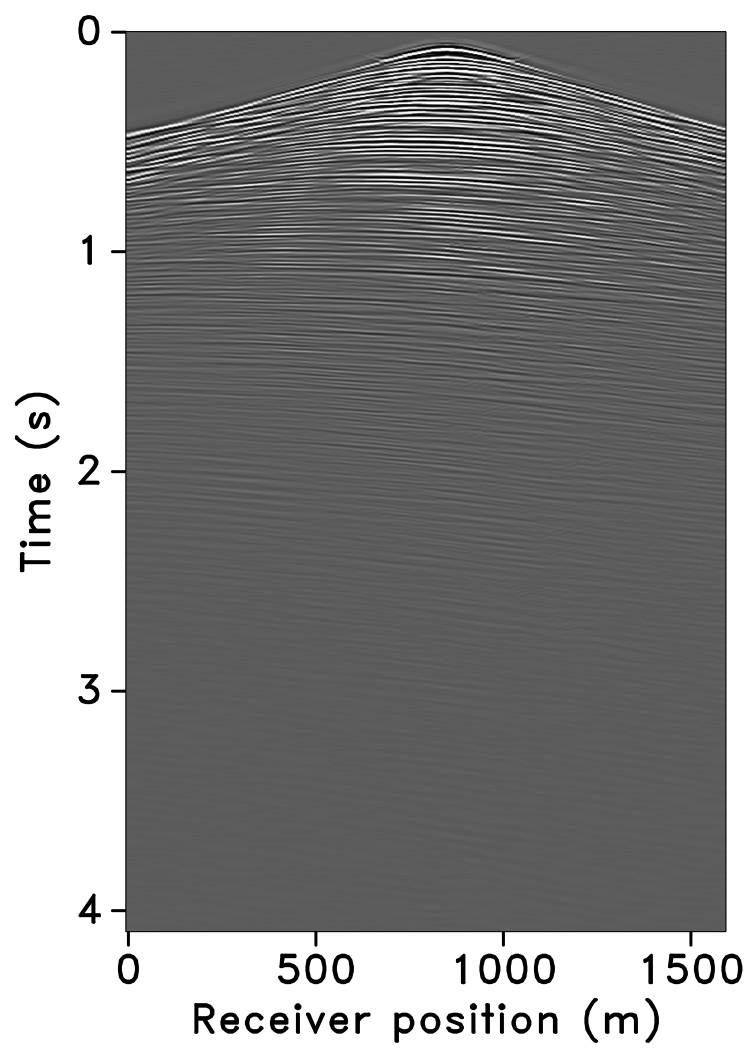
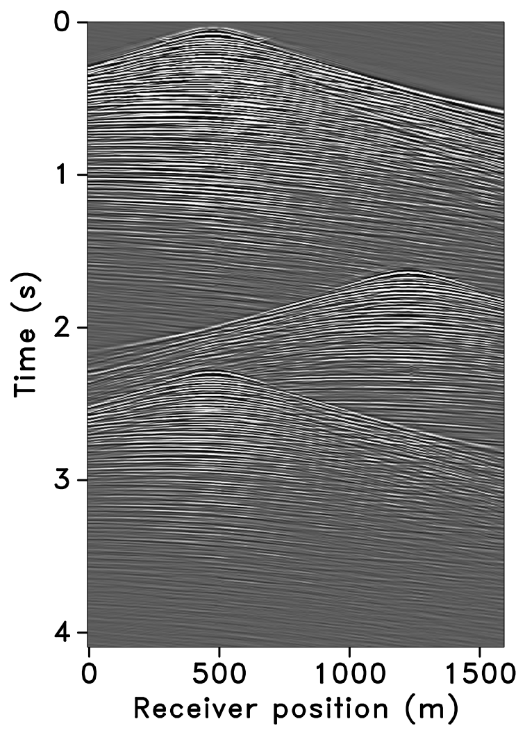
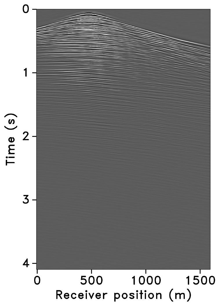
Our goal, however, is to recover the conventional, unblended shot records from the blended data by working with the entire (blended) data volume, and not on a shot-by-shot basis. For acquisition with one source vessel, the undersampling factor, \(\eta = 2\), hence, the recovery problem becomes a joint deblending and interpolation problem. For acquisition with two source vessels, the recovery problem is a deblending problem alone. Recovery via curvelet-based sparsity-promotion for both scenarios is shown in Figures 7 and 8.

Software implementation

Software for this application is provided here. Julia implementation for this application will be provided here.

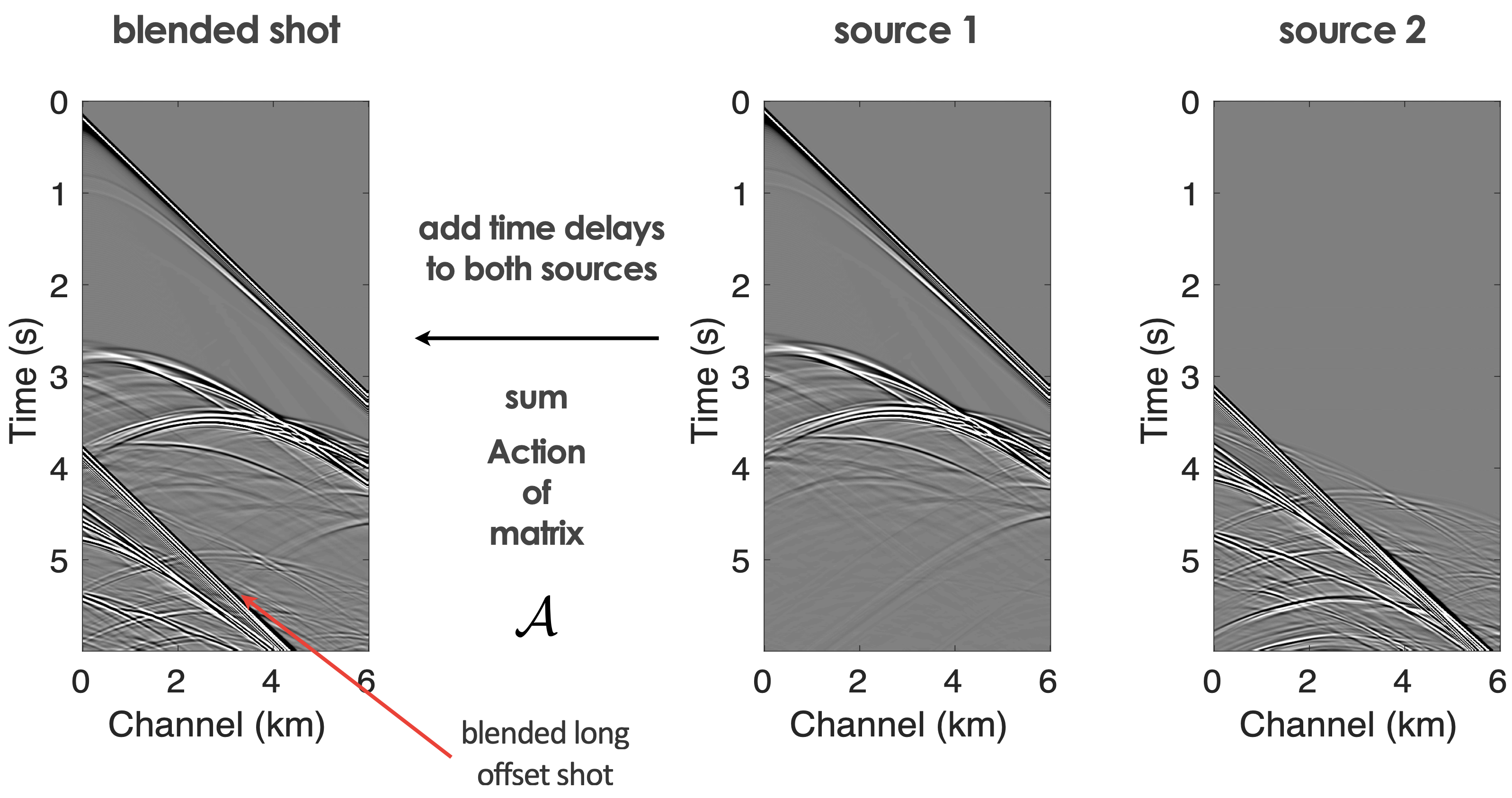
Source separation for simultaneous towed-streamer marine acquisition²

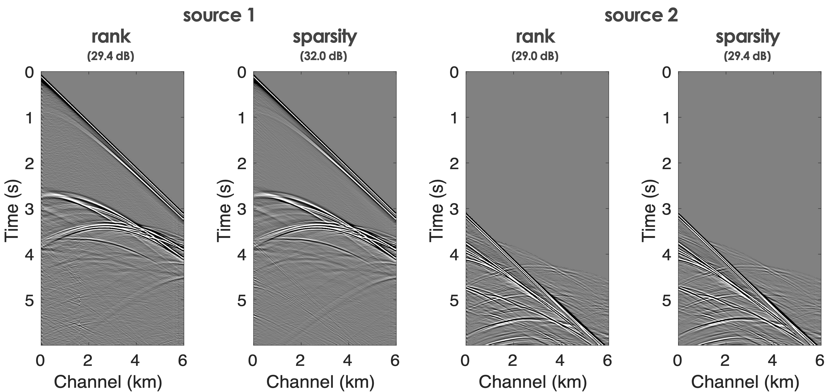
To handle dynamic towed-array acquisition, we considered the use of Sparsity promotion and Matrix completion techniques to separate blended shots as depicted in Figure 9 and deblending results using Sparsity promotion and Matrix completion techniques aimed at inverting the respective blending operators \[ \begin{equation} \begin{aligned} \overbrace{ \begin{bmatrix} {{\mathbf{MT_1}}}{\bf{\mathbf{S}}}^H & {{\mathbf{MT_2}}}{\bf{\mathbf{S}}}^H \end{bmatrix} }^{\mathbf{A}} \overbrace{ \begin{bmatrix} {\mathbf{x}}_1 \\ {\mathbf{x}}_2 \end{bmatrix} }^{\mathbf{x}} = {\mathbf{b}} \end{aligned} \label{matrix} \end{equation} \] and \[ \begin{equation*} \begin{aligned} \overbrace{ \begin{bmatrix} {{\mathbf{M}}{\mathbf{T}}_1}{\bf{\mathcal{S}}}^H & {{\mathbf{M}}{\mathbf{T}}_2}{\bf{\mathcal{S}}}^H \end{bmatrix} }^{\mathcal{A}} \overbrace{ \begin{bmatrix} {{\mathbf{X}}}_1 \\ {{\mathbf{X}}}_2 \end{bmatrix} }^{{\mathbf{X}}} = {{\mathbf{b}}} , \end{aligned} \end{equation*} \] where \({\mathbf{T}}_1\) and \({\mathbf{T}}_2\) represent the firing-time delays operators, which apply uniformly random time delays, and where \(\mathbf{S}\) and \(\mathcal{S}\) are the curvelet and rank revealing (mid-point offset) transform operators and \(\mathbf{x}_{1,2}\) and \(\mathbf{X}_{1,2}\) the deblended shot records organized as a vector in the curvelet domain or as a matrix in the mid-point offset domain (Kumar et al., 2015b). The latter are computed via \[ \begin{equation} \underset{\mathbf{X}}{\text{minimize}} \quad \|\mathbf{X}\|_* \quad \text{subject to} \quad \|\mathcal{A} ({\mathbf{X}}) - {\mathbf{b}}\|_2 \leq \epsilon, \tag{BPDN$_\epsilon$} \label{BPDNepsilon} \end{equation} \] with \(\left\| {\mathbf{X}}\right\|_* = \|\sigma\|_1\) the nuclear norm and \(\epsilon\) some tolerance.

Check Monitoring, for Time-lapse seismic and Geological Carbon Storage.

References

Beasley, C. J., 2008, A new look at marine simultaneous sources: The Leading Edge, 27, 914–917. doi:10.1190/1.2954033
Berkhout, A. J. `., 2008, Changing the mindset in seismic data acquisition: The Leading Edge, 27, 924–938. doi:10.1190/1.2954035
Bhojanapalli, S., and Jain, P., 2014, Universal matrix completion: In International conference on machine learning (pp. 1881–1889). PMLR.
Candès, E. J., and Recht, B., 2009, Exact matrix completion via convex optimization: Foundations of Computational Mathematics, 9, 717–772.
Candès, E. J., and Tao, T., 2010, The power of convex relaxation: Near-optimal matrix completion: IEEE Transactions on Information Theory, 56, 2053–2080.
Candès, E. J., Romberg, J., and Tao, T., 2006, Robust uncertainty principles: Exact signal reconstruction from highly incomplete frequency information: IEEE Transactions on Information Theory, 52, 489–509.
Chiu, S. K., 2019, 3D attenuation of aliased ground roll on randomly undersampled data: In SEG international exposition and annual meeting. OnePetro.
Fenati, D., and Rocca, F., 1984, Seismic reciprocity field tests from the italian peninsula: Geophysics, 49, 1690–1700.
Gilles, H., 2008, Sampling and reconstruction of seismic wavefields in the curvelet domain: PhD thesis,. University of British Columbia.
Guo, Y., and Sacchi, M. D., 2020, Data-driven time-lapse acquisition design via optimal receiver-source placement and reconstruction: In SEG technical program expanded abstracts 2020 (pp. 66–70). Society of Exploration Geophysicists.
Hennenfent, G., and Herrmann, F. J., 2008, Simply denoise: Wavefield reconstruction via jittered undersampling: Geophysics, 73, V19–V28.
Herrmann, F. J., Wang, D., Hennenfent, G., and Moghaddam, P. P., 2008, Curvelet-based seismic data processing: A multiscale and nonlinear approach: Geophysics, 73, A1–A5.
Kumar, R., Da Silva, C., Akalin, O., Aravkin, A. Y., Mansour, H., Recht, B., and Herrmann, F. J., 2015a, Efficient matrix completion for seismic data reconstruction: Geophysics, 80, V97–V114.
Kumar, R., Wason, H., and Herrmann, F. J., 2015b, Source separation for simultaneous towed-streamer marine acquisition—A compressed sensing approach: Geophysics, 80, WD73–WD88.
Li, C., Kaplan, S. T., Mosher, C. C., Brewer, J. D., and Keys, R. G., 2017, Compressive sensing:. Google Patents.
López, O., Kumar, R., Moldoveanu, N., and Herrmann, F., 2022, Graph spectrum based seismic survey design: ArXiv Preprint ArXiv:2202.04623.
Manohar, K., Brunton, B. W., Kutz, J. N., and Brunton, S. L., 2018, Data-driven sparse sensor placement for reconstruction: Demonstrating the benefits of exploiting known patterns: IEEE Control Systems Magazine, 38, 63–86.
Mosher, C., Li, C., Morley, L., Ji, Y., Janiszewski, F., Olson, R., and Brewer, J., 2014a, Increasing the efficiency of seismic data acquisition via compressive sensing: The Leading Edge, 33, 386–391.
Mosher, C., Li, C., Morley, L., Ji, Y., Janiszewski, F., Olson, R., and Brewer, J., 2014b, Increasing the efficiency of seismic data acquisition via compressive sensing: The Leading Edge, 33, 386–391. doi:10.1190/tle33040386.1
Van Den Berg, E., and Friedlander, M. P., 2008, Probing the pareto frontier for basis pursuit solutions: SIAM Journal on Scientific Computing, 31, 890–912.
Wason, H., and Herrmann, F. J., 2013, Time-jittered ocean bottom seismic acquisition: SEG technical program expanded abstracts. doi:10.1190/segam2013-1391.1
Wason, H., Oghenekohwo, F., and Herrmann, F. J., 2017, Low-cost time-lapse seismic with distributed compressive sensing-part 2: Impact on repeatability: Geophysics, 82, P15–P30. doi:10.1190/geo2016-0252.1
Zhang, Y., Sharan, S., Lopez, O., and Herrmann, F. J., 2020, Wavefield recovery with limited-subspace weighted matrix factorizations: In SEG international exposition and annual meeting. OnePetro.