A stochastic quasi-Newton McMC method for uncertainty quantification of full-waveform inversion

In this work we propose a stochastic quasi-Newton Markov chain Monte Carlo (McMC) method to quantify the uncertainty of full-waveform inversion (FWI). We formulate the uncertainty quantification problem in the framework of the Bayesian inference, which formulates the posterior probability as the conditional probability of the model given the observed data. The Metropolis-Hasting algorithm is used to generate samples satisfying the posterior probability density function (pdf) to quantify the uncertainty. However it suffers from the challenge to construct a proposal distribution that simultaneously provides a good representation of the true posterior pdf and is easy to manipulate. To address this challenge, we propose a stochastic quasi-Newton McMC method, which relies on the fact that the Hessian of the deterministic problem is equivalent to the inverse of the covariance matrix of the posterior pdf. The l-BFGS (limited-memory Broyden–Fletcher–Goldfarb–Shanno) Hessian is used to approximate the inverse of the covariance matrix efficiently, and the randomized source sub-sampling strategy is used to reduce the computational cost of evaluating the posterior pdf and constructing the l-BFGS Hessian. Numerical experiments show the capability of this stochastic quasi-Newton McMC method to quantify the uncertainty of FWI with a considerable low cost.

Introduction

Uncertainty is present in each procedure of seismic exploration, from acquisition to modeling and processing. Because of this, quantifying the uncertainty of inversion results has become increasingly important in order to inform decisions in industry. Traditionally, the uncertainty can be quantified in the framework of Bayesian inference, which formulates the posterior probability distribution \(\rho_{\post}(\v)\) of the velocity model \(\mathbf{v}\) as the conditional probability \(\rho(\v|\d_{\obs})\) of the velocity given the observed data \(\d_{\obs}\). The conditional probability \(\rho(\v|\d_{\obs})\) is proportional to the product of the prior on the model \(\rho_{\prior}(\v)\) and the probability of the observed data given the model \(\rho(\d_{\obs}|\v)\) – i.e., we have: \[ \begin{equation} \label{Bayesian} \rho_{\text{post}}(\mathbf{v}) = \rho({\mathbf{v}|\mathbf{d}_{\text{obs}}}) \propto \rho_{\text{like}}({\mathbf{d}_{\text{obs}}|\mathbf{v}})\rho_{\text{prior}}(\mathbf{v} ). \end{equation} \] However, quantifying the uncertainty of FWI based on the formula (\(\ref{Bayesian}\)) is challenging, because of the high dimension of the velocity model and the huge computational cost of calculating the likelihood probability density function \(\rho_{\like}({\d_{\obs}|\v})\). Martin, Wilcox, Burstedde, & Ghattas (2012) proposed a stochastic Newton type McMC method using a low-rank approximated Gauss-Newton Hessian of the likelihood probability density function to improve the convergence speed. An application of this McMC method to solving a 3D seismology problem can be found in Bui-Thanh, Ghattas, Martin, & Stadler (2013). Unfortunately, the low-rank assumption of the Gauss-Newton Hessian may not be valid in the seismic exploration, because of the fully sampled sources and receivers. Additionally, challenges like the high computational cost of the calculation of the low-rank representative and the posterior pdf still remain.

The limited-memory Broyden–Fletcher–Goldfarb–Shanno (l-BFGS) method is a popular quasi-Newton method for solving non-linear optimization problems. Instead of using the full Hessian or Gauss-Newton Hessian, the l-BFGS method constructs an approximated Hessian and its inverse based on the information of the model updates and gradients of the previous iterations, and thus it does not require additional computational costs. The application of the l-BFGS method on FWI can be found in Virieux & Operto (2009). Recently, with the development of the randomized source sub-sampling method, Leeuwen & Herrmann (2013) proposed a stochastic l-BFGS method, in which only few sources were used per iteration to reduce the computational cost of evaluating the misfit function, gradient and quasi-Newton Hessian. The authors showed that instead of using all sources and few iterations, using few sources but many iterations could significantly improve the quality of the result. In our previous work (Fang, Silva, & Herrmann, 2014), we applied the randomized source sub-sampling strategy to the McMC method that Martin et al. (2012) proposed and significantly reduced the computational cost of evaluating the posterior pdf.

In this work, we apply the l-BFGS method and the randomized source sub-sampling strategy to the McMC method and propose a stochastic quasi-Newton McMC algorithm. This algorithm does not require additional computational cost for estimating the Hessian and reduces the computational cost of estimating the posterior pdf, gradient and Hessian by sub-sampling sources. In the numerical experiment, we use this method to quantify the uncertainty of FWI and obtain statistical parameters like standard deviation and confidence interval.

Metropolis-Hasting Method

The posterior distribution (\(\ref{Bayesian}\)) is complex and difficult to sample, as the forward operator requires a PDE solve for each source. Many sampling methods, such as McMC method, have been developed to sample complex posterior distributions using many fewer samples than the grid-based sampling method. In particular, the Metropolis-Hasting (M-H) method (Algorithm 1) (Kaipio & Somersalo, 2004) generates a chain of samples from the posterior pdf \(\rhopost(\v)\) by employing a proposal distribution \(q(\v_{k},\y)\) at \(k\)th sample in the Markov chain. The proposal sample \(\y\) is firstly generated from the proposal distribution \(q(\v_{k},\y)\) and accepted or rejected by the M-H criterion.

A simple choice of the proposal distribution is \(q(\v_{k},\y) = \frac{1}{(2\pi)^{n/2}}\exp\left[\frac{1}{2}\left(\|\|\v_{k}-\y\|\|^{2}\right)\right]\), which results in the well-known random walk Metropolis method. This proposal distribution is easy to sample, but since it does not contain any information of the true posterior distribution, the proposal sample \(\y\) may be accepted with a low probability, which leads to a slow convergence of the Markov chain. If a better proposal distribution is chosen, the accepted probability can be larger, but constructing such a good proposal distribution and sampling from it may require significantly larger computational cost. Therefore the main challenge of M-H method is to devise the proposal distribution \(q(\v_{k},\y)\), so that it can be easily sampled while still constituting a good approximation of the posterior pdf \(\rhopost(\v)\).

Stochastic Quasi-Newton McMC Algorithm with randomized source sub-sampling

In order to construct a good proposal distribution, an analysis of the posterior pdf (\(\ref{Bayesian}\)) is necessary. Assume the observed data \(\d_{\obs}\) has a Gaussian noise with zero mean and covariance matrix \(\Sigma_{\noise}\). Meanwhile, assume the prior model distribution can be also modeled as a Gaussian distribution with \(\mathbf{\overline{v}_{\prior}}\) mean and covariance matrix \(\Sigma_{\prior}\). The posterior pdf of velocity can be expressed as follows: \[ \begin{equation} \label{PosteriorPDF} \rho_{\text{post}}(\mathbf{v}) \propto \exp[-\frac{1}{2}\|f(\mathbf{v})-\mathbf{d}_{\text{obs}}\|^{2}_{{\Sigma}^{-1}_{\text{noise}}}-\frac{1}{2}\|\mathbf{v}-\overline{\mathbf{v}}_{\text{prior}}\|^{2}_{{\Sigma}^{-1}_{\text{prior}}}], \end{equation} \] where, \(f(\v)\) is the forward operator. To devise the proposal distribution, we analyze the negative log function of the posterior pdf, \[ \begin{equation} \label{logpost} -\log(\rho_{\post}(\v)) = \frac{1}{2}\|f(\mathbf{v})-\mathbf{d}_{\text{obs}}\|^{2}_{{\Sigma}^{-1}_{\text{noise}}}+\frac{1}{2}\|\mathbf{v}-\overline{\mathbf{v}}_{\text{prior}}\|^{2}_{{\Sigma}^{-1}_{\text{prior}}}, \end{equation} \] which is equivalent to the objective function of the deterministic problem with weighting matrix \({\Sigma^{-1}_{\noise}}\) and \({\Sigma^{-1}_{\prior}}\). In fact, the Hessian \(\H(\v_{k})\) of \(-\log(\rho_{\text{post}}(\v_{k}))\) at a certain point \(\v_{k}\) is the inverse of the covariance matrix of the approximated Gaussian distribution \(q(\v_{k},\centerdot)\) at the same point. Additionally, the mean of the approximated Gaussian distribution is equivalent to the result of one Newton type update: \(\v_{\text{mean}}=\v_{k} - \H_{k}^{-1}\g_{k}\). Martin et al. (2012) suggested the use of the approximated Gaussian distribution \(\mathcal{N}(\v_{k} - \H_{k}^{-1}\g_{k}, \H_{k}^{-1})\) to speed up the convergence.

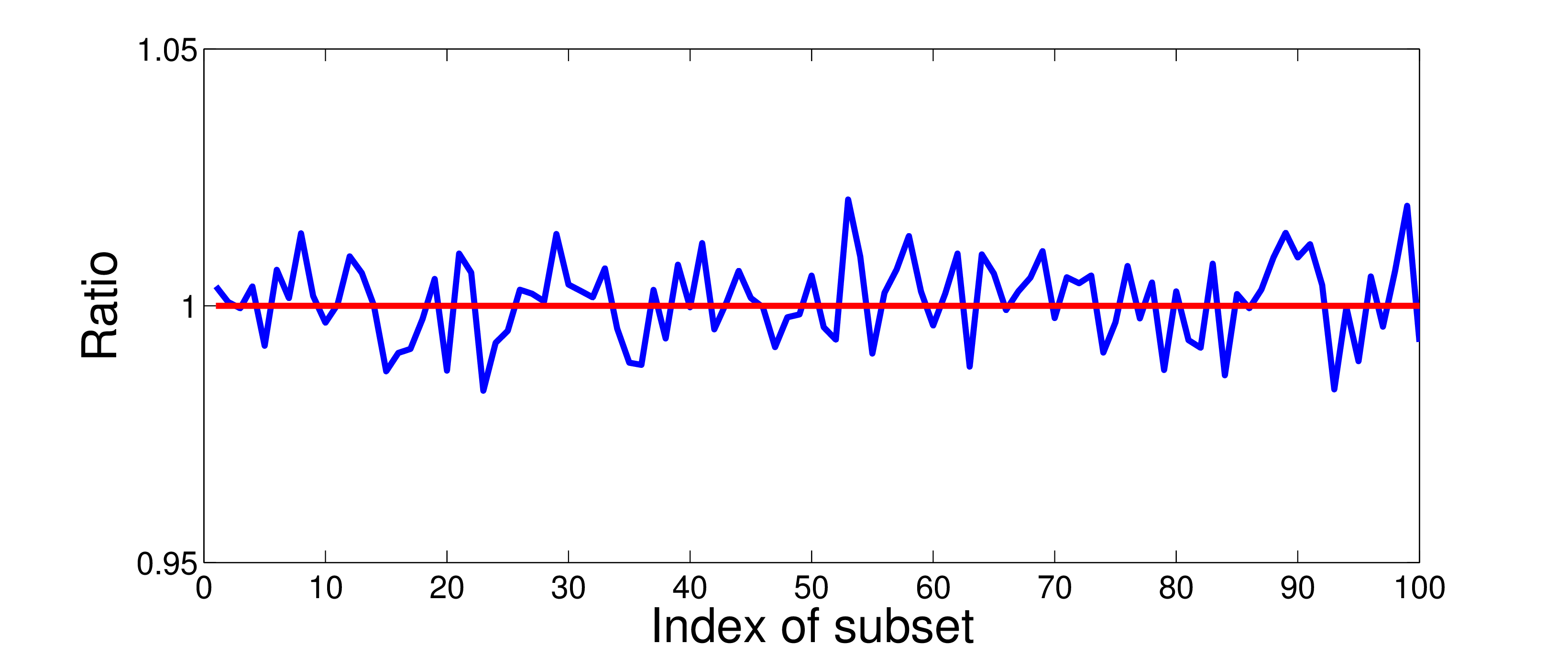
In this work, instead of using the low-rank approximated Gauss-Newton Hessian to construct the proposal distribution as in Martin et al. (2012), we use the l-BFGS Hessian to build the proposal distribution. As a result, we do not require the low-rank assumption and the additional computational cost associated with the low-rank representative of the Gauss-Newton Hessian in each iteration. In order to construct the l-BFGS hessian close enough to the true Hessian, we start the construction from a pseudo Gauss-Newton Hessian (Choi, Min, & Shin, 2008), which is a diagonal matrix with properly scaling. The pseudo Hessian is then continuously updated by the addition of two 1-rank matrices in each iteration. Additionally, during each iteration, we use the randomized source sub-sampling method to reduce the computational cost of evaluating the posterior pdf, gradient and l-BFGS Hessian, and these limit the number of PDE solves. Friedlander & Schmidt (2012) provided an extensive comparison and analysis between the sub-sampling gradient and the full gradient. In our previous work (Fang et al., 2014), we also showed that the randomized source sub-sampling method only introduced a small relative error (Figure 1).

After constructing the local l-BFGS Hessian \(\H_{k}\) and gradient \(\g_{k}\), we define the local Gaussian \[ \begin{equation} \label{LocalGauss} q(\v_{k},\y)\propto \exp\left(-\frac{1}{2}\left(\y-\v_{k}+\H_{k}^{-1}\g_{k}\right)^{T}\H_{k}\left(\y-\v_{k}+\H_{k}^{-1}\g_{k}\right)\right) \end{equation} \] as the proposal distribution. The proposal sample \(\y\) from this distribution can be generated as follows: \[ \begin{equation} \label{GenerateY} \y = \v_{k}-\H_{k}^{-1}\g_{k} + \H_{k}^{-1/2}\gamma, \end{equation} \] where \(\gamma\) is a random vector from the normal distribution \(\mathcal{N}(0,\mathbf{I})\). Finally, we use the M-H criterion to accept or reject the proposal sample \(\y\). The pseudocode for the stochastic quasi-Newton McMC algorithm is given in Algorithm 2.

Numerical experiment

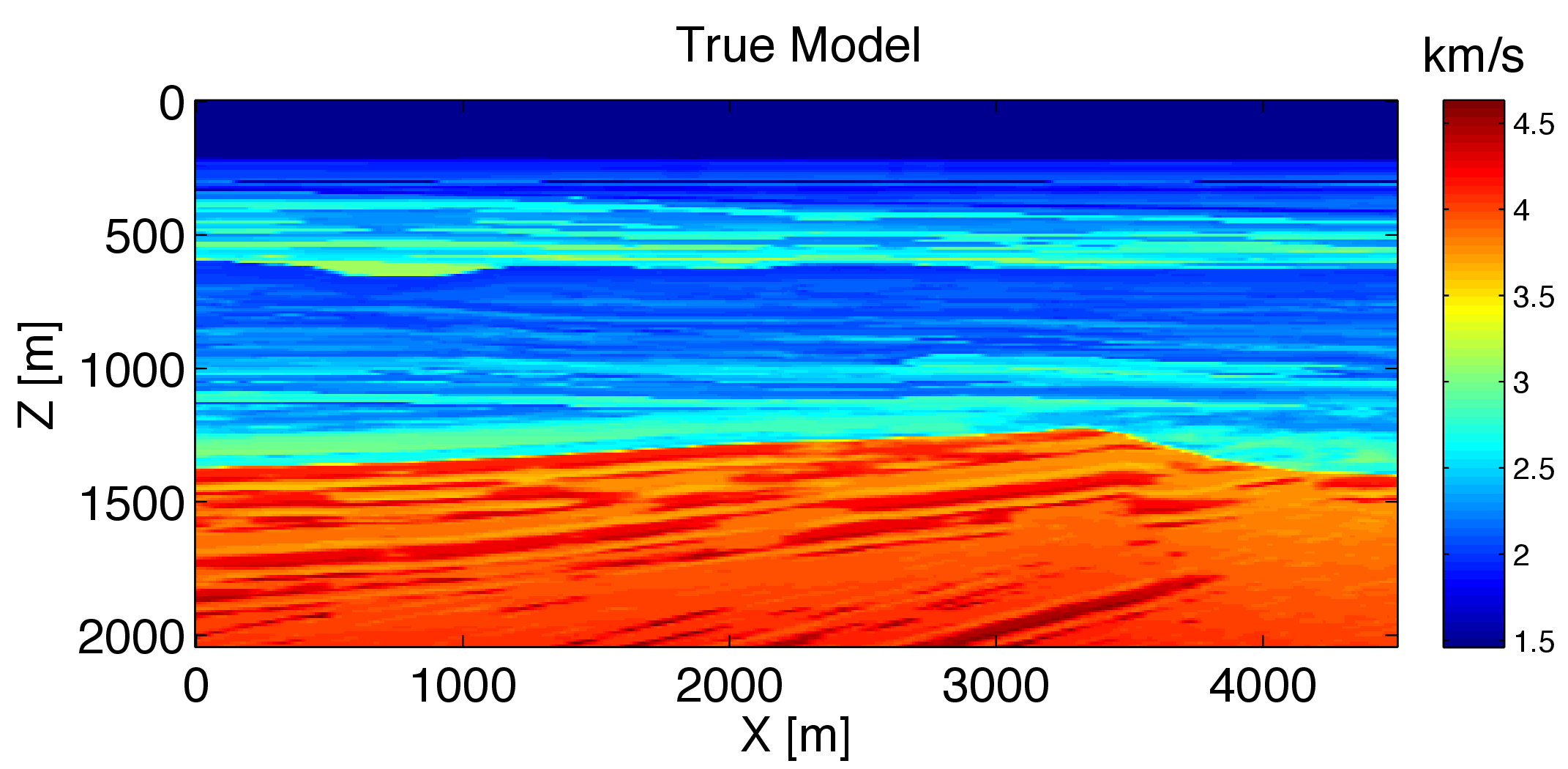
To illustrate the capability of the stochastic quasi-Newton McMC method to quantify the uncertainty of FWI with a considerable small cost, we consider the following experiment on a domain of 2 km by 4.5 km shown in Figure 2a. The synthetic observed data \(\d_{\obs}\) is generated by solving the Helmholtz equation using an optimal 9-points finite difference method (Jo & Suh, 1996) in 15 equally-spaced frequencies ranging from 3 Hz to 17 Hz. Both sources and receivers are located at depth \(z = 20\) m with 50 m and 10 m horizontal sampling interval, respectively. The source wavelet is a Ricker wavelet with central frequency of 12 Hz.

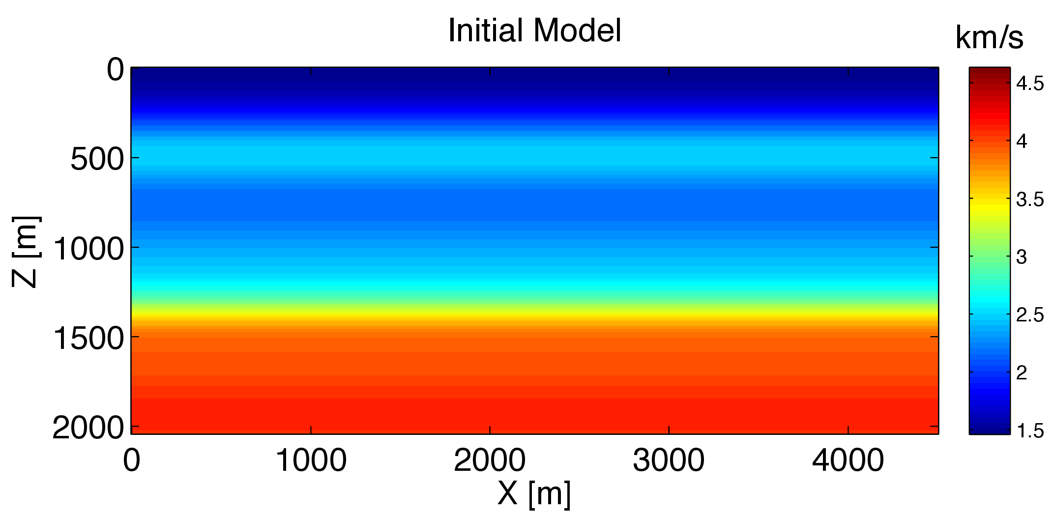
For this numerical experiment, we set the noise covariance matrix to a diagonal matrix whose standard deviation is 0.1. We assume we do not have any special prior information, thus we set the prior model \(\overline{\v}_{\prior}\) to the initial model (c.f. Figure 2b), which is obtained by smoothing the true model followed by a horizontal stack. The prior covariance matrix is set as a diagonal matrix with relative standard deviation of 0.1.

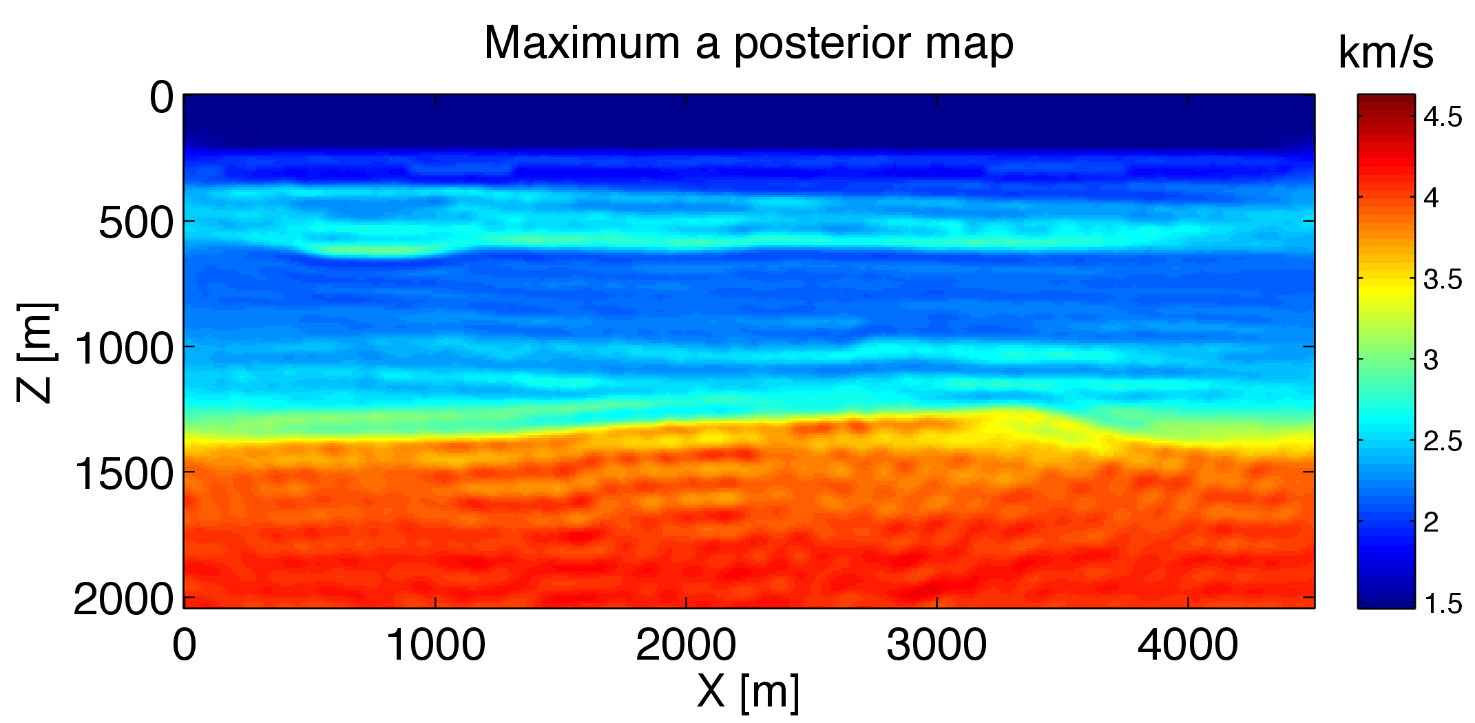
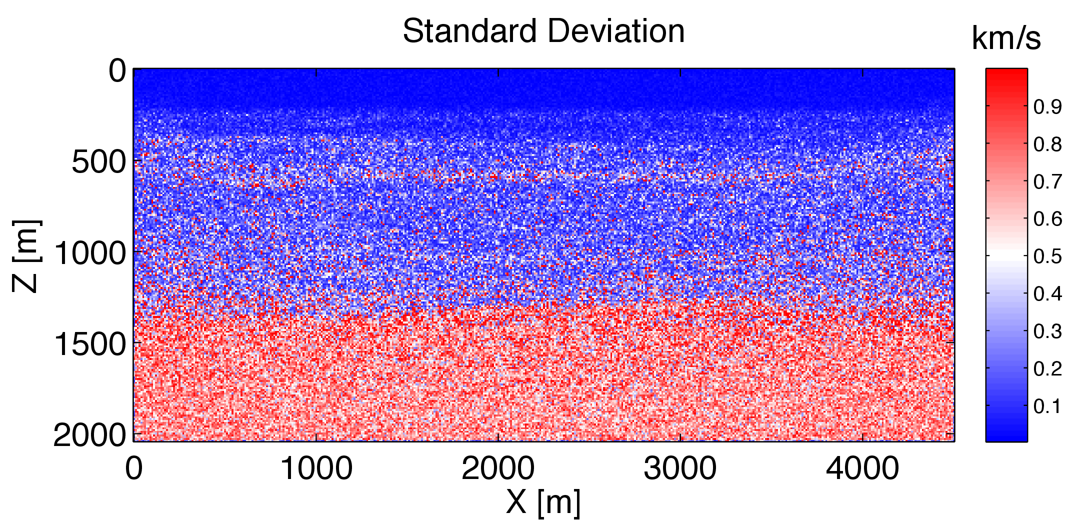
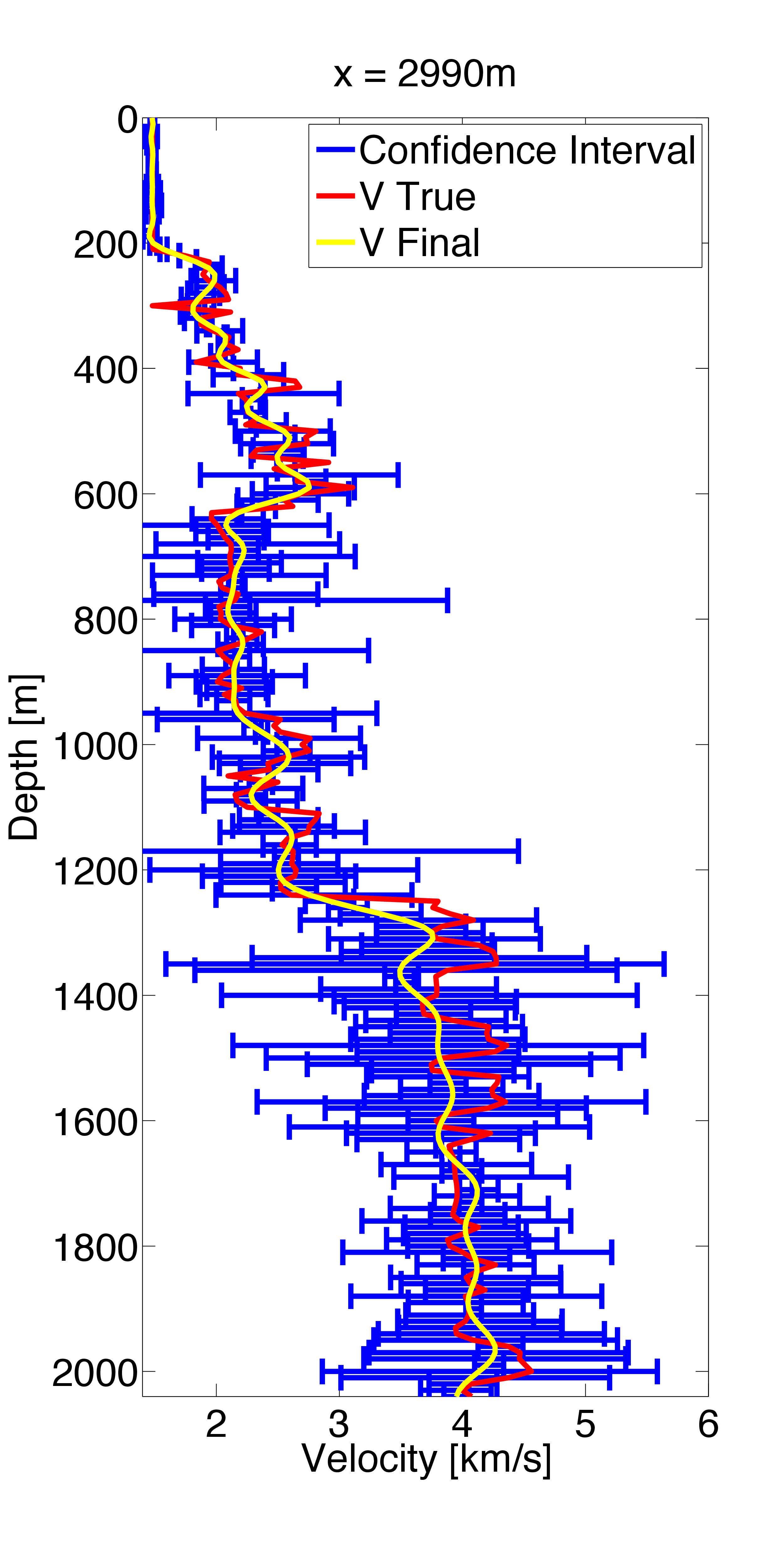
In the uncertainty quantification procedure, we first invert the maximum a posterior (MAP) estimate of the posterior distribution. As a custom strategy of FWI, We invert the MAP estimate in consecutive (five) frequency bands and use the previous result as a warm start for the inversion of the next frequency band. We use the stochastic l-BFGS method (Leeuwen & Herrmann, 2013) to obtain the MAP estimate \(\v_{\text{MAP}}\) plotted in Figure 3a. Then we start from the \(\v_{\text{MAP}}\) and use the stochastic quasi-Newton McMC algorithm (Algorithm 2) to sample the posterior distribution \(\rho_{\post}\). During each iteration, only 5 of all 91 shots are randomly selected to calculate the posterior pdf, gradient and l-BFGS Hessian. We quantify the uncertainties based on these samples and obtain the standard deviation of velocity at each grid (Figure 3b) and the confidence interval (Figure 4) at three different horizontal position (x = 1490 m, 2240 m, and 2990 m).

Discussion

The l-BFGS Hessian is used to construct the proposal distribution, so the computational cost in each iteration only involves the calculation of the posterior pdf and the gradient. Comparing with the random walk Metropolis method, the stochastic quasi-Newton McMC method only requires an additional computational cost for generating the gradient during each iteration, while it is able to construct a much better proposal distribution containing more information about the true posterior distribution to speed up the convergence of the Markov chain. Comparing with the original Newton type McMC method (Martin et al., 2012), although the l-BFGS Hessian may be less accurate, the additional computational cost for estimating the low-rank approximation is eliminated, which results in a significant computational cost reduction. Moreover, without the requirement of the low-rank assumption of the misfit Gauss-Newton Hessian, this method will not suffer from the instability introduced by violating the low-rank assumption. As a result this method may be more suitable for seismic exploration.

Moreover, since the randomized source sub-sampling method is used, in each iteration, only 5 randomly selected sources are used to calculate the approximated posterior pdf and gradient, and thus the computational cost is only 1/18 of that using all sources, effectively speeding up the computation by a factor of 18. In addition, the total computational cost for each iteration is considerably less than that of only evaluating the posterior pdf with all sources, which means the stochastic quasi-Newton McMC is even cheaper than the random walk Metropolis method with all sources.

Due to the computational capability, we only generate 1000 samples and accept 289 samples, which results in the noise in the standard deviation map (Figure 3b). Comparing results of the MAP estimate (Figure 3a) and standard deviation (Figure 3b), we observe that the velocity of deep areas, strong contrast areas and boundaries has larger uncertainties than that of shallow areas, weak contrast areas and central areas, as expected. A similar observation can be drawn for confidence interval (Figure 4). Here the probability is more concentrated at shallow areas and low velocity contrast areas than deep areas and strong velocity contrast areas.

Finally, the artifacts associated with the poor prior model still can be observed in the MAP estimate, which implies us the importance of selecting a good prior model. For the situation that no special prior information exists in advance, one alternative solution may be to update the prior model after the inversion of each frequency band.

Conclusion

In this work, we formulate the uncertainty quantification problem of FWI in the Bayesian inference framework, and propose a stochastic quasi-Newton McMC method to solve this problem. Using the l-BFGS Hessian as the inverse of the covariance matrix, we release the low-rank assumption and reduce the computational cost for constructing the proposal distribution of the Metropolis-Hasting method. Additionally, we use the randomized source sub-sampling strategy to speed up the evaluation of the posterior pdf, gradient and Hessian. As a result, we obtain a fast McMC method to quantify the uncertainty of FWI. While initial results are encouraging, several challenges remain such as the credence of the l-BFGS as a good approximation of the true Hessian.

Acknowledgements

This work was financially supported in part by the Natural Sciences and Engineering Research Council of Canada Discovery Grant (RGPIN 261641-06) and the Collaborative Research and Development Grant DNOISE II (CDRP J 375142-08). This research was carried out as part of the SINBAD II project with support from the following organizations: BG Group, BGP, BP, Chevron, ConocoPhillips, CGG, ION GXT, Petrobras, PGS, Statoil, Total SA, WesternGeco, Woodside. We also thank BG Group for providing the synthetic model we used in our example.

References

Bui-Thanh, T., Ghattas, O., Martin, J., & Stadler, G. (2013). A Computational Framework for Infinite-Dimensional Bayesian Inverse Problems Part I: The Linearized Case, with Application to Global Seismic Inversion. SIAM Journal on Scientific Computing, 35(6), A2494–A2523. Retrieved from http://epubs.siam.org/doi/abs/10.1137/12089586X
Choi, Y., Min, D.-J., & Shin, C. (2008). Frequency-domain Elastic Full Waveform Inversion Using the New Pseudo-Hessian Matrix: Experience of Elastic Marmousi-2 Synthetic Data. Bulletin of the Seismological Society of America, 98(5), 2402–2415. doi:10.1785/0120070179
Fang, Z., Silva, C. D., & Herrmann, F. J. (2014, January). Fast Uncertainty Quantification for 2D Full-waveform Inversion with Randomized Source Subsampling. 76th eAGE. Retrieved from https://www.slim.eos.ubc.ca/Publications/Public/Conferences/EAGE/2014/fang2014EAGEfuq.pdf
Friedlander, M., & Schmidt, M. (2012). Hybrid Deterministic-Stochastic Methods for Data Fitting. SIAM Journal on Scientific Computing, 34(3), A1380–A1405. Retrieved from http://epubs.siam.org/doi/abs/10.1137/110830629
Jo, S., C., & Suh, J. (1996). An Optimal 9-Point, Finite-Difference, Frequency-Space, 2-d Scalar Wave Extrapolator. GEOPHYSICS, 61(2), 529–537. doi:10.1190/1.1443979
Kaipio, J., & Somersalo, E. (2004). Statistical and Computational Inverse Problems (Applied Mathematical Sciences) (v. 160) (1st ed.). Hardcover; Springer. Retrieved from http://www.amazon.com/exec/obidos/redirect?tag=citeulike07-20\&path=ASIN/0387220739
Leeuwen, T. van, & Herrmann, F. J. (2013). Fast Waveform Inversion without Source-Encoding. Geophysical Prospecting, 61, 10–19. Retrieved from http://dx.doi.org/10.1111/j.1365-2478.2012.01096.x
Martin, J., Wilcox, L., Burstedde, C., & Ghattas, O. (2012). A Stochastic Newton MCMC Method for Large-scale Statistical Inverse Problems with Application to Seismic Inversion. SIAM Journal on Scientific Computing, 34(3), A1460–A1487. Retrieved from http://epubs.siam.org/doi/abs/10.1137/110845598
Virieux, J., & Operto, S. (2009). An Overview of Full-waveform Inversion in Exploration Geophysics. GEOPHYSICS, 74(6), WCC1–WCC26. Retrieved from http://library.seg.org/doi/abs/10.1190/1.3238367