Wave simulation

Background

Since its re-introduction by Pratt (1999), Full-Waveform Inversion (FWI) has gained major attention by the computational seismology community because of its ability to build high-resolution velocity models more or less automatically in areas of complex geology. Because FWI relies on numerical solutions of the wave-equation, FWI calls for fast and scalable wave-equation solvers that can handle non-trivial representations of the physics.

At SLIM, we have always focused on the development of high-level abstractions to facilitate rapid research and development in computational seismology and other related fields such as [Medical imaging]. This call for scalable abstracted parallel implementations for the wave physics has resulted in the inception of Devito, a Domain-Specific Language (DSL) for finite-difference calculations and more generally stencil computation (F. Luporini et al., 2020; M. Louboutin et al., 2019). To gain easy access to Devito’s highly optimized wave-propagators needed to solve industry-scale wave-equation based inverse problems (RTM, SPLS-RTM, and FWI), we built the Julia Devito Inversion Framework JUDI (P. A. Witte et al., 2019), for traditional high-performance systems, and JUDI4Cloud for Cloud Computing. Because this framework makes use of linear algebra abstractions, it seamlessly integrated with JOLI - Julia Operators LIbrary and our (convex) Optimization packages SlimOptim and SetIntersectionProjection.

Below, we briefly introduce seismic modeling with Devito’s DSL. With this introduction, we lay the groundwork for wave-equation based inversion using JUDI. For details on the actual application of scalable Devito-based inversions, we refer to Imaging, Full-Waveform Inversion, and Monitoring.

Wave simulations for inversion with Devito

As mentioned before, Devito provides a concise and straightforward computational framework for discretizing wave-equations, which form an essential component of wave-based inversions including RTM and FWI. By means of code snippets, we will show that Devito generates verifiable executable C code at run time for wave propagators associated with forward and adjoint wave-equations¹. Through the use of math-inspired abstractions, Devito frees the user from the recurrent and time-consuming development of high-performance time-stepping finite-difference codes and allows the user to concentrate on the geophysics of the problem rather than on low-level implementation details of wave-equation simulators. This brief tutorial covers the conventional adjoint-state formulation of full-waveform tomography (Tarantola, 1984) that undergirds wave-equation based inversion (Virieux and Operto, 2009). While SLIM has been responsible for the derivation of alterative formulations for FWI, these will be discussed under Wavefield Reconstruction Inversion. Here, we will concentrate on the standard formulation that relies on the combination of a forward/adjoint pair of propagators and a correlation-based gradient. First, we discuss how to set up [Wave simulations for inversion], including how to express the wave-equation symbolically in Devito and how to deal with the acquisition geometry.

Tutorial for wave simulations with Devito

The acoustic wave equation

The acoustic wave-equation with the squared slowness \(m\), defined as \(m(x,y)=c^{-2}(x,y)\) with \(c(x,y)\) being the unknown spatially varying compressional wavespeed, is given by \[ \begin{equation} m(x, y) \frac{\mathrm{d}^2 u(t, x, y)}{\mathrm{d}t^2}\ -\ \Delta u(t, x, y)\ +\ \eta(x, y) \frac{\mathrm{d} u(t, x, y)}{\mathrm{d}t}\ \ =\ \ q(t, x, y; x_\mathrm{s}, y_\mathrm{s}), \label{wave} \end{equation} \] where the symbol, \(\Delta\), stands for the Laplace operator, \(q(t, x, y;x_\mathrm{s}, y_\mathrm{s})\) denotes the seismic source signature, located at \((x_\mathrm{s}, y_\mathrm{s})\), and \(\eta(x, y)\) is a space-dependent dampening parameter for the absorbing boundary layer (Cerjan et al., 1985). As shown in Figure 2, the physical model is extended in every direction by nbpml grid points to mimic an infinite domain. The damping term \(\eta\, \mathrm{d}u/\mathrm{d}t\) attenuates the waves in the absorbing boundary layer, which prevents waves from reflecting at the edges of the model. In Devito, the discrete representations for \(m\) and \(\eta\) are contained in a model object that contains a grid object with all relevant information, such as the origin of the coordinate system, grid spacing, size of the model and dimensions time, x, y:

# Define a velocity model. The velocity is in km/s
N = (401, 401)
model = demo_model('layers-isotropic',  # A velocity model.
                   nlayers=6, # Number of layers
                   shape=N, # Number of grid points.
                   spacing=(7.5, 7.5),  # Grid spacing in m.
                   nbl=80, space_order=8)  # boundary layer.
vp = model.vp.data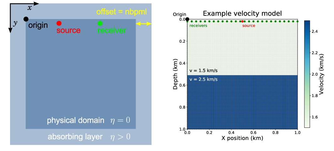

After executing this code, running

# Quick plot of model.
plot_velocity(model)

creates the velocity model depicted in Figure 3.

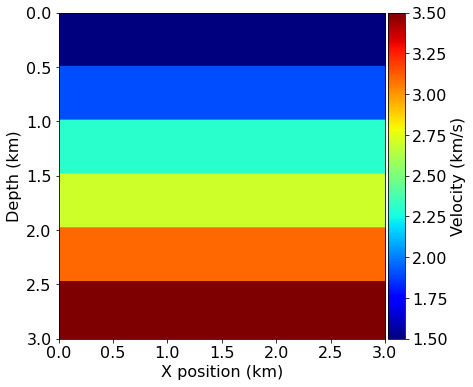
In this Model instantiation, vp is the velocity in \(\text{km}/\text{s}\), origin is the origin of the physical model in meters, spacing is the discrete grid spacing in meters, shape is the number of grid points in each dimension and nbpml is the number of grid points in the absorbing boundary layer. It is important to note that shape is the size of the physical domain only, while the total number of grid points, including the absorbing boundary layer, will be automatically derived from shape and nbpml.

Symbolic definition of wave propagators

To model seismic data by solving the acoustic wave-equation, the first necessary step is to discretize this partial differential equation (PDE), which includes discrete representations of the velocity model, the wavefields, and the sources/receivers, as well as approximations of the spatial and temporal derivatives using finite-differences (FD). Unfortunately, implementing these finite-difference schemes in low-level code by hand is error-prone, especially when reliable high-performance 3D code is needed.

For this reason, the primary design objective of Devito is to allow users to define complex matrix-free finite-difference approximations from high-level symbolic definitions for the wave-equation, while employing automated code generation to create highly optimized low-level C code. Through the use of the symbolic algebra package SymPy (Meurer et al., 2017), Devito automatically creates expressions for the derivatives from which Devito generates computationally efficient wave propagators.

At the core of Devito’s symbolic API are symbolic types that behave like SymPy function objects, while also managing data

• Function objects represent a spatially varying function discretized on a regular Cartesian grid. For example, the function symbol f = Function(name='f', grid=model.grid, space_order=2) is denoted symbolically as f(x, y). These objects provide auto-generated symbolic expressions for finite-difference derivative operators through shorthand expressions like f.dx and f.dx2 for the first and second derivative along the x-coordinate.

• TimeFunction objects represent time-dependent functions that have \(\text{time}\) as the leading dimension, for example g(time, x, y). In addition to spatial derivatives TimeFunction symbols also provide time derivatives g.dt and g.dt2.

• SparseFunction objects represent sparse components, such as sources and receivers, which are usually distributed sparsely and often located off the computational grid. These objects handle interpolation onto the model grid.

To demonstrate Devito’s symbolic basic capabilities, let us consider the Python code for a time-dependent function \(\mathbf{u}(\text{time}, x, y)\) representing the discrete forward wavefield

t0 = 0.     # Simulation starts a t=0
tn = 3000.  # Simulation last 1 second (1000 ms)
dt = model.critical_dt  # Time step from model grid spacing

nt = int(1 + (tn-t0) / dt)  # Discrete time axis length
time = TimeAxis(start=t0, stop=tn, step=dt)  # Discrete modelling time
u = TimeFunction(name="u", grid=model.grid, 
                 time_order=2, space_order=8,
                 save=time.num)

where the grid object provided by the model defines the size of the allocated memory region. The time_order and space_order define the default discretization order of the finite-difference approximations for the derivative expressions.

Using shorthand expressions, such as u.dt and u.dt2 to denote \(\frac{\text{d} u}{\text{d} t}\) and \(\frac{\text{d}^2 u}{\text{d} t^2}\), we can now write a symbolic representation for the wave-equation that needs to be solved to generate our wavefields. Our solution based on time stepping is derived from discretized expressions for the finite-difference derivative approximations generated by Devito. Given these symbolic expressions, the source-free version of Equation \(\ref{wave}\) can be written as

pde = model.m * u.dt2 - u.laplace + model.damp * u.dt

In this expression, we made use of the model object, which we created earlier, and which already contains the squared slowness \(\mathbf{m}\) and damping term \(\mathbf{\eta}\) as Function objects.

If we write out the (second order) second time derivative u.dt2 and ignore the damping term for the moment, our pde expression translates into the following discrete the wave-equation: \[ \begin{equation} \frac{\mathbf{m}}{\text{dt}^2} \Big( \mathbf{u}[\text{time}-\text{dt}] - 2\mathbf{u}[\text{time}] + \mathbf{u}[\text{time}+\text{dt}]\Big) - \Delta \mathbf{u}[\text{time}] = 0, \quad \text{time}=1 \cdots n_{t-1} \label{pde1} \end{equation} \] with \(\text{time}\) being the current time step and \(\text{dt}\) being the time stepping interval. To propagate the wavefield, we rearrange the terms in this equation to obtain an expression for the wavefield \(\mathbf{u}(\text{time}+\text{dt})\) at the next time step from the wavefield at the previous timestep. Ignoring the damping term once again, this yields \[ \begin{equation} \mathbf{u}[\text{time}+\text{dt}] = 2\mathbf{u}[\text{time}] - \mathbf{u}[\text{time}-\text{dt}] + \frac{\text{dt}^2}{\mathbf{m}} \Delta \mathbf{u}[\text{time}]. \label{pde2} \end{equation} \] By using the Devito utility function solve, this rearrangement of terms can be done automatically, creating an expression that defines the wavefield updates for the next timestep \(\mathbf{u}(\text{time}+\text{dt})\), with the command u.forward:

stencil = Eq(u.forward, solve(pde, u.forward))

The stencil object represents the finite-difference approximation derived from Equation \(\ref{pde2}\), including the finite-difference approximation of the Laplacian and the damping term. Although it defines the update for a single timestep only, Devito knows that we will be solving a time-dependent problem over large numbers of timesteps because the wavefield u is a TimeFunction object. In Advanced simulations, we will include more elaborate examples. For further details, we refer to Devito documentation and JUDI documentation.

Setting up the acquisition geometry

So far, the expression and code for the time stepping derived in Symbolic definition of wave propagators do not contain a source term. While this suffices when dealing with initial state problems, active-source seismic experiments are often excited by impulsive sources, \(q(x,y,t;x_\text{s})\), which are functions of space and time (just like the wavefield u). To include an impulsive source term in our modeling scheme, we simply add the source wavefield as an additional term to Equation \(\ref{pde2}\) — i.e., we have \[ \begin{equation} \mathbf{u}[\text{time}+\text{dt}] = 2\mathbf{u}[\text{time}] - \mathbf{u}[\text{time}-\text{dt}] + \frac{\text{dt}^2}{\mathbf{m}} \Big(\Delta \mathbf{u}[\text{time}] + \mathbf{q}[\text{time}]\Big). \label{eqsrc} \end{equation} \] Since the source appears on the right-hand side of the original equation (Equation \(\ref{wave}\)), that term also needs to be multiplied with \(\frac{\text{dt}^2}{\mathbf{m}}\) (this follows from rearranging Equation \(\ref{pde1}\), with the source on the right-hand side instead of the 0). Unlike the discrete wavefield u, however, the source q is typically localized in space and only a function of time, which means the time-dependent source wavelet is injected into the propagating wavefield at a specified source location. The same applies when the wavefield is sampled at the receiver locations when simulating shot records. In practice, source and receiver locations do not necessarily coincide with the modeling grid. In code, we have

f0 = 0.020  # kHz, peak frequency.
src = RickerSource(name='src', grid=model.grid, f0=f0,
                   time=time, coordinates=src_coords)

where RickerSource acts as a wrapper around SparseFunction and models a Ricker wavelet with a peak frequency f0 and source coordinates src_coords. The src.inject function below injects at the specified coordinates the current time sample of the Ricker wavelet (weighted with \(\frac{\text{dt}^2}{\mathbf{m}}\) as shown in Equation \(\ref{eqsrc}\)) into the updated wavefield u.forward via

src_term = src.inject(field=u.forward, expr=src * dt**2 / model.m)

To extract the wavefield at a predetermined set of receiver locations, there is a corresponding wrapper function for the receivers, which creates a SparseFunction object for a given number npoint of receivers, number nt of time samples, and specified receiver coordinates rec_coords:

rec = Receiver(name='rec', npoint=101, ntime=nt,
               grid=model.grid, coordinates=rec_coords)

Rather than injecting a function into the model as we did for the source, we now simply save the wavefield at the grid points that correspond to receiver positions and interpolate the data to their exact position of the computational grid location:

rec_term = rec.interpolate(u)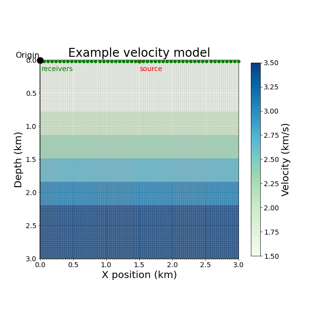

With the acquisition geometry defined and plotted in Figure 4, we can now derive code for our propagators.

Forward simulation

By adding the source and receiver terms to our stencil object, we can now define our forward propagator

op_fwd = Operator([stencil] + src_term + rec_term)

The symbolic expressions used to create Operator contain sufficient meta-information for Devito to create a fully functional computational kernel. The dimension symbols contained in the symbolic function object (time, x, y) define the loop structure of the created code, while allowing Devito to automatically optimize the underlying loop structure to increase execution speed.

At run-time, the size of the loops and spacing between grid points are inferred from the symbolic Function objects and associated model.grid object. By supplying the timestep size dt, we can invoke the generated kernel through a simple Python function call. The user data associated with each Function is updated in-place during operator execution, allowing us to extract the final wavefield and shot record directly from the symbolic function objects without unwanted memory duplication via

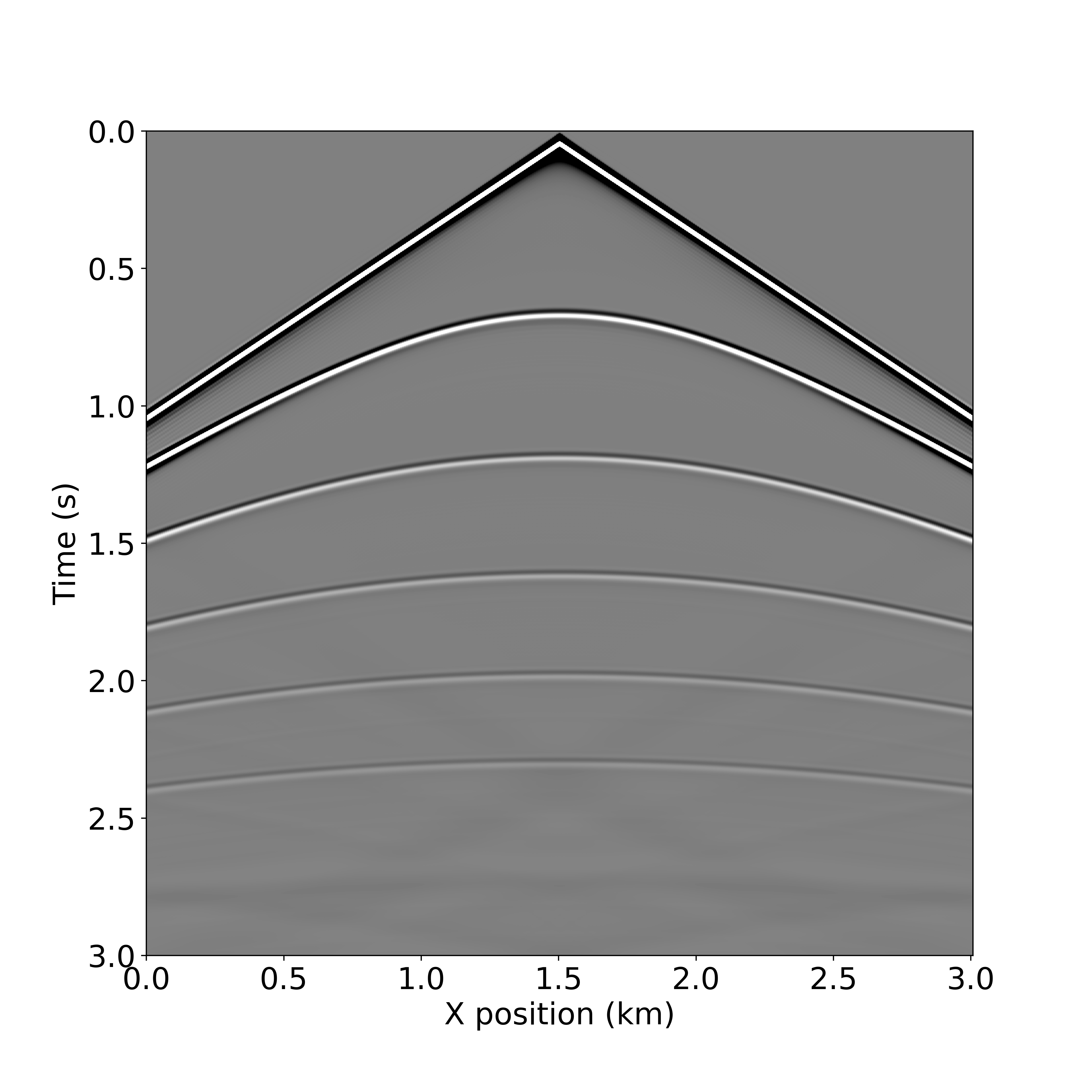
op_fwd(dt=model.critical_dt)

When this code has finished running, the resulting wavefield is stored in u.data and the shot record is in rec.data. As shown in Figure 5, this 2D array can easily be plotted as an image.

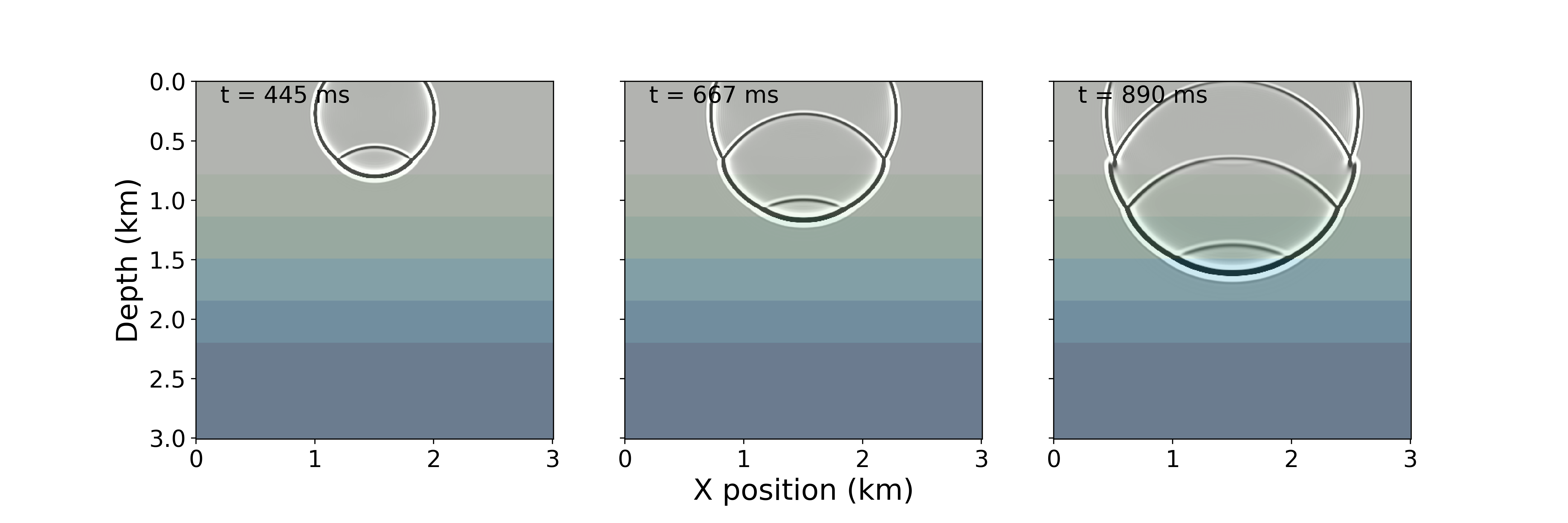
As demonstrated in the notebook, a movie of snapshots of the forward wavefield can also be generated by capturing the wavefield at discrete timesteps. Figure 6 shows three timesteps from the movie below.

Advanced simulations

Thanks to this abstraction, we can easily develop wave propagators better suited to represent the Earth’s subsurface. While the acoustic isotropic wave-equation is widely used to develop algorithms and inversion frameworks for its simplicity, real-world data requires more representative equations. We present here a few advanced modeling examples highlighting the capabilities and scalability of SLIM software.

Forward and adjoint TTI simulations

The first equation we consider is the most commonly used equation for field data, the transverse tilted isotropic (TTI) wave-equation. This equation models the anisotropic behavior of the subsurface in an acoustic approximation allowing for an accurate wavefield while avoiding the computational and memory burden of full elastic propagators. One of the main complexity of the TTI wave-equation is that, unlike the isotropic acoustic equation, the PDE system is not self-adjoint dues to the approximations made to derive its expressions. We have shown in the past that the use of the proper adjoint for this equation is mandatory for accurate imaging of the subsurface (Louboutin et al., 2018). Consequently, our modeling and inversion propagators (in JUDI) implement the TTI wave-equation and its true adjoint to allow for real-world applications. We show a snapshot of the TTI forward and adjoint wavefield in the BP 2007 TTI model for illustration on Figure #ttiwf.

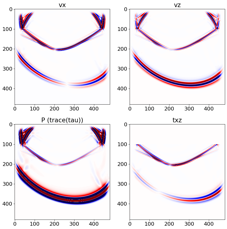
Elastic simulations

As a proof of concept to demonstrate the simplicity and the ease of development with Devito, we have implemented a 2D TTI elastic propagator using rotated staggered-grid finite-difference for higher accuracy (Gao and Huang, 2017). The implementation is available at Elastic TTI. With the high-level definition of an elastic stiffness tensor, Devito then allows to define the TTI elastic wave-equation in a three-line succinct mathematical way as one would write it on paper:

# Equation
C = SeismicStiffness(grid.dim, vp, vs=vs, rho=rho, epsilon=epsilon, delta=delta, theta=theta)
u_v = Eq(v.forward, damp*(v + dt/rho*divrot(tau)))
e = 1 / 2 * (gradrot(v.forward) + gradrot(v.forward).T)
u_t = Eq(tau.forward, damp*(tau + dt * C.prod(e)))

We show for illustration a snapshot of the particle velocities and stresses on Figure 9.

Ongoing research

With Devito we can now easily define and model complex physics representations such as the TTI or elastic wave-equations. One of the main complexity arising from these advanced representations is the extended computational and memory cost of inversion. The core research direction in seismic modeling relies on machine learning to design discretizations that allow to work on much coarser grid while conserving high accuracy. This work is inspired by recent advances in the field of computational Fluid Dynamics (Bar-Sinai et al., 2019) where the simpler case of diffusive or Elliptique equation can be solved on coarser grid using learned discretizations.

For wave-equation bases inversions, see Imaging and Full-waveform inversion.

References

Supplemental material

• Devito documentation
• Devito source code and examples
• Tutorial notebooks
• JUDI homepage