A dual formulation of wavefield reconstruction inversion for large-scale seismic inversion

Abstract

Most of the seismic inversion techniques currently proposed focus on robustness with respect to the background model choice or inaccurate physical modeling assumptions, but are not apt to large-scale 3D applications. On the other hand, methods that are computationally feasible for industrial problems, such as full waveform inversion, are notoriously bogged down by local minima and require adequate starting models. We propose a novel solution that is both scalable and less sensitive to starting model or inaccurate physics when compared to full waveform inversion. The method is based on a dual (Lagrangian) reformulation of the classical wavefield reconstruction inversion, whose robustness with respect to local minima is well documented in the literature. However, it is not suited to 3D, as it leverages expensive frequency-domain solvers for the wave equation. The proposed reformulation allows the deployment of state-of-the-art time-domain finite-difference methods, and is computationally mature for industrial scale problems.

Introduction

Field-data applications of wave-equation based seismic inversion are limited by the computational complexity of large-scale 3D simulations, and by the tendency of traditional inversion techniques (such as full waveform inversion, FWI, Tarantola and Valette, 1982) to converge to unrealistic models. While considerable advances have been made to speed up wave equation solvers and avoid local minima, most of the currently proposed inversion methods do not take advantage of both these developments, and are practically limited to 2D problems. In this paper, we introduce a novel method that is fit for 3D large-scale deployment and relatively robust against spurious minima.

We adopt model extension methods that aim at counteracting local minimum stagnation, which are based on a reformulation of the original inverse problem into a higher dimensional space of unknowns (Symes, 2008). While beneficial for avoiding local minima, the inherent added complexity of these methods typically curtails large-scale applications. One notable example, and the basis for this work, is wavefield reconstruction inversion (WRI, van Leeuwen and Herrmann, 2013), which has demonstrated robustness towards local minima but is not well suited for 3D problems. Indeed, WRI involves the solution of an extended wave equation that is conventionally solved in the frequency domain with direct or iterative methods, although not efficiently for large grid sizes. Many other methods related to WRI share, fundamentally, the same limitation (Huang et al., 2017, 2018; Aghamiry et al., 2019).

We propose a principled Lagrangian reformulation of classical WRI, referred to as WRI\(\ast\) throughout the text, which naturally lends itself to time-domain solvers, hence large-scale applications. The reformulation is based on minimizing the wave equation error and interpreting the data misfit as a constraint. Complexity analysis and numerical experimentation highlights comparable computational costs to FWI per gradient computation (corresponding to roughly twice its cost), and is consistently more robust with respect to starting model and inexact physical modeling assumptions. Contrary to most of the inversion methods based on the wave equation nowadays available, our approach represents a computationally efficient, robust, and ultimately feasible proposal for 3D seismic inversion.

Our proposal leverages on the current state-of-the-art in time-domain finite-difference solvers that ensures scalability on the hardware available to the oil-and-gas industry, or even to a wider audience thanks to cloud computing (Witte et al., 2020). We employ the domain-specific language Devito for automatic generation of highly optimized finite-difference C code (Luporini et al., 2020; Luporini et al., 2018; Louboutin et al., 2019). Here, we focus on acoustic modeling and pseudo-acoustic modeling with tilted transverse isotropy (TTI, Alkhalifah, 2000), established as a reasonable compromise between realistic physics and computational feasibility.

The computational and theoretical advantages of WRI\(\ast\) will be demonstrated with extensive 2D experimentation. Despite the central claim of the paper being centered on 3D feasibility, 3D problems are still beyond the economic resources realistically available to academic organizations, and will not be included in this work. We stress, however, that this is not due to a fundamental limitation of the method, and any institution that can afford the computations needed for FWI can also fruitfully employ WRI\(\ast\).

In the rest of this paper, we discuss the computational and theoretical pitfalls of classical seismic inversion, with a general overview of the methods that deal with those issues. We review Lagrangian and reduced formulations for seismic inversion, followed by a more in-depth discussion on WRI. The main section is devoted to the reformulation of WRI object of this work: WRI\(\ast\). Lastly, we present numerical experiments to thoroughly test our proposal and compare it to conventional WRI and FWI.

Seismic inversion: computational and theoretical complexity

Modern seismic inversion, such as FWI, is cast as an optimization problem endowed with partial differential equation constraints (Virieux and Operto, 2009). Given a suitable discretization of the physical quantities of interest, and the algebraic operators that govern their mutual relationship, the problem can be succinctly expressed as: \[ \begin{equation} \min_{\bmm,\bu}\dfrac{1}{2}\norm{\bd-\R\bu}^2\quad\mathrm{subject\ to}\quad\A\bu=\bq. \label{eq:invprobgen} \end{equation} \] Data \(\bd\in\Real^{\Nr\times\Nt\times\Ns}\) are recorded in time at \(\Nr\) receiver locations for different \(\Ns\) source positions. Alternatively, after a temporal Fourier transform, \(\bd\in\Compl^{\Nr\times\Nf\times\Ns}\) for \(\Nf\) frequencies. The variable \(\bu\in\Real^{N\times\Nt\times\Ns}\) (or \(\bu\in\Compl^{N\times\Nf\times\Ns}\), in frequency domain) represents a wavefield—e.g. the solution of the wave equation \(\A\bu=\bq\)— discretized on an \(N\)-dimensional space. The right-hand side \(\bq\) of the wave equation is typically a point source. In equation \(\eqref{eq:invprobgen}\), the data are compared to the values of \(\bu\) interpolated at the receiver locations via the operator \(R\), and the misfit calculated via the least-squares norm \(\norm{\cdot}\defeq\norm{\cdot}_2\). The wave operator \(\A\) is parameterized by \(\bmm\), which encapsulates the model unknowns of the problem (e.g. squared slowness, in the simplest acoustic, constant density setting).

In 3D, the grid size grows as \(N=O(n^3)\) (in big \(O\) notation), with \(n\approx1000\) grid points in each direction for a typical industrial-scale problem. With a very conservative source/receiver acquisition coverage, \(\Nr=O(n)\) and \(\Ns=O(n)\). Furthermore, when time-domain methods with explicit time-marching schemes are applied, \(\Nt=O(n)\) (realistically, \(\Nt\approx10\,n\)), due to stability conditions. In the frequency domain, we also often keep \(\Nf=O(n)\), albeit with much more favorable complexity constants than time domain (note that, with optimal frequency sampling, we theoretically only need \(\Nf=O(\log n)\), Sirgue and Pratt, 2004). In this regime, the computational requirements are extremely challenging. For instance, wavefield storage grows as \(O(n^5)\), and cannot be attained for each source/time sample at once. Time complexity is largely dominated by the computation of the solutions of the wave equation. Currently, explicit time-domain methods are favored, as in the frequency domain the wave equation is represented by a large, sparse, non-definite linear system, and neither direct nor iterative methods scale as efficiently to 3D. Frequency domain becomes a palatable option only when a large high-performance computing system can store the matrix factorization (S. Wang et al., 2011), or abundant compute cores are available (Knibbe et al., 2016).

Despite these computational challenges, FWI is now viable for 3D problems of practical size, especially when the simulated physics is restricted to acoustics or tilted transversely isotropic (TTI) pseudo-acoustics (Alkhalifah, 2000; Grechka et al., 2004; Duveneck et al., 2008). The FWI objective functional is, however, highly multimodal and requires considerable problem-specific intervention to be consistently successful when gradient-based optimization is employed. In practice, FWI requires a kinematically correct starting guess to avoid cycle skipping. Local minima have been the subject of a great deal of research in the last 10 years, and many proposals tackling the problem have been advanced. The main lines of investigation involved:

• regularization techniques that penalize unrealistic models, e.g. via total-variation minimization (Esser et al., 2018) or projection onto constraint sets (B. Peters and Herrmann, 2017; B. Peters et al., 2018);
• analysis of data misfit in a transformed domain (Shin and Cha, 2008, 2009; Bozdag et al., 2011) and/or application of preprocessing hierarchical strategies, where different levels of data preconditioning are setup and the associated problems solved sequentially, e.g. low- to high-frequency data filtering inversion (Bunks et al., 1995), or shallow- to deep-model inversion (Shipp and Singh, 2002);
• model extension, where the original problem is generalized to a higher dimensional space better suited for gradient-based optimization (Symes, 2008; van den Berg and Kleinman, 1997; Biondi and Almomin, 2014; van Leeuwen and Herrmann, 2013; C. Wang et al., 2016; R. Wang and Herrmann, 2017a; Aghamiry et al., 2019; Warner and Guasch, 2016; Guasch et al., 2019);
• special objective functionals more amenable to local-search optimization, such as the optimal transport data misfit via the Wasserstein distance (Métivier et al., 2016; Yang et al., 2018; B. Sun and Alkhalifah, 2019).

Note that these approaches are not mutually exclusive, and despite the fact that our contribution is an instance of model extension techniques, preprocessing hierarchical strategies, data transforms, or regularization methods can be incorporated straightforwardly. More recent ideas based on optimal transport can also be formally integrated in the framework presented later on, but requires further study and will not be considered here. Also, the Wasserstein distance needs a careful reinterpretation of seismic data as probability distributions and current solutions are confined to a trace-by-trace comparison, limiting its benefits.

Recently, many model extension methods have been proven successful in their empirical robustness to local minima, but are hampered by the computational costs associated to operating in higher dimension. A notable exception is adaptive waveform inversion (AWI, Warner and Guasch, 2016; Guasch et al., 2019), which consists in matching synthetic time traces to data by means of convolutional Wiener filters with arbitrary length. Since the computational overhead with respect to FWI is affordable, AWI can be applied to large problems. In this paper, however, we are not interested in establishing the relative merits of AWI with respect to other methods, and we will focus on developing a competing method based on WRI. WRI, in its basic formulation (van Leeuwen and Herrmann, 2013), is not amenable to 3D. Indeed, it involves a relaxed version of the wave equation that does not allow for a straightforward implementation of time-marching schemes and is practically limited to 2D problems (see, however, Bas Peters and Herrmann, 2019 for some advances using frequency-domain 3D solvers). Alternative characterizations of the original WRI formulation, as offered in Huang et al. (2017), Huang et al. (2018), or Aghamiry et al. (2019), suffer from the same issues and do not scale efficiently to 3D. The main goal of this paper is to provide a reformulation of WRI that circumvents this limitation.

Reduced, full-space, and penalty formulations

In this section, we lay out the groundwork for WRI and our proposal WRI\(\ast\) by illustrating different ways to deal with the problem formulated in equation \(\eqref{eq:invprobgen}\). Classical FWI consists of imposing the constraint \(\bu=\A^{-1}\bq\) explicitly (from which the moniker of reduced formulation stems). Equation \(\eqref{eq:invprobgen}\) can be equivalently rewritten as: \[ \begin{equation} \begin{split} & \min_{\bmm}\JFWI(\bmm),\\ & \JFWI(\bmm)=\dfrac{1}{2}\norm{\bd-\R\A^{-1}\bq}^2. \end{split} \label{eq:FWI} \end{equation} \] Regularization can be enforced via constraints or extra terms. There are several advantages to this formulation that makes large-scale deployment possible with the computational capabilities that are currently available. The objective functional \(\JFWI\) is defined by a summation of the data misfit terms over individual sources. Therefore, in the evaluation of \(\JFWI\) and its gradient calculation, the solution wavefields of forward and adjoint problems pertaining to a source can be discarded after use, thus limiting the memory overhead. In time domain, checkpointing techniques are still essential to control memory complexity (Symes, 2007). Alternatively, one could combine modeling in time domain and on-the-fly Fourier transform to obtain an estimate of the gradient by cross-correlating the forward and backpropagated wavefields in the Fourier domain (Witte et al., 2019b). Although the reduced formulation leads to a scalable approach by making use of relatively frugal time-domain modeling, it is particularly prone to local minima, and necessitates a kinematically adequate starting guess for \(\bmm\), ideally matching the data traveltimes within half a period (Beydoun and Tarantola, 1988).

Another classical setup, sometimes referred to as the full-space method, is by means of the Lagrangian function associated to equation \(\eqref{eq:invprobgen}\) and the related saddle point problem (Haber et al., 2000): \[ \begin{equation} \begin{split} & \max_{\bv}\min_{\bmm,\bu}\Lwav(\bmm,\bu,\bv),\\ & \Lwav(\bmm,\bu,\bv)=\dfrac{1}{2}\norm{\bd-\R\bu}^2+\<\bv,\bq-\A\bu\>, \end{split} \label{eq:lagrweq} \end{equation} \] where \(\<\cdot,\cdot\>\) is the least-squares inner product. The multipliers \(\bv\) belong to a linear space with the same dimension as the wavefield \(\bu\) space. When memory usage is not of concern, we can carry out joint optimization over \(\bmm\), \(\bu\) and \(\bv\). Note that the evaluation and gradient computation of the Lagrangian do not require the solution of the wave equation. Moreover, the Hessian of the Lagrangian is sparse and can be evaluated cheaply, making second-order methods affordable. However, in spite of these advantages, storing \(\bu\) and \(\bv\) in memory is not viable.

Penalty formulations are situated in between the full space method and FWI, and seek to enforce the wave equation weakly as a regularization term. By fixing the multiplier \(\bv=\lambda^2(\bq-\A\bu)\) in equation \(\eqref{eq:lagrweq}\), we obtain the problem: \[ \begin{equation} \begin{split} & \min_{\bmm,\bu}\Jpen(\bmm,\bu),\\ & \Jpen(\bmm,\bu)=\dfrac{1}{2}\norm{\bd-\R\bu}^2+\dfrac{\phantom{^2}\lambda^2}{2}\norm{\bq-\A\bu}^2. \end{split} \label{eq:pen} \end{equation} \] Here, \(\lambda\) is a trade-off parameter between data misfit and wave equation error. Note that, with \(\lambda\rightarrow\infty\), the method becomes equivalent to FWI. Similarly to the full space method, we cannot afford the storage of the unknowns \(\bu\), and need to resort to the WRI approach described in the next section.

Wavefield reconstruction inversion

Within the penalty method framework in equation \(\eqref{eq:pen}\), van Leeuwen and Herrmann (2013) apply the variable projection scheme by defining \(\bar{\bu}\defeq\arg\min_{\bu}\Jpen(\bmm,\bu)\) (Golub and Pereyra, 2003), as a way to eliminate \(\bu\). This procedure yields the WRI method: \[ \begin{equation} \begin{split} & \min_{\bmm}\JWRI(\bmm),\\ & \JWRI(\bmm)=\dfrac{1}{2}\norm{\bd-\R\bub}^2+\dfrac{\phantom{^2}\lambda^2}{2}\norm{\bq-\A\bub}^2, \end{split} \label{eq:WRI} \end{equation} \] where \(\bub\) is the solution of the augmented wave equation: \[ \begin{equation} \begin{split} \begin{pmatrix} \R\\ \lambda\A\\ \end{pmatrix}\bub= \begin{pmatrix} \bd\\ \lambda\bq\\ \end{pmatrix}, \end{split} \label{eq:WRIweq} \end{equation} \] to be solved in least-squares sense. Note that, by virtue of variable projection, \(\nabla_{\bu}\Jpen(\bmm,\bub)=\mathbf{0}\), and \[ \begin{equation} \nabla_{\bmm}\JWRI(\bmm)=\nabla_{\bmm}\Jpen(\bmm,\bub). \label{eq:gradWRI} \end{equation} \] As in the reduced approach, WRI avoids simultaneous wavefield storage for each source (by computing and discarding). Some theoretical indications, rooted in microlocal analysis of Fourier integral operators (e.g., Stolk and Symes, 2002), show that WRI is more robust than FWI with respect to local minima (with caveats related to how the wave equation error is measured, see Symes, 2020b, 2020a). This thesis is also supported by plenty of empirical results (including this paper). Furthermore, WRI delivers consistently superior salt imaging compared with respect to FWI (especially when combined with regularization, Esser et al., 2018; B. Peters and Herrmann, 2017), thanks to the inherent well-conditioning produced by variable projection (Golub and Pereyra, 2003). Alas, a major drawback of WRI is that the augmented wave equation \(\eqref{eq:WRIweq}\) cannot be trivially solved in neither frequency nor time domain when the problem is sizable.

A way to overcome the computational hurdles associated to the augmented wave equation is suggested by rewriting equation \(\eqref{eq:WRIweq}\) as \[ \begin{equation} \A\bub=\bq+\bar{\bq},\ \mathrm{where}\ \A^{\ast}\bar{\bq}=\R^{\ast}\bar{\by}, \label{eq:WRIweq2} \end{equation} \] for some variable \(\bar{\by}\) that belongs to the data space (\(^{\ast}\) denotes the adjoint operation). In equation \(\eqref{eq:WRIweq2}\), \(\bar{\by}\) is backpropagated to form an additional source contribution \(\bar{\bq}\). This extended source has a time and spatial distribution and undergirds the idea of extended-source focusing by Huang et al. (2017) (which is itself an instance of WRI). In fact, \[ \begin{equation} \bar{\by}=(\bd-\R\bub)/\lambda^2. \label{eq:WRIweq3} \end{equation} \] This identity highlights that \(\bar{\by}\) is proportional to the data residual of the augmented wavefield defined equation \(\eqref{eq:WRIweq}\). It can be equivalently cast as the solution of the linear system: \[ \begin{equation} \left[\lambda^2 I+\F\F^{\ast}\right]\bar{\by}=\br,\ \mathrm{where}\ \F=\R\A^{-1} \label{eq:yopt} \end{equation} \] is the forward operator, \(I\) is the identity, and \(\br=\bd-\F\bq\) is the data residual of the physical solution of the wave equation. The evaluation of the linear sytem in equation \(\eqref{eq:yopt}\) involves solving the conventional wave equation (and adjoint thereof). If one could cheaply estimate \(\bar{\by}\), the augmented solution \(\bub\) would only require one extra wave equation solution.

The previous observation is related to the work by C. Wang et al. (2016), which consists in the approximation \(\tilde{\by}=\br/\lambda^2\approx\bar{\by}\) and \(\A\tilde{\bu}=\bq+\F^{\ast}\tilde{\by}\). The objective then becomes \(\JWRIw(\bmm)=\Jpen(\bmm,\tilde{\bu})\). This approach does not require the solution of augmented wave equations of sort, and can exploit traditional time-domain solvers. On the other hand, the approximation \(\tilde{\bu}\approx\bub\) deteriorates as \(\lambda\to 0\), and the gradient of \(\JWRIw\) is only approximated by \(\nabla_{\bmm}\JWRIw\approx\nabla_{\bmm}\Jpen(\bmm,\tilde{\bu})\) (since \(\tilde{\bu}\) is not obtained through variable projection, as in equation \(\ref{eq:gradWRI}\)). A rigorous calculation should indeed comprise the dependency of \(\tilde{\bu}\) with respect to \(\bmm\). Nonetheless, the approach taken in C. Wang et al. (2016) directly inspires some of the choices involved in the proposal introduced in the next section.

A dual formulation for wavefield reconstruction inversion: WRI\(\ast\)

Following R. Wang and Herrmann (2017b), we formulate from first principles a scalable version of WRI by starting with a denoising reformulation of equation \(\eqref{eq:invprobgen}\): \[ \begin{equation} \min_{\bmm,\bu}\dfrac{1}{2}\norm{\bq-\A\bu}^2\quad\mathrm{s.t.}\quad\norm{\bd-\R\bu}\leq\epsilon, \label{eq:denoise} \end{equation} \] for a known noise level \(\epsilon\). Notice how objective and constraints are here swapped with respect to the Lagrangian formulation for the full-space method in equation \(\eqref{eq:lagrweq}\). The denoising problem in equation \(\eqref{eq:denoise}\) is somewhat equivalent to the penalty formulation in equation \(\eqref{eq:pen}\), in the sense that for a fixed \(\bmm\) and a given \(\epsilon\), there exists a weight \(\lambda\) such that the solutions of \(\eqref{eq:pen}\) and \(\eqref{eq:denoise}\) are identical (and viceversa, Bjorck, 1996). The denoising formulation, however, has the advantage of a lower dimensional Lagrangian multiplier than the penalty counterpart, as described in the following sections.

Lagrangian formulation for data misfit constraint

We proceed similarly to the full-space method, by building the Lagrangian associated to the problem \(\eqref{eq:denoise}\). In order to do so, we refer to the Fenchel duality theory (Rockafellar, 1970). The saddle-point problem associated to equation \(\eqref{eq:denoise}\) takes the form \[ \begin{equation} \begin{split} & \max_{\by}\min_{\bmm,\bu}\Ldat(\bmm,\bu,\by),\\ & \Ldat(\bmm,\bu,\by)=\dfrac{1}{2}\norm{\bq-\A\bu}^2+\<\by,\bd-\R\bu\>-\epsilon\norm{\by}, \end{split} \label{eq:lagr} \end{equation} \] where the slack variables \(\by\) belong to a linear space with the same dimension as data. We can eliminate the wavefield variables \(\bu\) from equation \(\eqref{eq:lagr}\) by applying the variable projection \(\bar{\bu}=\arg\min_{\bu}\Ldat(\bmm,\bu,\by)\): \[ \begin{equation} \A\bub=\bq+\bar{\bq},\ \mathrm{where}\ \A^{\ast}\bar{\bq}=\R^{\ast}\by, \label{eq:varproj} \end{equation} \] in a similar fashion to what was described in equation \(\eqref{eq:WRIweq2}\). The substitution \(\LWRId(\bmm,\by)\defeq\Ldat(\bmm,\bub,\by)\) yields the WRI\(\ast\) problem \[ \begin{equation} \begin{split} & \max_{\by}\min_{\bmm}\LWRId(\bmm,\by),\\ & \LWRId(\bmm,\by)=-\dfrac{1}{2}\norm{\F^{\ast}\by}^2+\<\by,\br\>-\epsilon\norm{\by}, \end{split} \label{eq:lagr_red} \end{equation} \] where the forward operator \(\F=\R\A^{-1}\) was introduced in equation \(\eqref{eq:yopt}\), and \(\br\) is the data residual for the model \(\bmm\). In equation \(\eqref{eq:lagr_red}\), optimizing over \(\by\) means maximizing the correlation of \(\by\) with the data residual \(\br\), where additional regularization terms penalize the magnitudes of \(\by\) and the extended source \(\bar{\bq}=\F^{\ast}\by\). Under this lens, the method bears some resemblance with techniques based on data cross-correlation thoroughly investigated in the past starting from the work of Luo and Schuster (1991).

Regarding gradient calculation, we obtain \[ \begin{gather} \label{eq:lagr_red_gradm} \nabla_{\bmm}\LWRId=-J[\bmm,\bq+\F^{\ast}\by]^{\ast}\by,\\ \label{eq:lagr_red_grady} \nabla_{\by}\LWRId=\bd-\F(\bq+\F^{\ast}\by)-\epsilon\by/\norm{\by}. \end{gather} \] For a general source \(\bfb\), \(J[\bmm,\bfb]\) is the Jacobian of the mapping \(\bmm\mapsto\F\bfb\). The expression in equation \(\eqref{eq:lagr_red_gradm}\) can be computed similarly to a conventional FWI gradient: (i) compute \(\bar{\bq}\) in equation \(\eqref{eq:varproj}\) by backward propagation, (ii) compute \(\bar{\bu}\) in equation \(\eqref{eq:varproj}\) by forward propagation, and (iii) perform temporal cross-correlation of \(\bar{\bq}\) and \(\partial_{tt}\bar{\bu}\). The gradient with respect to \(\by\) in equation \(\eqref{eq:lagr_red_grady}\) corresponds to the data residual of the augmented wavefield in equation \(\eqref{eq:varproj}\), plus a relaxation term.

The fundamental gain in solving WRI\(\ast\) instead of WRI lies in the fact that the evaluation of the Lagrangian \(\LWRId\) and its gradients only require solutions of a conventional wave equation, opening up the choice for time-domain solvers. The multipliers \(\by\) can be stored in memory whenever \(\bmm\) and \(\by\) are jointly optimized. Alternatively, one might consider variable projection for \(\by\). Both these approaches are computationally expensive, and in this paper we will rely on a simple approximation for \(\by\), to be discussed in the next section.

Dual variable approximation

Equating the gradient with respect to \(\by\) to zero, in equation \(\eqref{eq:lagr_red_grady}\), provides a closed-form solution for the optimal \(\bar{\by}\), defined by the non-linear system: \[ \begin{equation} \epsilon\dfrac{\bar{\by}}{\norm{\bar{\by}}}+\F\F^{\ast}\bar{\by}=\br, \label{eq:WRIdual_yopt} \end{equation} \] analogously to equation \(\eqref{eq:yopt}\) for conventional WRI. Note that a slight modification to equation \(\eqref{eq:lagr_red}\), \[ \begin{equation} \LWRIdl(\bmm,\by)=-\dfrac{1}{2}\norm{\F^{\ast}\by}^2+\<\by,\br\>-\dfrac{\phantom{^2}\lambda^2}{2}\norm{\by}^2, \label{eq:WRIdual_yopt_lin} \end{equation} \] would produce the same linear system in equation \(\eqref{eq:yopt}\) for the associated optimal \(\bar{\by}\). With this choice, the problem becomes equivalent to conventional WRI, since \(\LWRIdl(\bmm,\bar{\by})=\JWRI(\bmm)/\lambda^2\) when \(\bar{\by}\) solves equation \(\eqref{eq:yopt}\).

Equation \(\eqref{eq:WRIdual_yopt}\) (or its linear variant \(\ref{eq:WRIdual_yopt_lin}\)), can be solved iteratively. However, each evaluation of equation \(\eqref{eq:WRIdual_yopt}\) amounts to two wave equation solutions and many iterations may be required. As a result, we propose — similarly to C. Wang et al. (2016) — a cheap approximation for \(\bar{\by}\) corresponding to the scaled data residual \(\bar{\by}\approx\tilde{\by}=\alpha\br\), albeit for an unknown \(\alpha\). Given that equation \(\eqref{eq:lagr_red}\) is (strictly) concave with respect to \(\by\), the optimal scaling \(\tilde{\alpha}=\arg\max_{\alpha}\LWRId(\bmm,\alpha\br)\) is uniquely solved by \[ \begin{equation} \begin{split} & \tilde{y}=\tilde{\alpha}\br,\\ & \tilde{\alpha}=\left\{ \begin{array}{ll} \dfrac{\norm{\br}(\norm{\br}-\epsilon)}{\norm{\F^{\ast}\br}^2}, & \norm{\br}\ge\epsilon,\\ 0, & \mathrm{otherwise}.\\ \end{array} \right. \end{split} \label{eq:alpha} \end{equation} \] There are no significant extra costs associated with this computation, as it can be obtained as a byproduct of the calculations involved in the evaluation of the Lagrangian functional.

A new objective based on the dual formulation

The approximation for \(\by\) introduced in equation \(\eqref{eq:alpha}\) results in the reduced objective \[ \begin{equation} \LWRIdg(\bmm)\defeq\LWRId(\bmm,\tilde{\by}), \label{eq:newobj} \end{equation} \] and its gradient with respect to \(\bmm\) is \[ \begin{equation} \nabla_{\bmm}\LWRIdg = \nabla_{\bmm}\LWRId(\bmm,\tilde{\by})-\tilde{\alpha}J[\bmm,\bq]^{\ast}\nabla_{\by}\LWRId(\bmm,\tilde{\by}), \label{eq:WRIdg_gradm_corr} \end{equation} \] where \(\nabla_{\bmm}\LWRId\) and \(\nabla_{\by}\LWRId\) are given in equations \(\eqref{eq:lagr_red_gradm}\) and \(\eqref{eq:lagr_red_grady}\). For simplicity, we will still refer to the reduced problem as WRI\(\ast\). Note that the computation of equation \(\eqref{eq:WRIdg_gradm_corr}\) does not require the differentiation of \(\tilde{\alpha}=\tilde{\alpha}(\bmm)\), as its expression has been obtained from variable projection. Neglecting the extra correction term in equation \(\eqref{eq:WRIdg_gradm_corr}\) (analogously to C. Wang et al., 2016) saves some computation but, as observed in practice, it results in a more laborious line search phase, typically employed in nonlinear optimization methods, particularly in combination with quasi-Newton methods such as l-BFGS (Nocedal and Wright, 2006). The evaluation and gradient calculation of the WRI\(\ast\) objective \(\eqref{eq:newobj}\) is schematically reported in algorithm 1, and can be used in combination with any nonlinear optimization solvers.

Source-dependent metrics for the wave equation misfit

In equation \(\eqref{eq:denoise}\), we can exploit the knowledge about the location and distribution of the physical source \(\bq\), and design metrics for the wave equation misfit that are more suited for the problem at hand. Huang et al. (2018), for example, choose a weighted least-squares norm \(\norm{\bp}\defeq\norm{\bp}_{\Sigma}=\sqrt{\<\Sigma^{-1}\bp,\bp\>}\), for \(\bp=\bq-\A\bu\), with a diagonal matrix \(\Sigma^{-1/2}=\mathrm{diag}(\bw)\) penalizing functions with a support distributed far from the point source location. Here, similarly, we select a penalty grid function \(\bw(\bx)=\sqrt{|\bx-\bx_{\mathrm{s}}|^2+h^2}/h\) dependent on a parameter \(h\) tuned to be a fraction of a reference wavelength. With this modification, the Lagrangian in equation \(\eqref{eq:lagr_red}\) becomes \[ \begin{equation} \LWRId(\bmm,\by)=-\dfrac{1}{2}\norm{\F^{\ast}\by}_{\Sigma^{-1}}^2+\<\by,\br\>-\epsilon\norm{\by}, \label{eq:srcweight} \end{equation} \] and only minor corrections are needed for related gradient expressions and dual variable approximation. In the experiments in the next section, we tacitly assume this type of source-dependent weighting. Note that source weighting cannot be trivially incorporated in FWI, since it is based on the exact solution of the wave equation.

Other potentially interesting modifications of the WRI\(\ast\)objective in equation \(\eqref{eq:lagr_red}\) involve the \(\ell_1\) norm, \(\norm{\cdot}_1\), or weighted versions thereof, to measure the wave equation error. The basic rationale is to impose sparsity on the spatial distribution of the extended source. We refer to Sharan et al. (2018) for a microseismic application. Following Sharan et al. (2018), we further suggest the so-called elastic net regularization obtained by replacing the \(\ell_1\) norm with a relaxation that involves the least-squares norm: \(\norm{\cdot}\defeq\norm{\cdot}_1+\norm{\cdot}_2^2/(2\mu^2)\). This relaxation is key in obtaining an analytical expression for the dual objective, analogously to equation \(\eqref{eq:lagr_red}\). In this paper, however, we defer the \(\ell_1\) formulation to future work, and stick to the objective \(\eqref{eq:lagr_red}\).

Complexity of WRI\(\ast\)

Compared to FWI, evaluating and differentiating \(\eqref{eq:newobj}\) requires the computation of twice as many solutions of the wave equation, respectively. Despite the increased cost, this still compares favorably to conventional WRI, since we avoid the need to solve for an augmented wave equation and frequency domain solvers. Moreover, as it will be demonstrated with numerical examples, WRI\(\ast\) retains the robustness against local minima characteristic of classical WRI, despite the approximations discussed in the previous sections.

Results

We test the capabilities of the WRI\(\ast\) inversion method with synthetic examples. We start with the

• comparison of WRI\(\ast\) with classical WRI.

We remind that WRI\(\ast\) and WRI are equivalent only when the dual variable is solved exactly, as in equation \(\eqref{eq:WRIdual_yopt}\) (with the caveat described in that section). In other words, we will test the effect of the dual variable approximation proposed in equation \(\eqref{eq:alpha}\). Note that this set of experiments will be carried out in the frequency domain, since traditional WRI is therein framed more conveniently from a computational point of view.

Other experiments mainly aim at the empirical demonstrations of the following claims:

• WRI\(\ast\) is more robust than FWI with respect to local minima;
• WRI\(\ast\) is more robust than FWI with respect to modeling inaccuracies.

With modeling inaccuracies, we refer to erroneous assumptions about some of the physical parameters that will be kept fixed during inversion, in the context of TTI modeling (tilted transverse isotropy) and inversion.

Comparison of WRI and WRI\(\ast\)

The aim of this experiment is a qualitative assessment of the dependency of the WRI\(\ast\) scheme with respect to the hyperparameter \(\epsilon\), appearing in equation \(\eqref{eq:denoise}\) (which denotes a given data noise tolerance), and the comparison with WRI. We emphasize that one of the main differences between WRI\(\ast\) and classical WRI is a suboptimal — but computationally convenient — approximation of the slack variables \(\by\) described in \(\eqref{eq:alpha}\) (while the optimal \(\by\) makes WRI\(\ast\) and WRI substantially equivalent). The scope of the example described in this section is therefore twofolded:

• determine the effect of \(\epsilon\) on the WRI\(\ast\) inversion result;
• determine the effect of the dual variable approximation in equation \(\eqref{eq:alpha}\) by comparing WRI\(\ast\) with traditional WRI (based on the optimal solution for \(\by\) via variable projection).

The classical WRI formulation is defined by the objective functional in equation \(\eqref{eq:WRIdual_yopt_lin}\), where \(\by\) is obtained by \(\eqref{eq:yopt}\). Note that the experiment of this section will be carried out in the frequency domain, where WRI is more conveniently formulated.

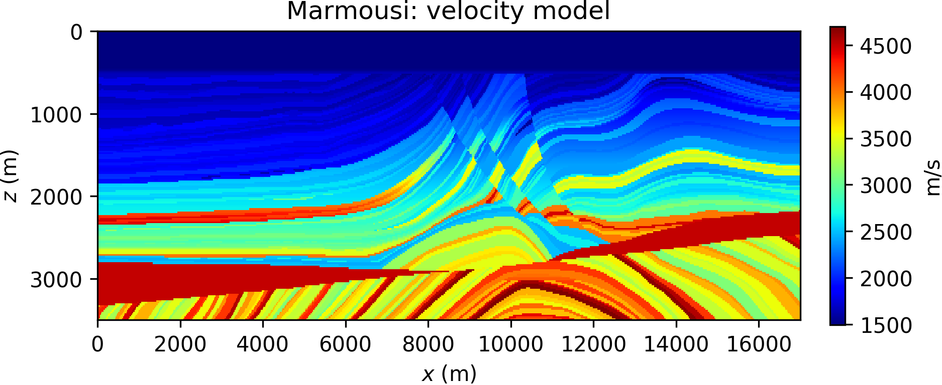
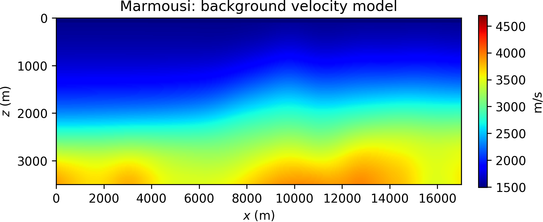
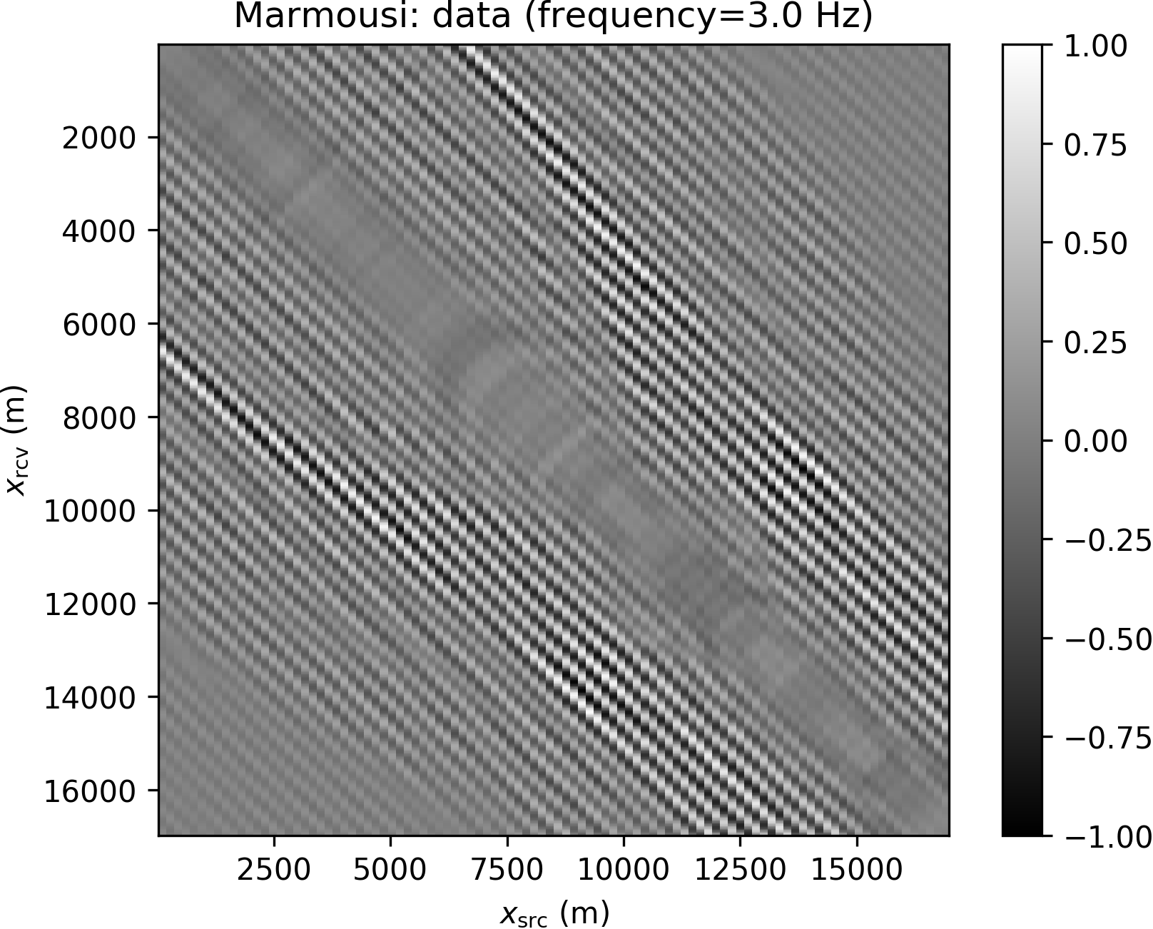
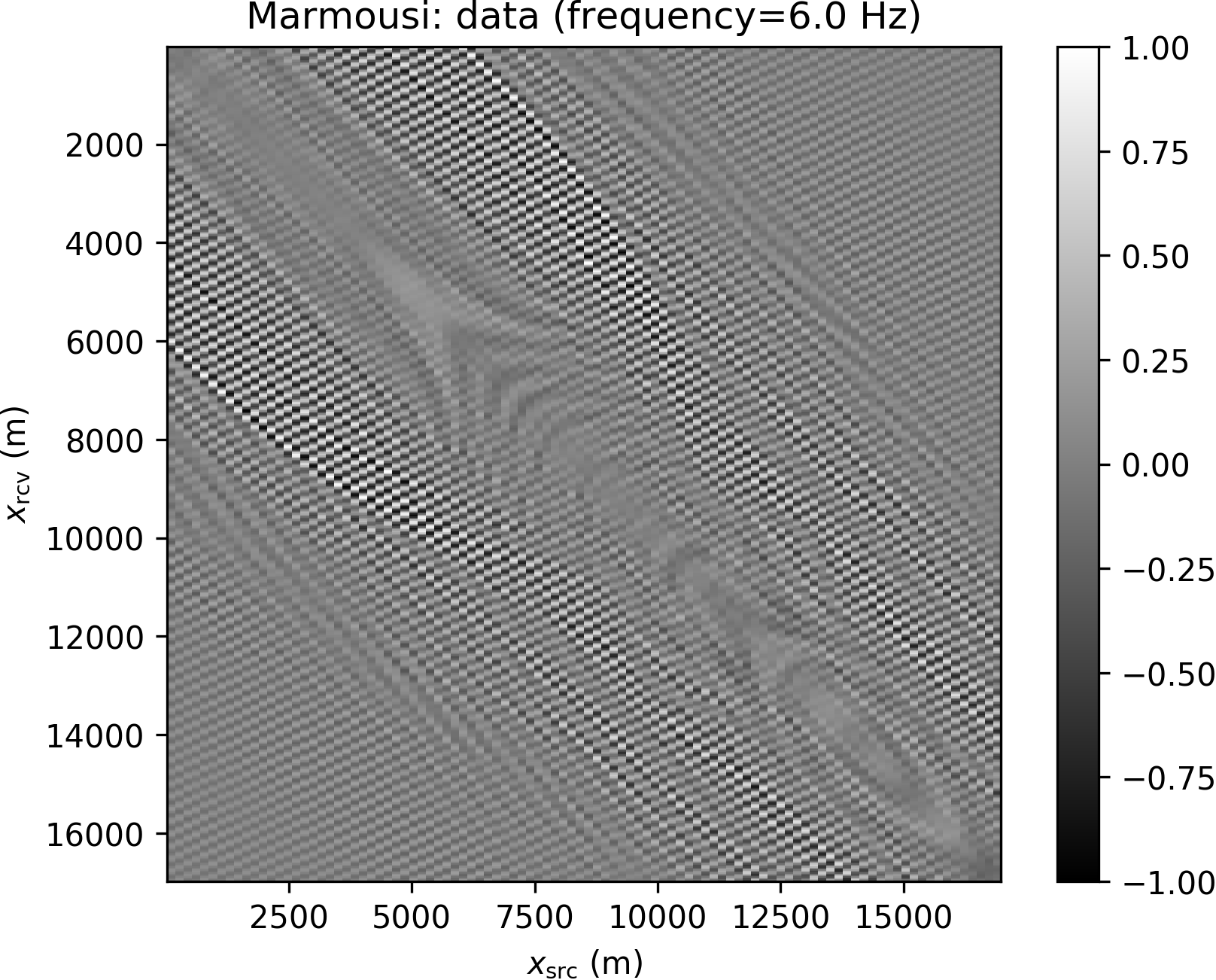
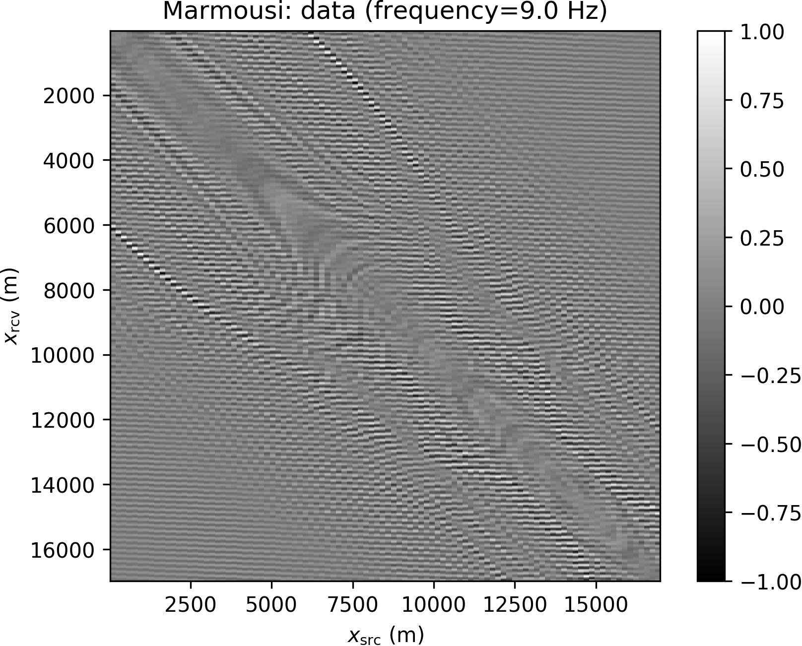
We consider the well-known Marmousi model, presented in Figure 1a. Data are directly generated in the frequency domain with components ranging from 3 Hz to 14 Hz, with no additional noise (Figure 2). We set 100 sources evenly spaced and receivers densely sampled along the surface.

We invert single-frequency data components with a multiscale approach (Bunks et al., 1995) from low to high frequencies, and run 10 iterations of the l-BFGS optimizer per frequency. We compare FWI, WRI\(\ast\) with different values for \(\epsilon\), and conventional WRI (with a fixed choice for the weighting parameter \(\lambda\) in equation \(\ref{eq:WRIdual_yopt_lin}\)). The results are gathered in Figure 3.

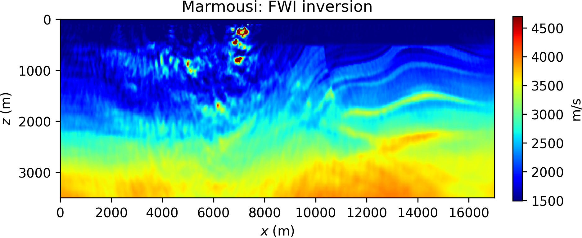
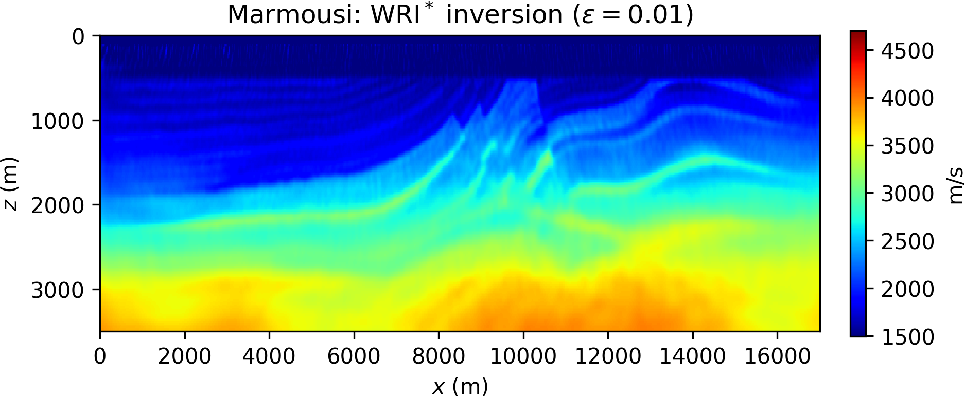
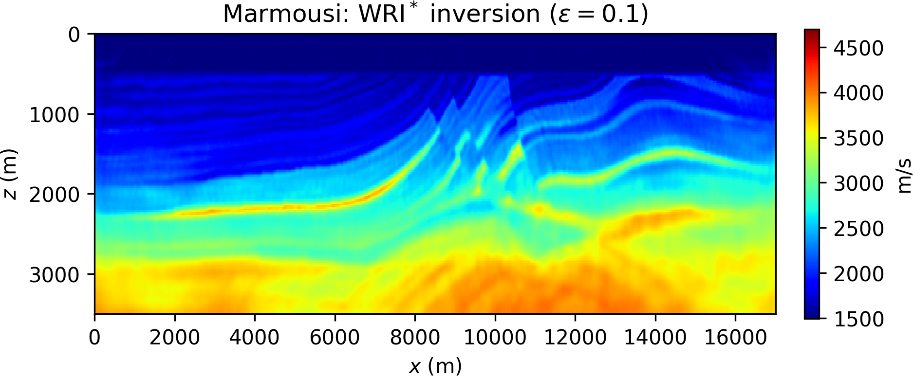
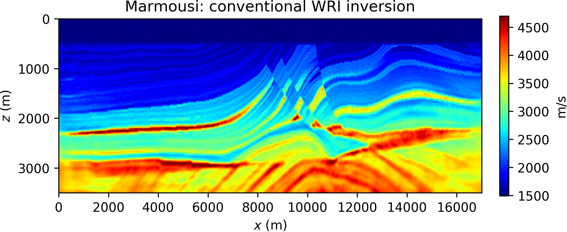
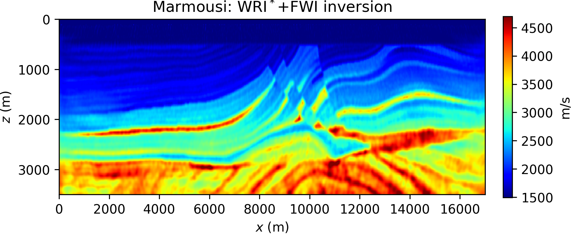
Comparing the results in Figure 3, it is apparent that FWI converges to a local minimum, while both WRI\(\ast\) and conventional WRI produce plausible models. WRI\(\ast\) does not achieve the same resolution of the WRI inversion, although we observe that increasing values for \(\epsilon\) translate to higher model resolution (cf. Figures 3b and 3c). This behavior can be understood in the following qualitative terms: lower values for \(\epsilon\) promote a wavefield solution that fits data rather than the wave equation (see, for instance, equation \(\ref{eq:denoise}\)), and unphysical solutions translate to inaccurate model resolution. This observation might seem in contradiction with the WRI result shown in Figure 3d: indeed the same considerations just made for WRI\(\ast\) should apply to WRI (where \(\lambda\) plays a similar role of \(\epsilon\)), and yet the WRI result consists in a much better resolved model. This paradox is due to the notorious well-conditioning properties of variable projection (Golub and Pereyra, 2003): WRI\(\ast\) has been obtained through only an approximation of the optimal dual variable \(\by\), and therefore does not enjoy the same advantages of WRI. In general, however, WRI\(\ast\) conserves the same ability of WRI to circumvent local minima, and the gap between the two methods can be reduced by either quasi-Newton preconditioning or devising a sequential WRI\(\ast\)-FWI scheme where the WRI\(\ast\) result is sharpened by FWI (which will also help in saving computations once local minima are avoided). An example of the joint WRI\(\ast\)-FWI approach is depicted in Figure 4, highlighting a qualitatively similar result to conventional WRI in Figure 3d.

Comparison of FWI and WRI\(\ast\)

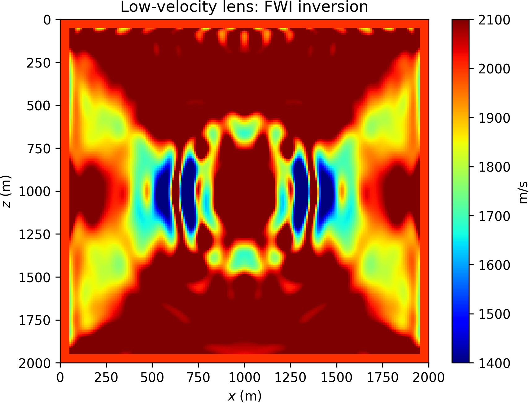
Low-velocity lens

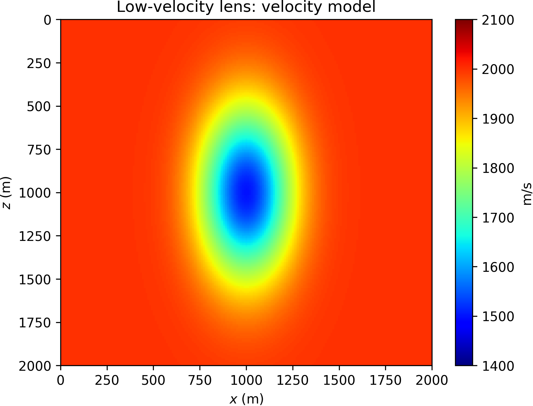
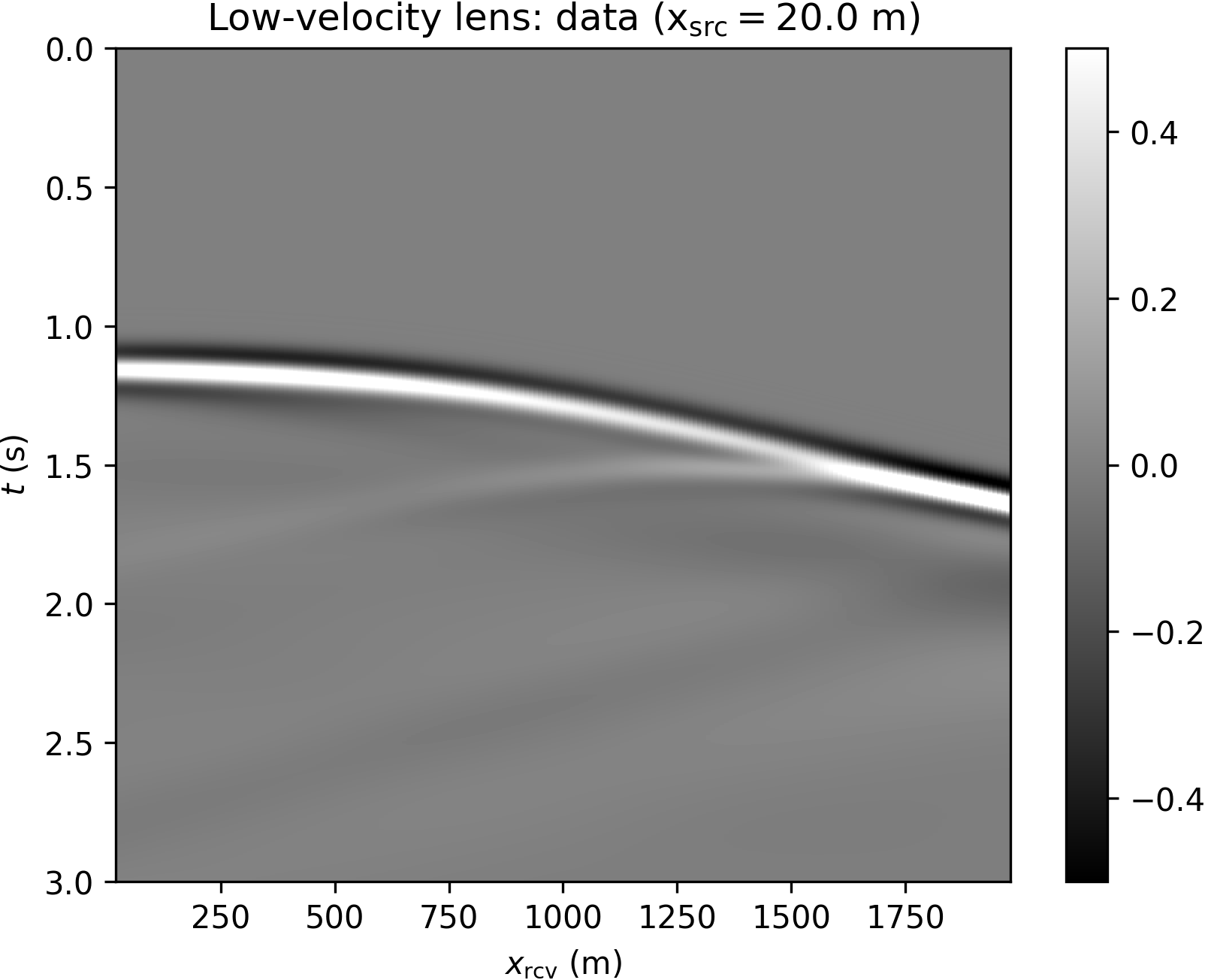
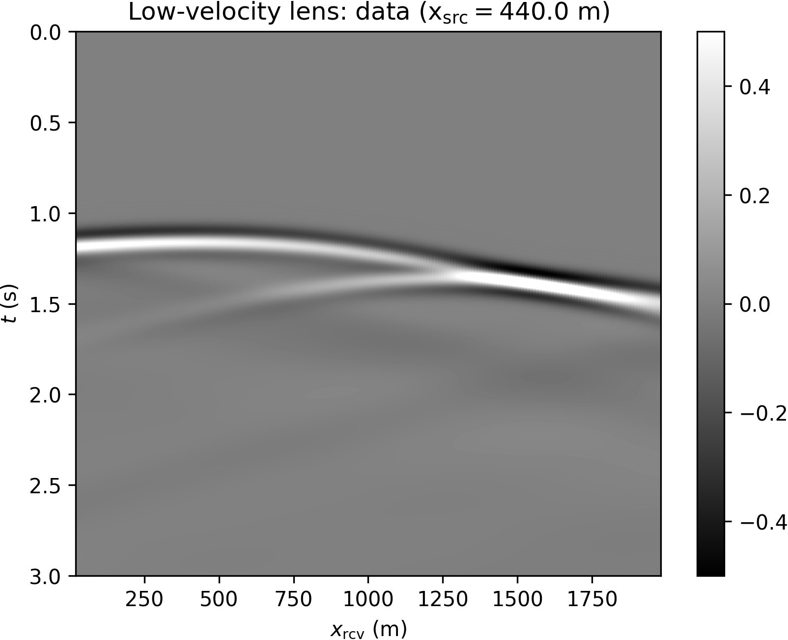
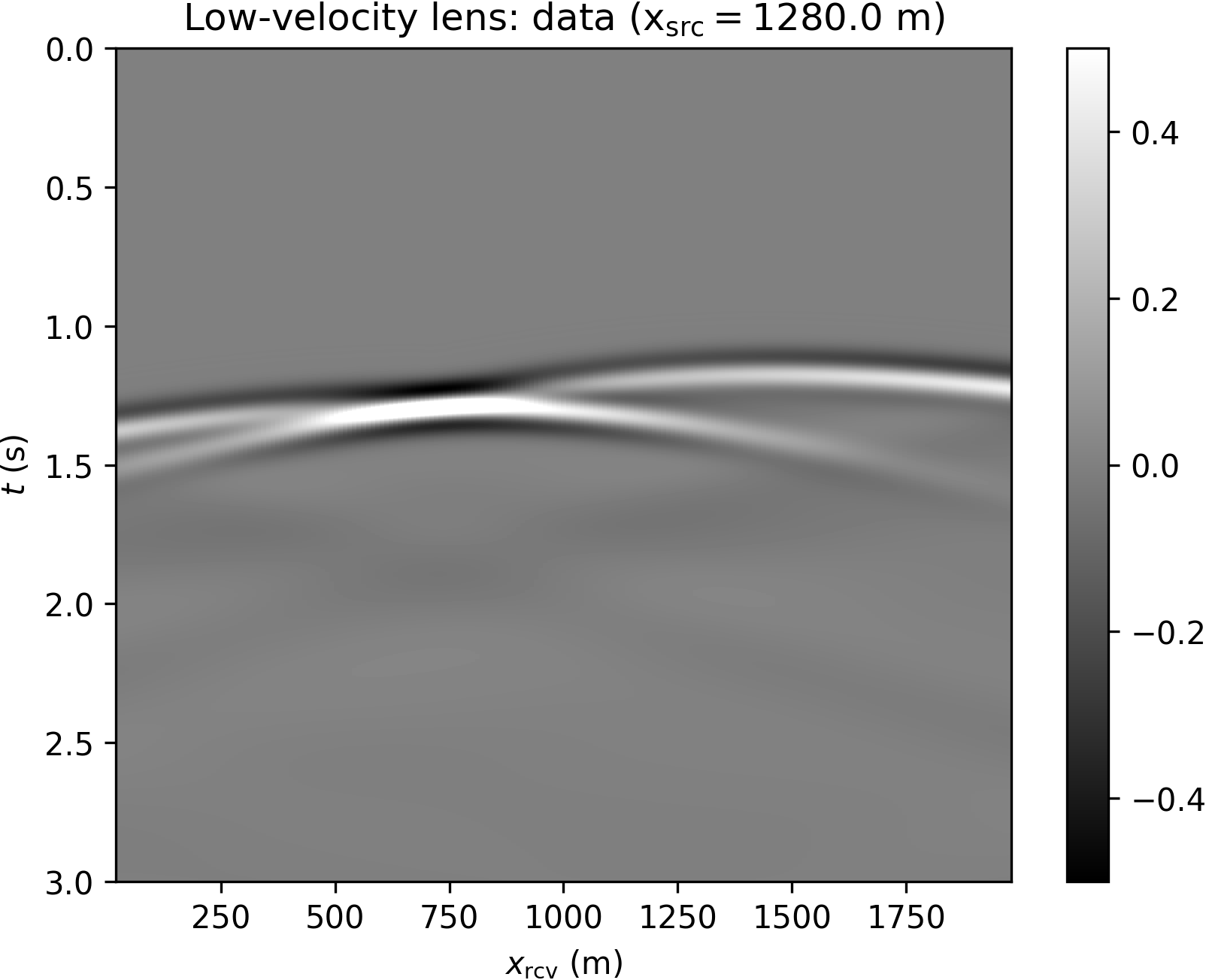
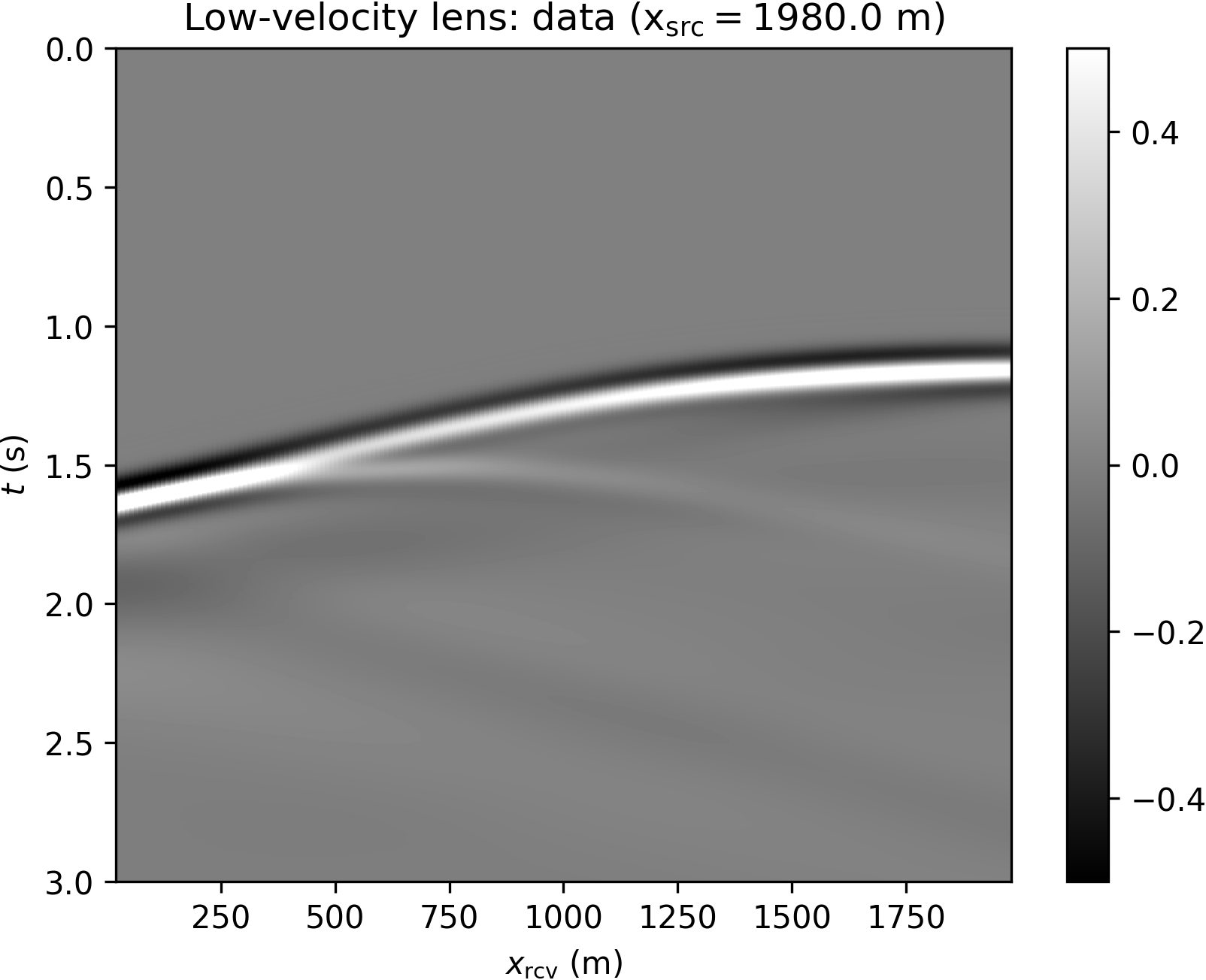
This numerical experiment is geared towards a direct comparison of WRI\(\ast\) and FWI, and demonstrates the relative robustness of WRI\(\ast\) against spurious modes. We consider the Gaussian lens model presented in (Huang et al., 2018), here reproduced in Figure 5. The problem consists of imaging a low-velocity anomaly of Gaussian shape from transmission data, starting with an homogeneous model. Contrary to the previous example, we run this experiment in time domain. The synthetics are generated with a Ricker source wavelet of 10 Hz peak frequency (corresponding to a spatial wavelength of 200 m), with no artificial noise added. We model 15 sources, and gather data with approximately 200 receivers (evenly spaced). The low-velocity zone generates triplications that are apparent in the data shown in Figure 6, which cause cycle skipping.

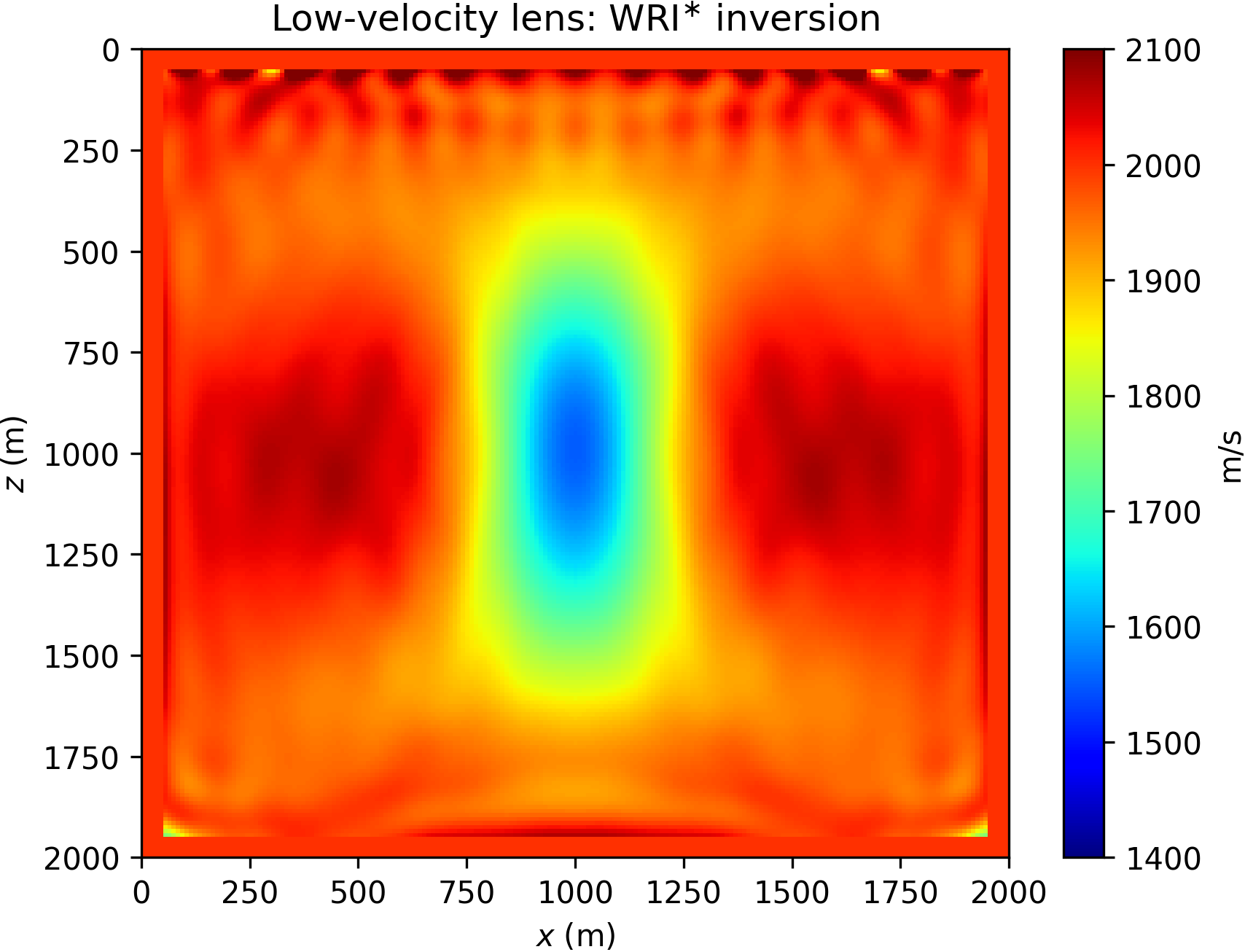
In this experiment, we run 20 iterations of the l-BFGS optimizer (Nocedal and Wright, 2006). Due to cycle skipping, FWI converges to a local minimum, shown in Figure 7b. We stress the fact both WRI or WRI\(\ast\) need be used in combination with source weighting (equation \(\ref{eq:srcweight}\)) to converge to the solution (as also documented in Huang et al., 2018; Symes, 2020a, 2020b). The WRI\(\ast\) result (obtained with data tolerance \(\epsilon=0\)) is depicted in Figure 7a. We observe that WRI\(\ast\) is clearly able to reconstruct the anomaly and is not stuck to a local minimum, contrary to FWI.

BG Compass

We focus now not only on how WRI\(\ast\) and FWI handle cycle skipping, but also how inaccurate assumptions about the underlying physical model of the data reflect on the inversion result. For example, what is effect of not accounting for the correct anisotropic model when data come from anisotropic modeling? We show that WRI\(\ast\), being based on a relaxation of the wave equation, has the potential to mitigate erroneous assumptions, while FWI will be more heavily affected. We therefore compare the results of WRI\(\ast\) and FWI on the BG Compass model according to two distinct scenarios:

• perfect modeling assumptions: both given data and modeled synthetics are obtained from the same physical model (in particular, acoustic modeling). The inversion parameter is the squared slowness;
• inaccurate modeling assumptions: given data are produced with a certain TTI model (tilted transverse isotropy), while synthetics are modeled with an inaccurate TTI model. All the TTI parameters but the squared slowness are kept fixed during inversion.

As in the previous example, this set of experiments is carried out in time domain.

Inversion with correct modeling assumptions

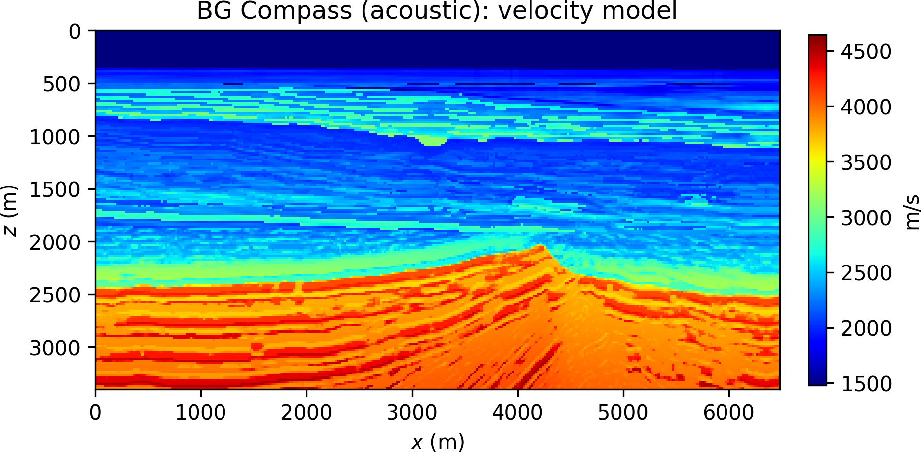
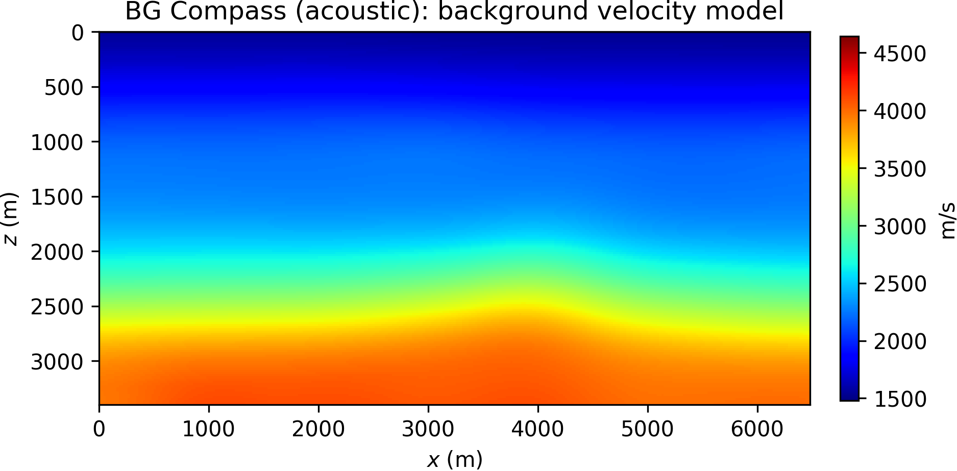
The acoustic (constant density) BG Compass model, here considered, is representative of some of the complexities encounter in the field, and leads to a notoriously challenging problem for FWI due to the velocity kickback approximately located at the depth of 1 Km (see Figure 8), delaying turning waves traveling back to the surface.

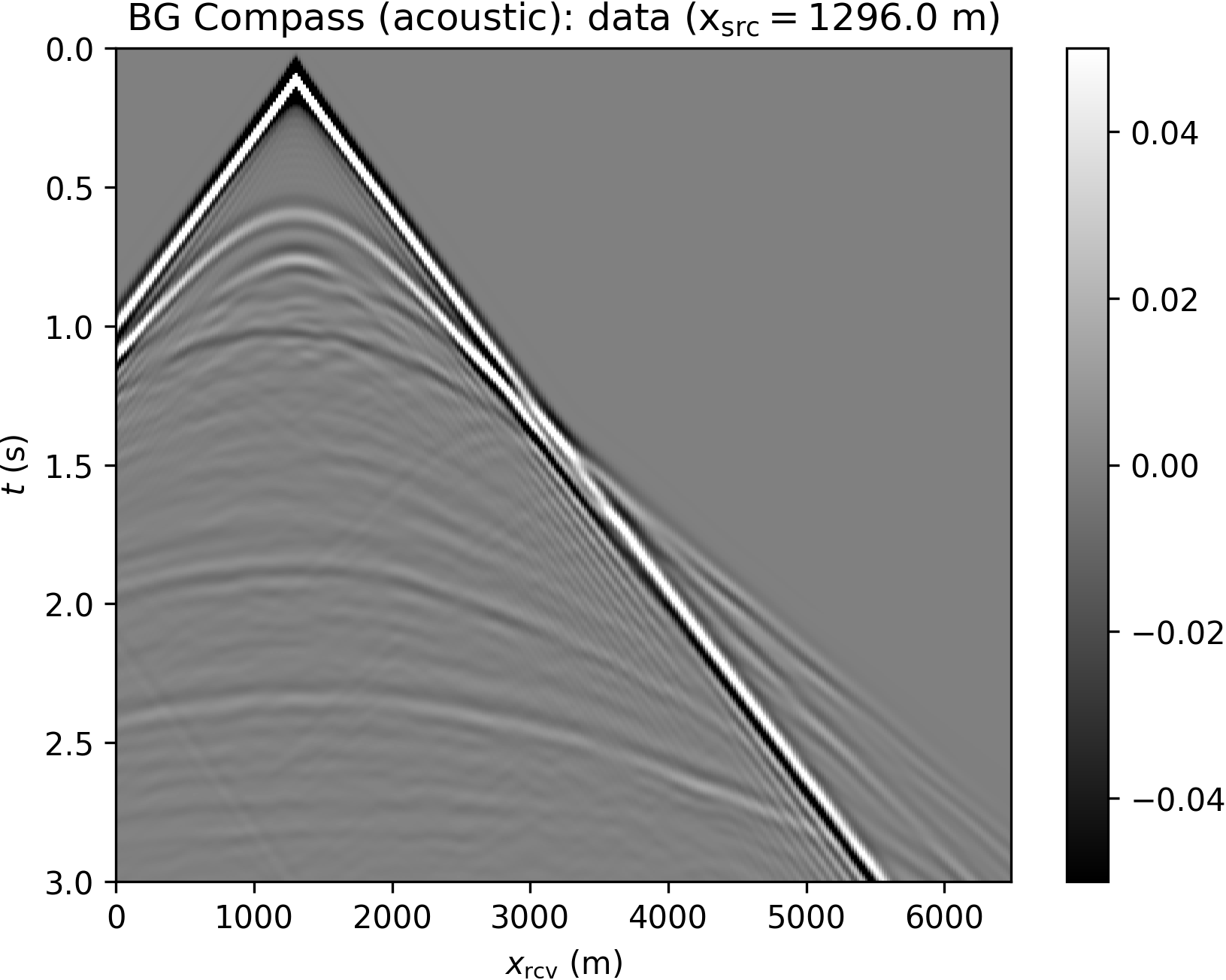
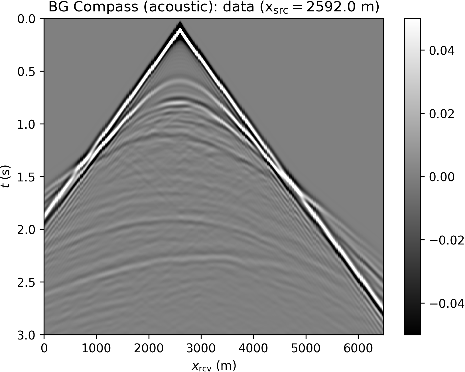
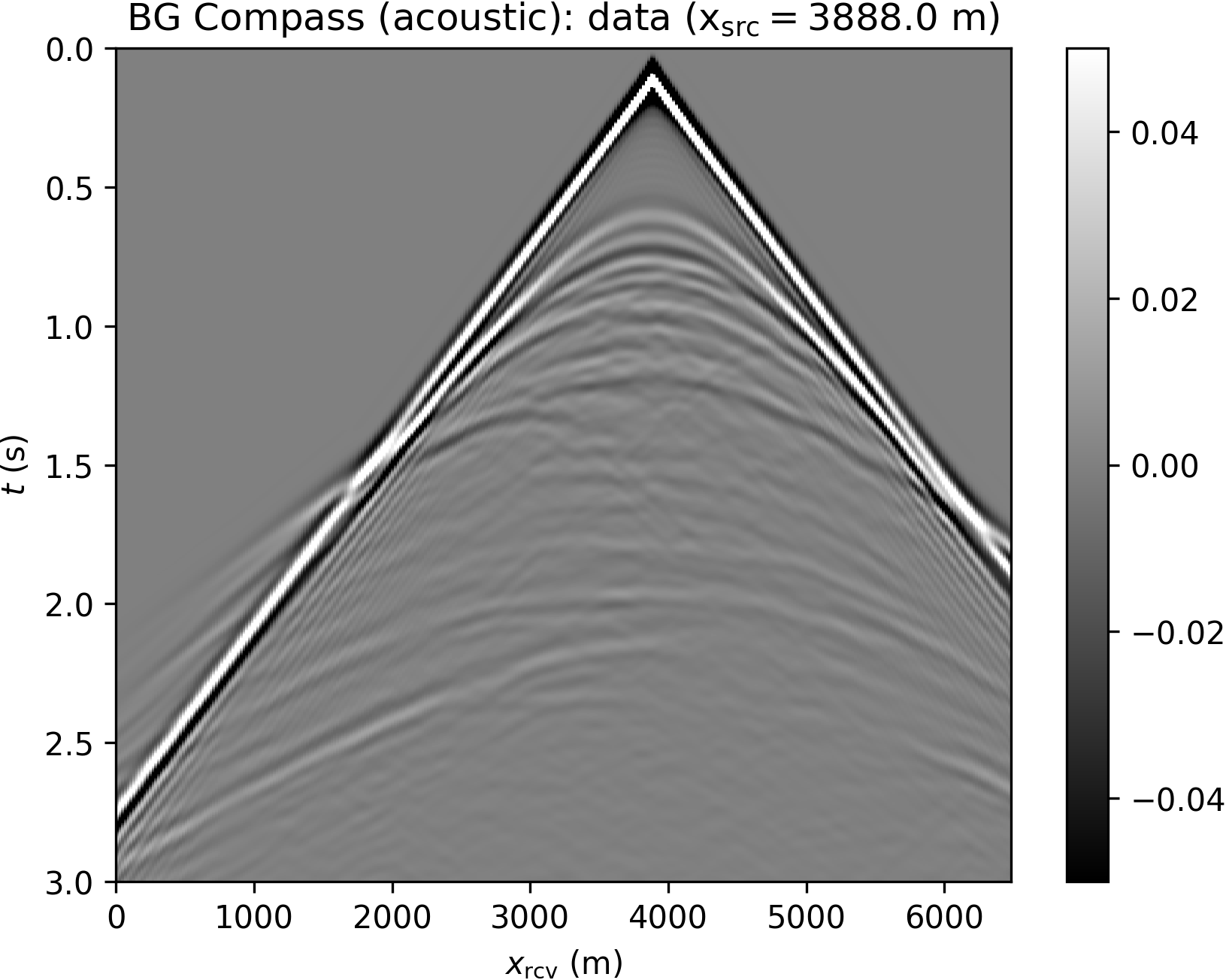
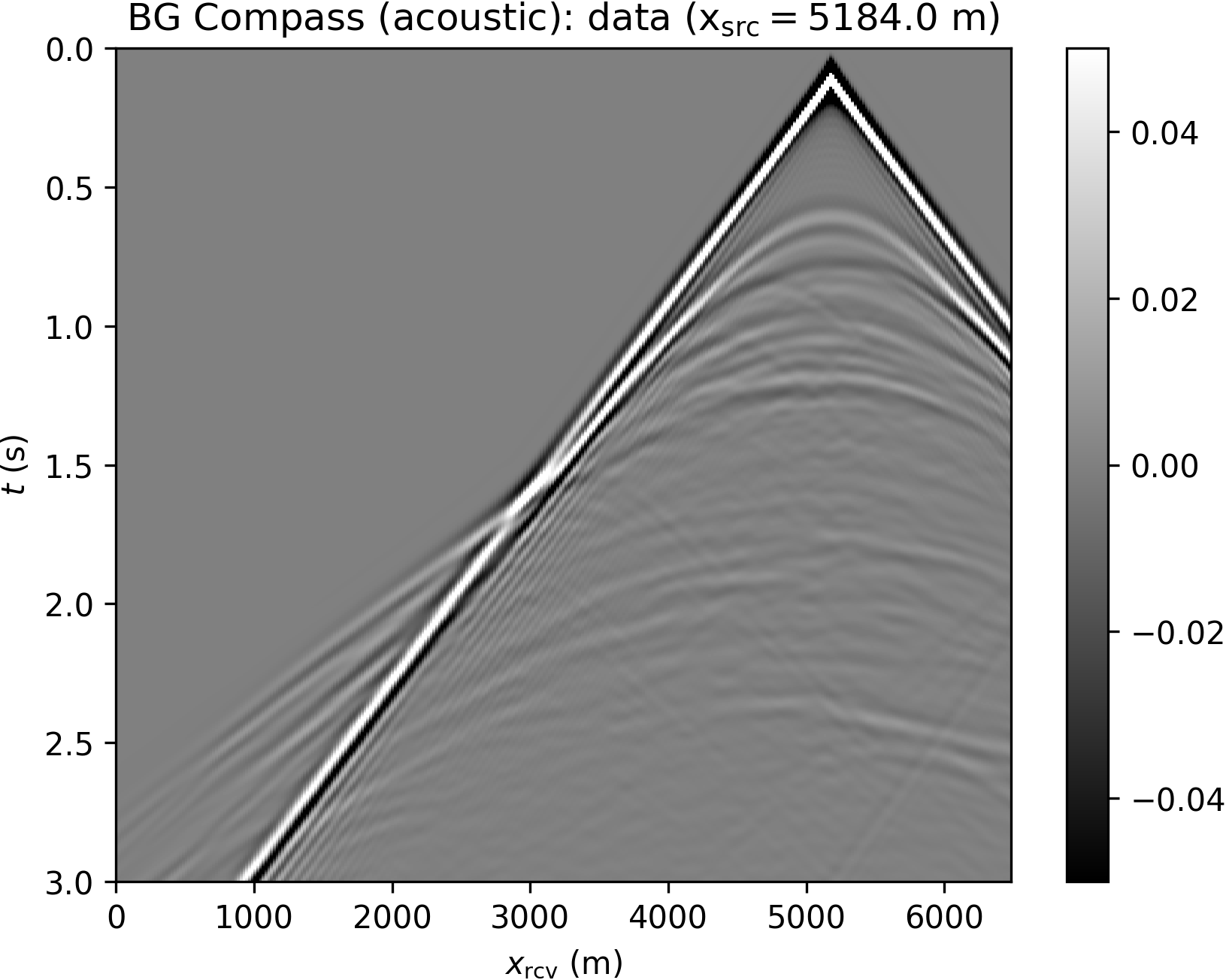
We model 51 sources with a Ricker wavelet (peak frequency 10 Hz), and record data with dense receiver coverage (sampling rate according to the grid spacing), without additional noise. Some shot records are plotted in Figure 9. Note that the frequency components below 5 Hz in the data are filtered out and not used during inversion.

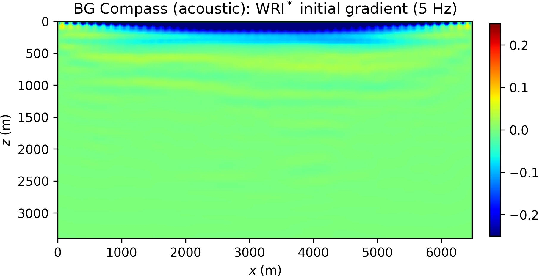
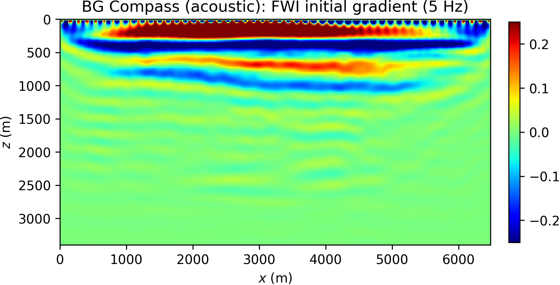
The difficulties associated with the BG Compass model are hinted in Figure 10, where the squared slowness gradients of WRI\(\ast\) and FWI (computed with respect to the background model in Figure 8b) are compared. These are obtained by filtering the data according to a narrow frequency band centered at 5 Hz (a similar result can be obtained by working directly in the frequency domain, B. Peters et al., 2014). We observe that FWI produces an erroneous update in the water layer, while WRI\(\ast\) points in the correct direction.

For the inversion, we adopt a multiscale strategy (Bunks et al., 1995), by filtering and inverting data components of increasing frequency content, from 5 Hz to 20 Hz. This is achieved by preconditioning both data and synthetics. For simplicity, we do not adapt the model grid to the varying frequency. At each of these sequential stages, we perform l-BFGS optimization for 20 iterations and use the result as the starting guess for the next step. The process is repeated with multiple sweeps across the frequency range, by repeating the multiscale inversion twice and restarting from the lowest frequency when the first pass is completed. The final results for WRI\(\ast\) and FWI are collected in Figure 11. For reference, see also B. Peters et al. (2014) for frequency-domain WRI inversion results on a similar model.

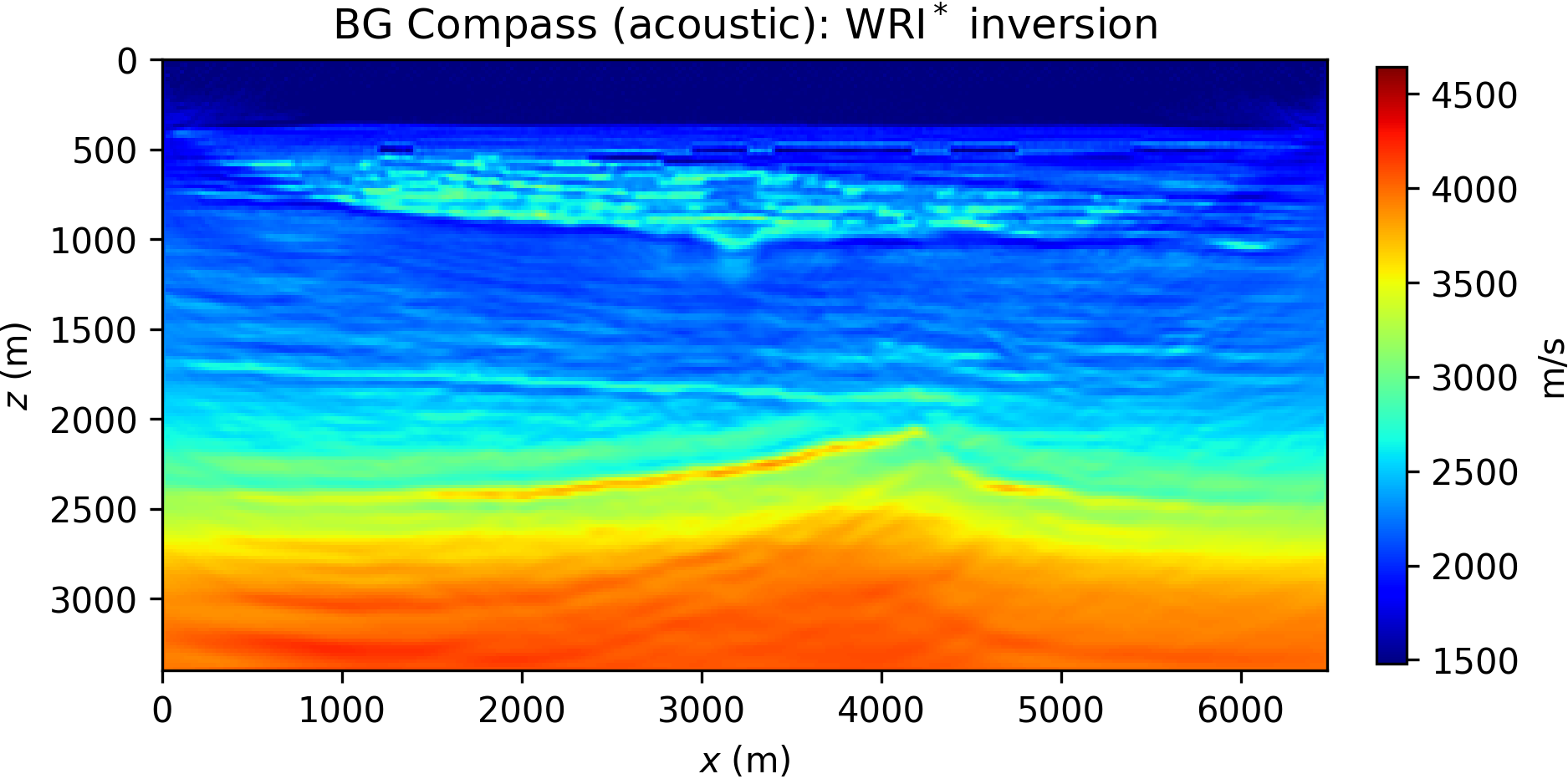
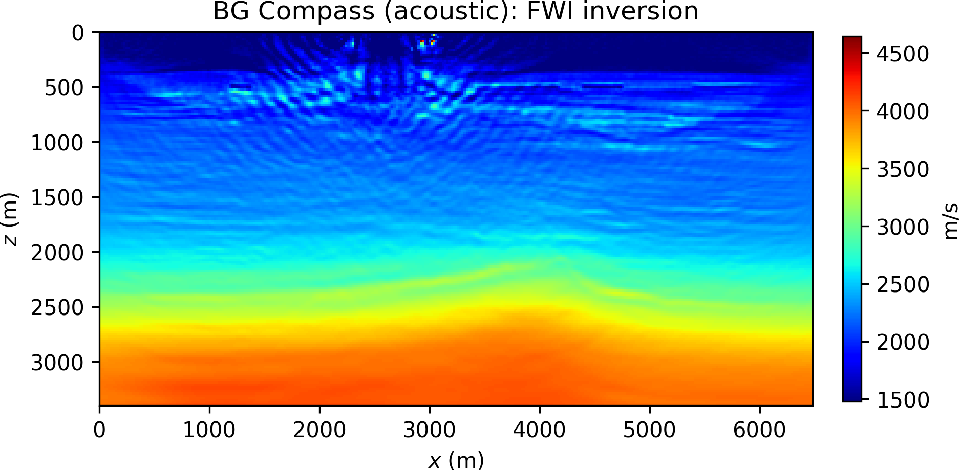
Notably, the poor update generated by FWI within the water layer eventually leads to the local minimum in Figure 11b (for FWI, we report the result after only one data sweep). The WRI\(\ast\) result (with data tolerance \(\epsilon=0\)) is shown in Figure 11a. Clearly, WRI\(\ast\) is able to correct for the water layer and resolve the high-velocity/low-velocity sequence at 1 Km depth. The deeper part of the model can be improved, in principle, by further optimization or pseudo-Hessian preconditioning via incident field energy (see van Leeuwen and Herrmann, 2013 for a simple Gauss-Newton scheme).

Inversion with inaccurate modeling assumptions

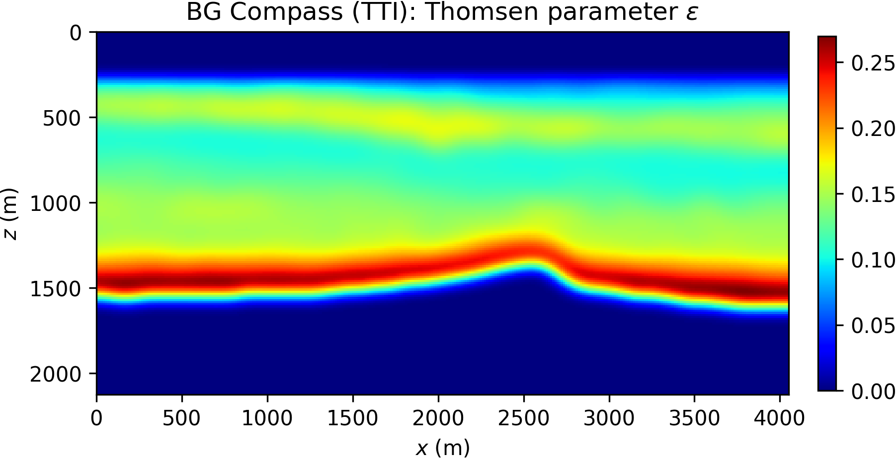
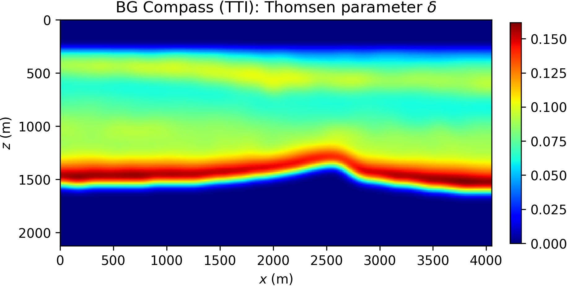
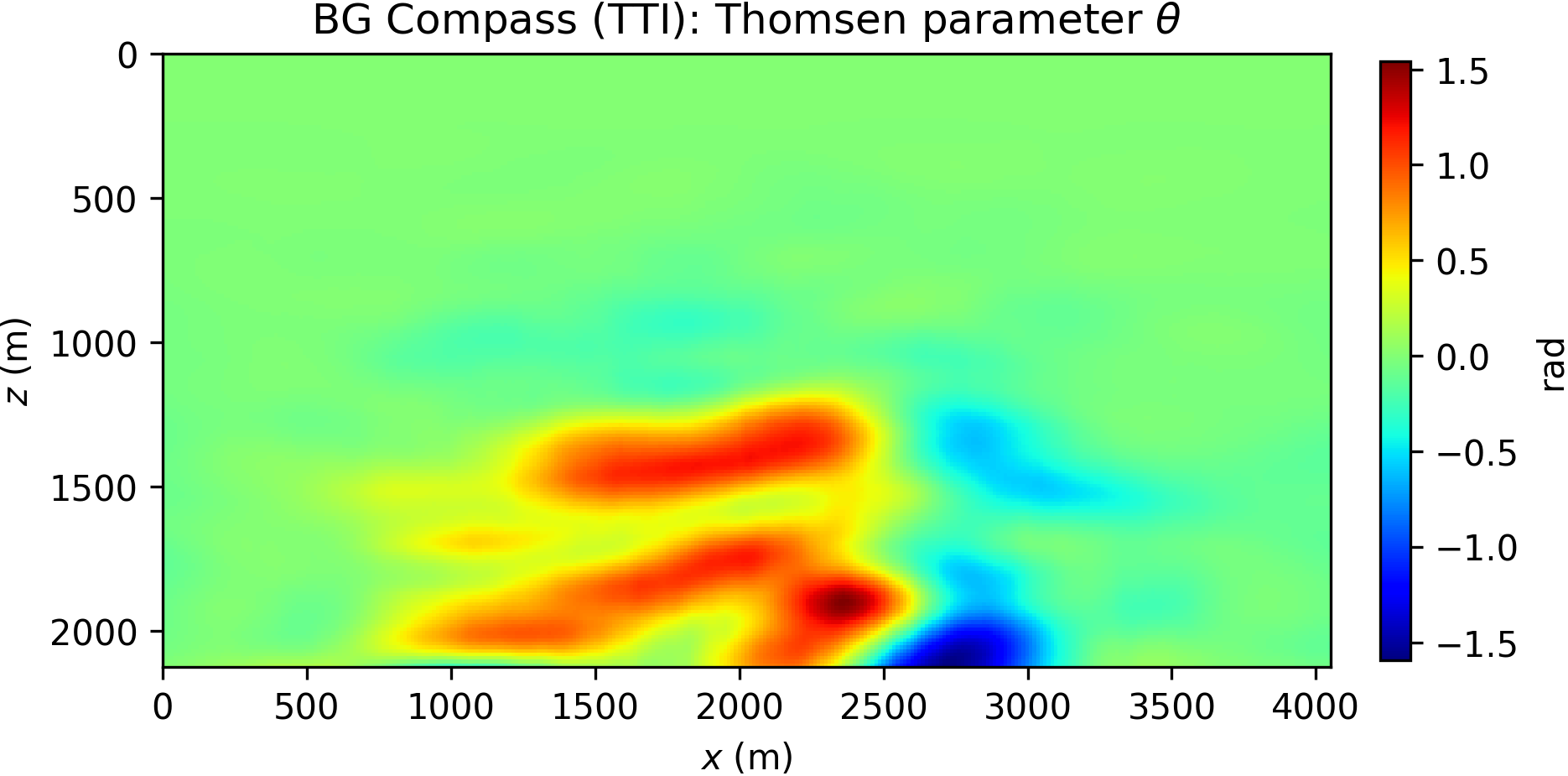
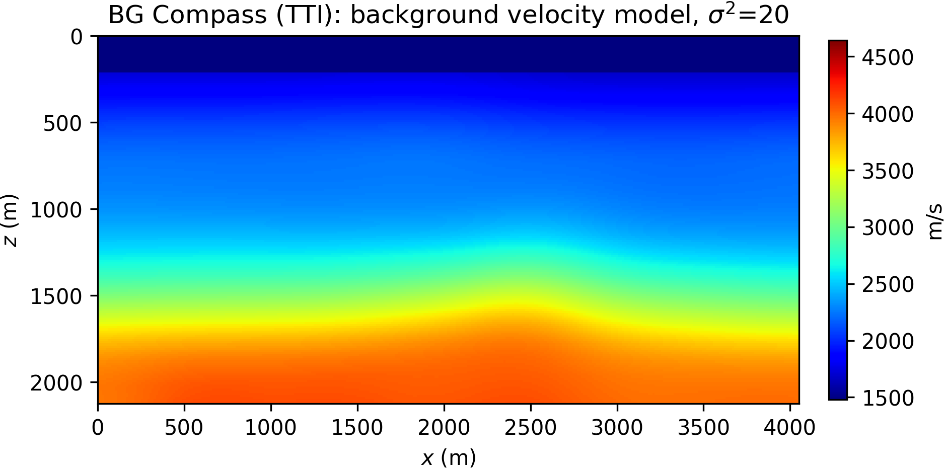
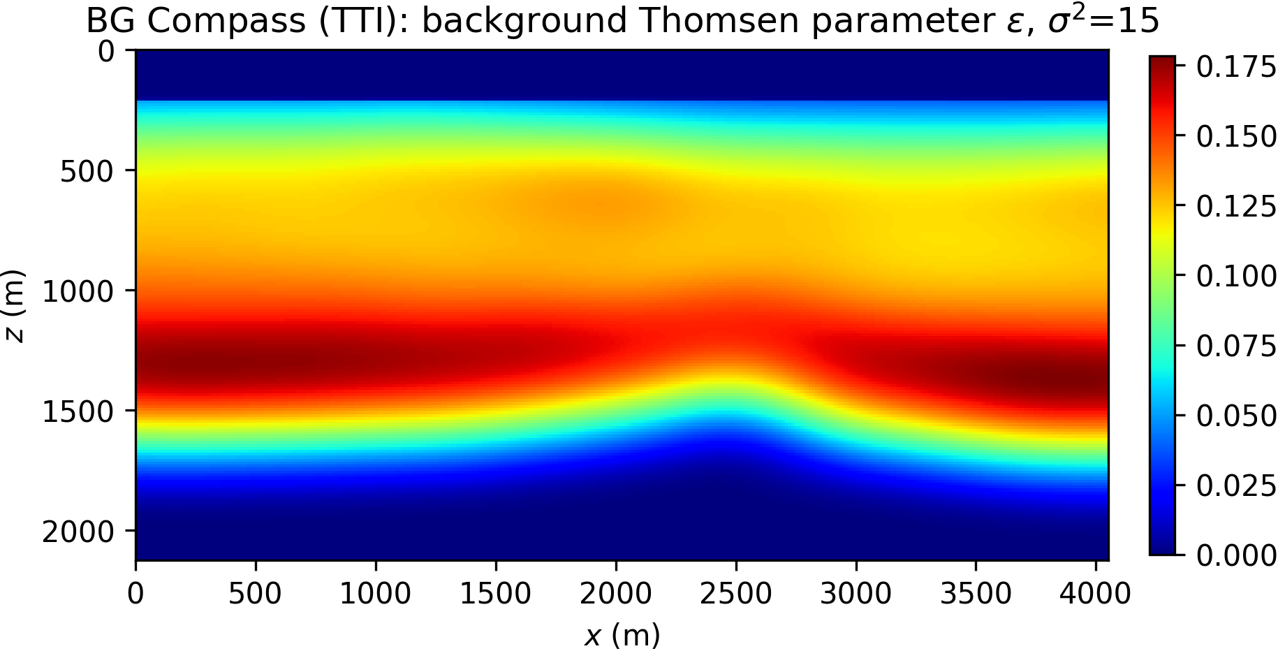
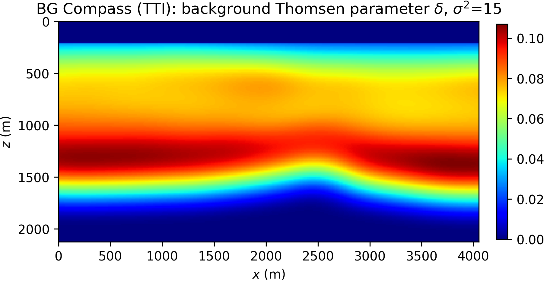
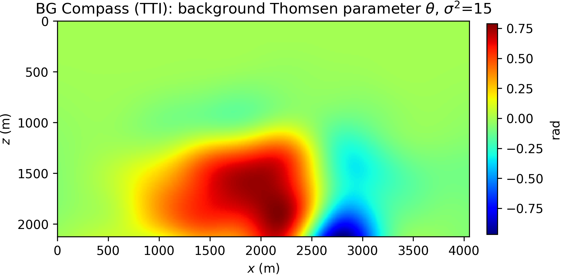
Here, we consider a TTI anisotropic version of the acoustic BG Compass model, previously shown in Figure 8a. The model is rescaled for practical reasons. The Thomsen parameters \(\varepsilon\) and \(\delta\) are synthesized from the velocity model, and dip angles inferred from the orientation of the layers. The TTI model is presented in Figure 12.

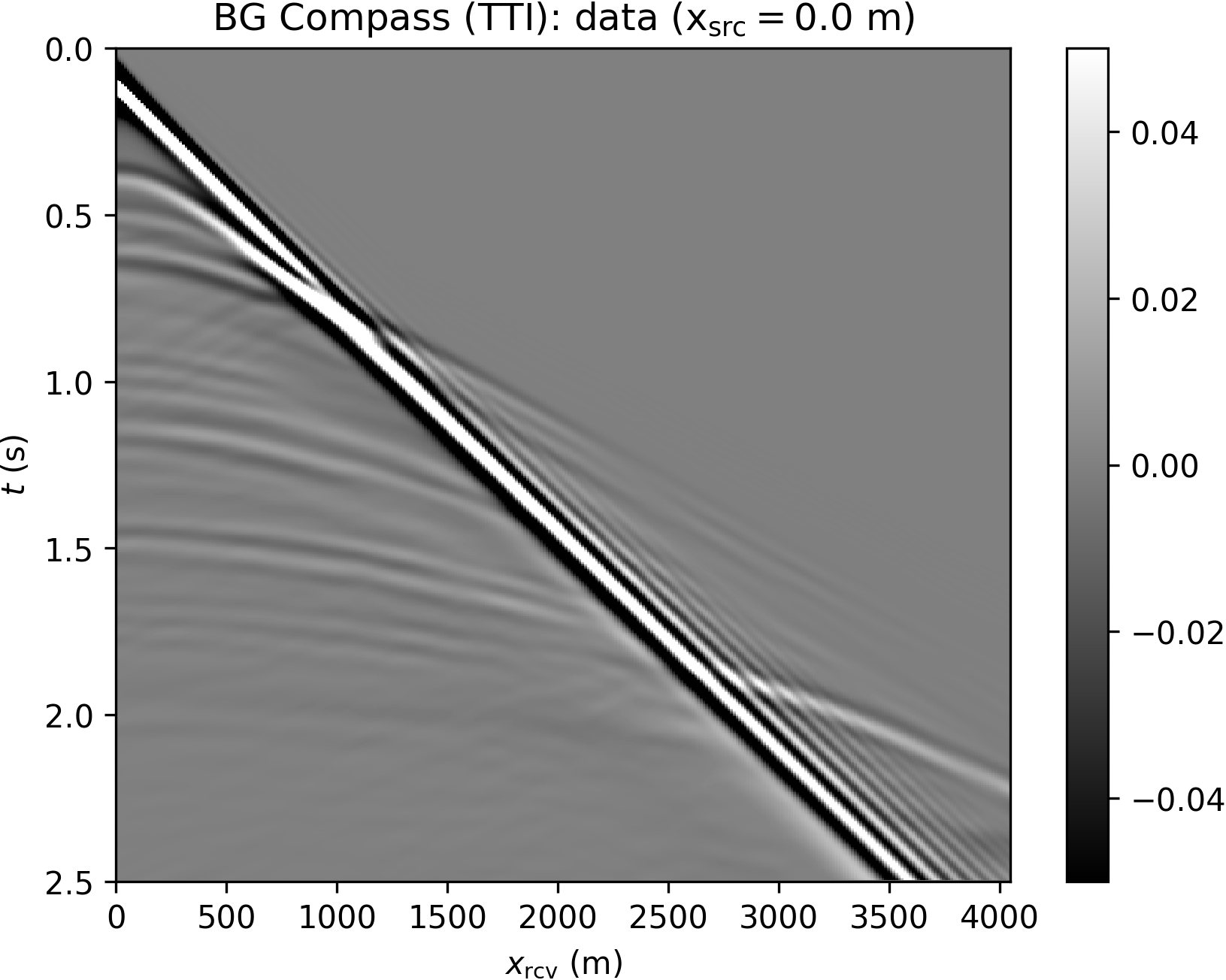
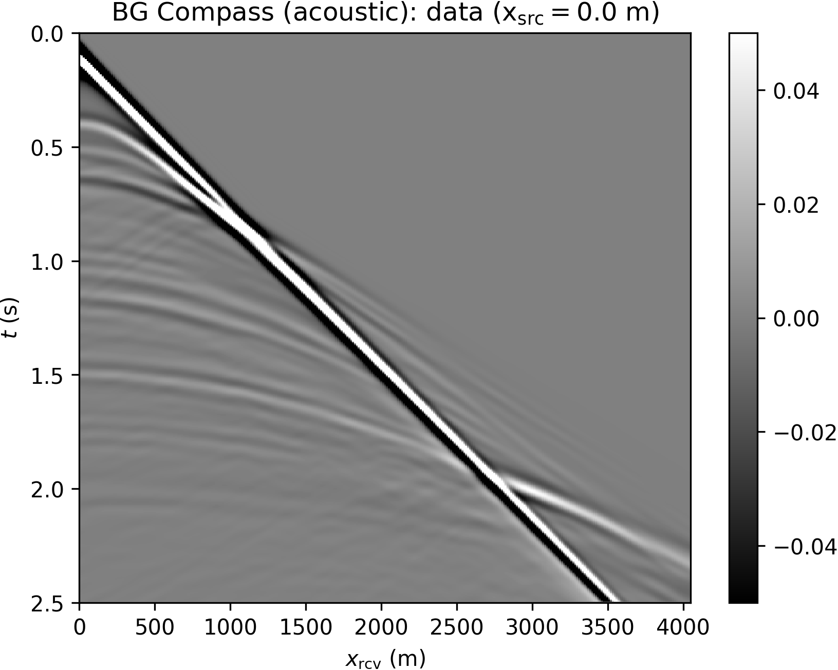
Data are generated according to the same settings described for the acoustic BG Compass model (note, however, that the TTI model size is different). In order to illustrate the effect of anisotropy, we compare acoustic and TTI shot gathers in Figure 13, highlighting arrival times differences for both turning wave and reflection events.

The inversion is performed with data generated with a Ricker wavelet of peak frequency 10 Hz (with low frequencies filtered out), and the optimization is carried out by 20 iterations of the spectral projected gradient method (SPG) of Birgin et al. (2000) (the projection here bounding velocity values). We compare the robustness of the WRI\(\ast\) and FWI results by initializing the inversion with increasingly worse smoothed version of the true velocity model. The anisotropic parameters are smoothed and kept fixed for all the experiments and throughout the inversion. The inconsistency between true and assumed TTI parameters will be the source of modeling inaccuracy with which we test the resilience of the velocity model recovery with WRI\(\ast\) and FWI. An example of TTI model with smoothing level \(\sigma^2=20\) (indicating the variance of Gaussian smoothing) is depicted in Figure 14.

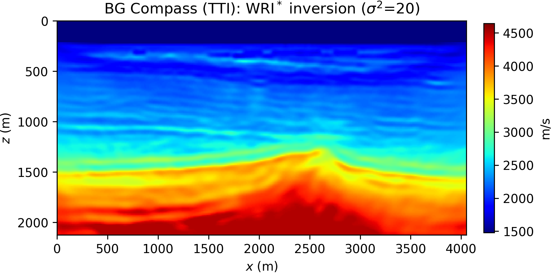
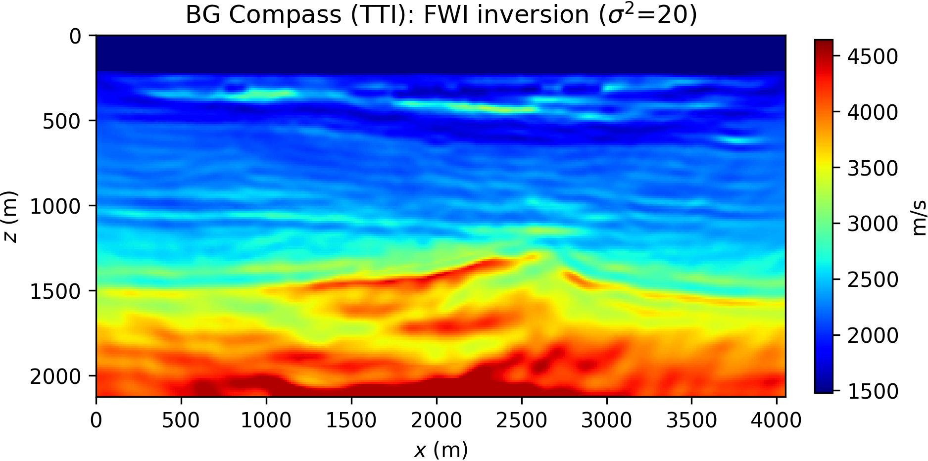
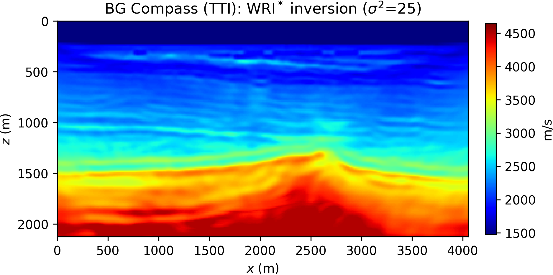
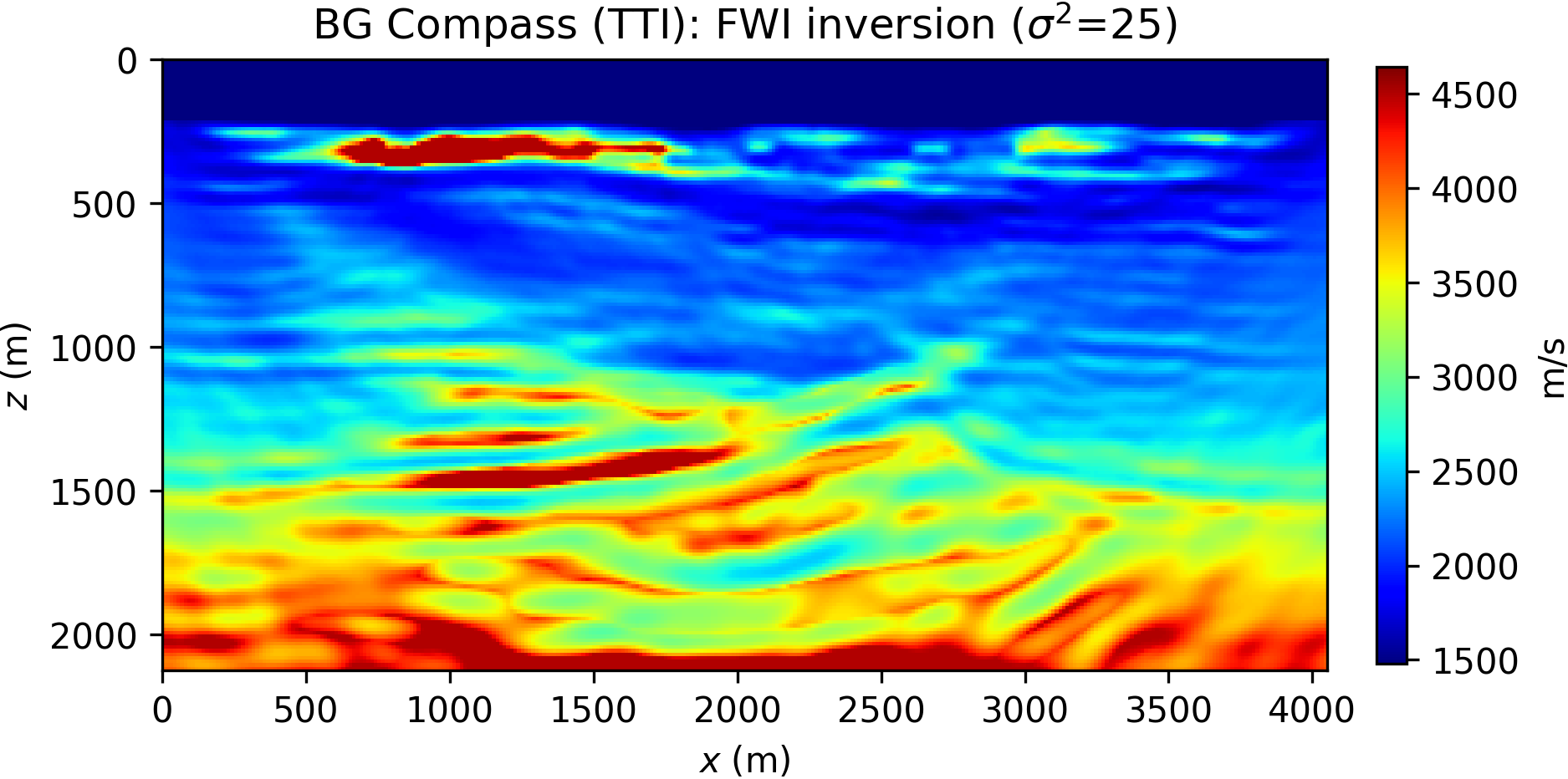
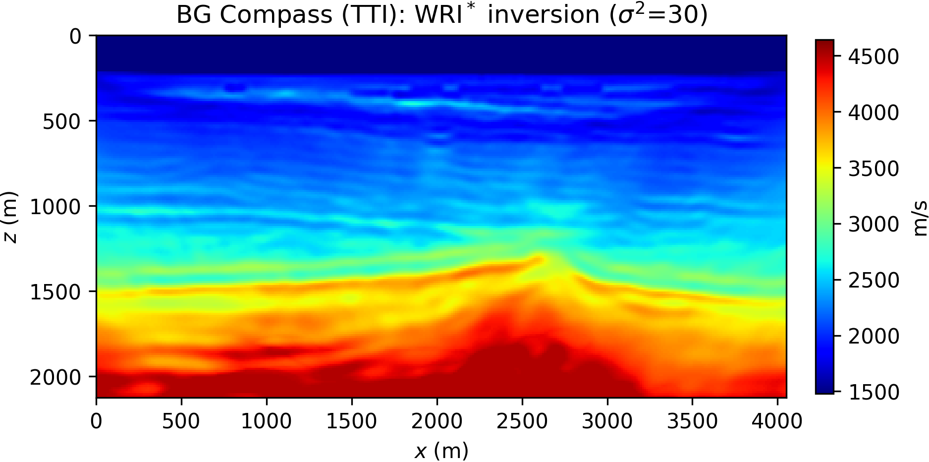
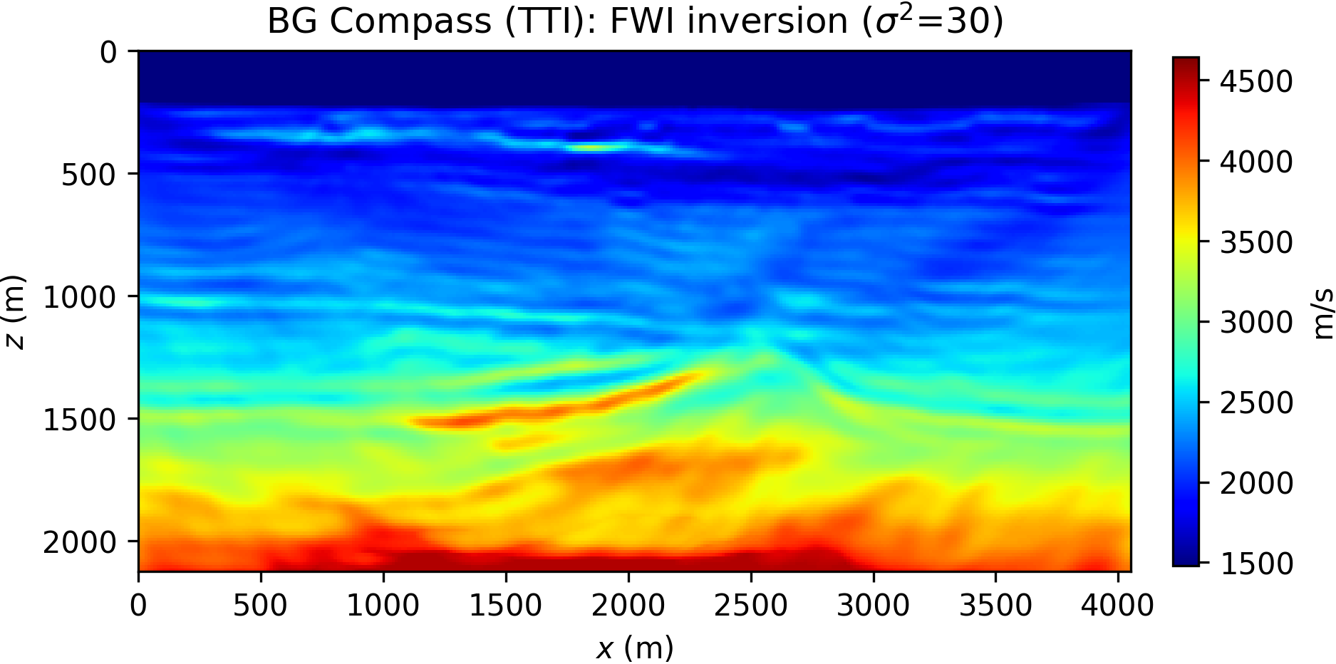
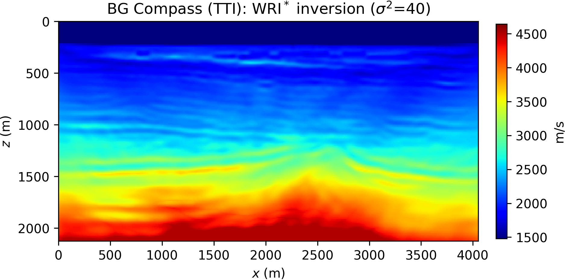
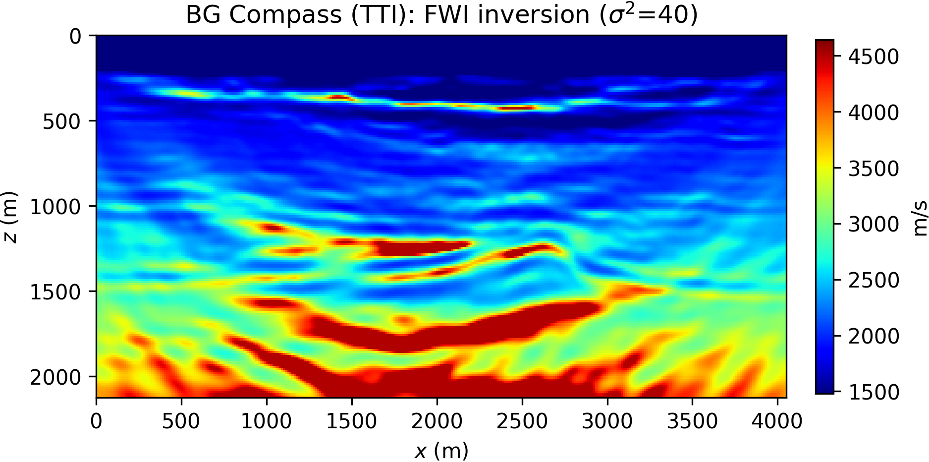
The inversion results for WRI\(\ast\) and FWI are displayed in Figure 15. We notice that the starting model and wrong assumptions about anisotropy have an effect on WRI\(\ast\) results, especially in resolving the shallow high-velocity layer and the deeper part of the model. Despite this, the WRI\(\ast\) results remain relatively stable with respect to the starting guess, the major difference being a loss of resolution with depth with worse starting models. More notably, they are consistently better than the FWI results, which are instead heavily affected by this choice.

Discussion

The application of modern seismic inversion tools to field data has been curbed by the need for tremendous computational resources, which are required for wave simulations on extremely large 3D grids. Moreover, classical acoustic models are gradually being discarded in favor of pseudo-acoustic or elastic simulators to account for anisotropic phenomena in field data. Less simplistic modeling inevitably adds to the computational complexity of the problem. Be that as it may, the oil and gas industry manages to employ FWI almost on a routinely basis, thanks to efficient time-domain simulators, and its business value is starting to be acknowledged. Unfortunately, the success of FWI is highly dependent on a lengthy preprocessing phase aimed at the retrieval of a kinematically accurate background and starting guess for seismic inversion.

The main objective of this work is to dispense of the need for accurate velocity models in seismic inversion. Despite the fact that many solutions exist focusing on robustness with respect to local minima, they do not scale efficiently with grid size and are not relevant for real-world applications. One such example is WRI. WRI is, nonetheless, an attractive method that is not only robust with respect to the starting guess, but also has the potential to handle inexact physical assumptions. Indeed, WRI hinges on a relaxed wave equation, whose solution, however, can only be approximated iteratively in 3D with considerable computational costs.

We presented a novel method, WRI\(\ast\) which is both scalable and robust. It is based on a denoising reformulation of WRI, which amounts to the minimization of the wave equation error subject to the data misfit being less than a known noise level. The resulting saddle-point problem involves the usual model unknowns, such as squared slowness, and Lagrangian multipliers having the same dimension as data. We stress that all the computations needed for the evaluation of the Lagrangian and its gradients require modeling in time domain, which can be attained for realistically sized problems (contrary to frequency domain formulations). Since the dual variables can be stored in memory, we might in principle devise a joint optimization scheme. In this paper, however, we approximate the Lagrangian multipliers with a scaled version of data residual in order to reduce complexity (a more accurate assessment of the trade-off between multiplier approximation and reconstruction quality is left for future studies).

We demonstrated, through extensive numerical experimentation, that the resulting method is consistently more robust than FWI against local minima. We also tested the tolerance of the method toward faulty modeling assumptions, e.g. when seismic data obtained with anisotropic modeling is being matched with predictions based on the wrong anisotropic model. WRI\(\ast\), which employs a relaxation of the wave equation, produces better results than FWI, under the same conditions.

In general, the results obtained from WRI\(\ast\) do depend on the particular choice of hyperparameters such as the data noise level \(\epsilon\), defined in equation \(\eqref{eq:denoise}\). This parameter governs the trade-off between wave equation error and data misfit and is akin to the role of the weighting parameter \(\lambda\), in equation \(\eqref{eq:WRI}\), for conventional WRI. We find that decreasing its value tends to produce lower resolution results. On the other hand, choosing a small value for \(\epsilon\) (or even \(\epsilon=0\)) results in relaxed physics and is beneficial for local minimum avoidance. In our experience, WRI\(\ast\) retains the same ability of WRI to circumvent local minima, but might produce less qualitative results, especially in terms of resolution. We note that conventional WRI is not as affected as WRI\(\ast\) by the choice of \(\lambda\). The fundamental reason for this phenomenon is rooted in the inexact, but relatively inexpensive, dual variable approximation in equation \(\eqref{eq:alpha}\), as opposed to equation \(\eqref{eq:WRIdual_yopt}\). Indeed, WRI\(\ast\) does not enjoy the well-conditioning properties of variable projection (Golub and Pereyra, 2003). Taking into account the dependency of the approximated dual variable with respect to the model parameter, as in equation \(\eqref{eq:WRIdg_gradm_corr}\), is designed to partially compensate for this behavior (Ablin et al., 2020). We then advocate for either a continuation strategy for \(\epsilon\), by increasing its value sensibly during the inversion, proper preconditioning (as in the Gauss-Newton approach in van Leeuwen and Herrmann, 2013), or a sequential approach consisting of a WRI\(\ast\) phase followed by FWI. Preliminary results prove this strategy successful. Another approach might consist of iteratively solving for the optimal dual variable, but we envisage this can be only feasible in combination with stochastic optimization, where simultaneous sources are considered.

From a computational perspective, WRI\(\ast\) requires roughly twice as much the cost needed for FWI, per objective evaluation or gradient calculation. Given the gain in robustness previously discussed, we deem this extra cost acceptable in the many situations where FWI would normally fail, since the result improvement easily offsets the extra computations. Naturally, hybrid combinations of WRI\(\ast\) and FWI are also possible, as shown here, to amortize these costs. In general, stochastic optimization techniques can be straightforwardly incorporated in WRI\(\ast\), further reducing its complexity (Krebs et al., 2009; Leeuwen and Herrmann, 2012).

Conclusion

We proposed a seismic inversion method whose main strength is being both robust with respect to local minima and scalable to 3D. Traditional methods are either scalable but prone to cycle skipping, like full waveform inversion, or less sensitive to the starting model but unfeasible for large problems, like wavefield reconstruction inversion. Our proposal, despite being a reformulation of wavefield reconstruction inversion, can leverage on modern time-domain solvers, which is key to tackle realistically sized problems. Numerical experiments indicate that our proposal is consistently superior to full waveform inversion when cycle skipping occurs. Moreover, it benefits from a relaxed formulation of the wave equation, and is more resilient than full waveform inversion with respect to starting models when inaccurate modeling assumptions are made. A comparison with conventional wavefield reconstruction inversion highlights competitive results, albeit with some loss of resolution, depending on the choice of hyperparameters like the estimated data noise level. It has been shown that these shortcomings can be easily avoided with an hybrid scheme involving full waveform inversion and/or pseudo-Hessian preconditioning. Our method is mature for 3D, but the computational effort required is twice as much what is prescribed by full waveform inversion (per gradient calculation). This extra cost can be reduced by aforementioned hybrid schemes and stochastic optimization.

Related material

Acknowledgments

This work has been implemented in Julia and leverages on the Devito framework for seismic modeling, which allows automatic generation of highly-optimized finite-difference C code, given only a symbolic representation of the wave equation (Louboutin et al., 2019; Luporini et al., 2018). From Julia, we interface to Devito through the JUDI package (Witte et al., 2019a).