Processing w/ Curvelets

Introduction

A large part of SLIM’s research consists of studying various aspects of seismic signal processing as optimization problems. Our approach is in the context of a larger overall trend in the signal processing towards optimization-based Bayesian estimators expressed through transforms, and SLIM strives to be in the forefront of applying this approach to the seismic community. Some of our notable areas of contributions include seismic data reconstruction and denoising, (which are interrelated problems, see Hennenfent and Herrmann, 2006, 2008; Herrmann and Hennenfent, 2008; Hennenfent, 2008; Kumar, 2009), ground-roll separation (Yarham and Herrmann, 2008), adaptive subtraction of multiples (Herrmann et al., 2008a; Wang et al., 2008), and estimation of (surface) multiple-free Green’s function (Lin and Herrmann, 2013a).

Curvelet-based seismic signal processing

Generally, Bayesian-based signal processing methods rely on expressing our knowledge of the physical properties of signals and noises as the prior distributions from which they are drawn. The practice of signal processing under this regime can be seen as forming a new probability distribution for our desired signal based on these priors. Processing algorithms are thus estimators, often as a result of explicit or implicit optimization, that give us the most likely solution given our final posterior distribution.

An example of this approach to seismic signal processing is expressing the idea of spatial-temporal coherency—or “alias-free” in the frequency domains—as sparsity in some sort of inherently multi-dimensional transform domain (and relatedly, low-rankness in an appropriate coordinate system). In the early part of SLIM’s history, this concept was generally realized by sparsity in curvelet coefficients (Herrmann et al., 2008b). As low-rank solvers matured (see link to optimization page), this idea was applied to matrices and tensors.

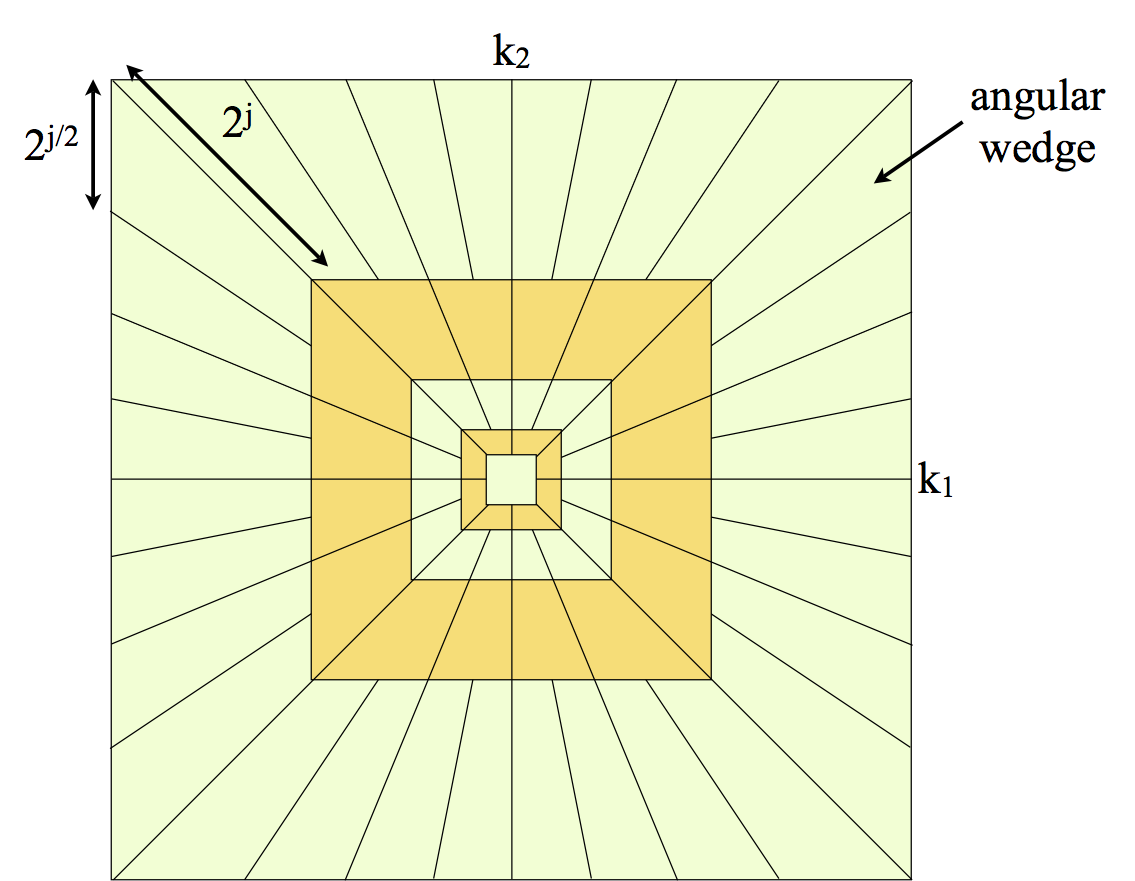
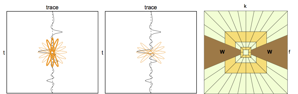
The curvelet transform naturally exploits the high-dimensional and strong geometrical structure of seismic data. The curvelet transform (Candès and Donoho, 2004) is designed to represent curve-like singularities optimally by decomposing seismic data into a superposition of localized plane waves, called curvelets. These curvelets are shaped according to a parabolic scaling law and have different frequency contents and dips to match locally the wavefront at best. See Figure 2 for a graphical depiction of this property.

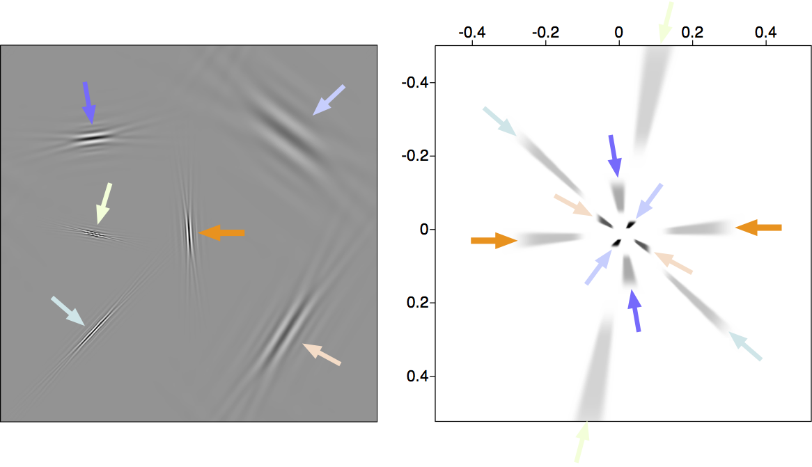
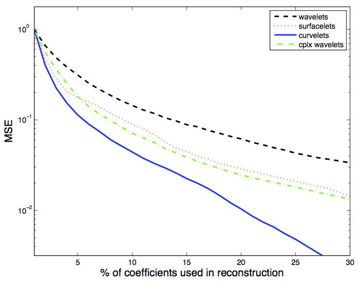
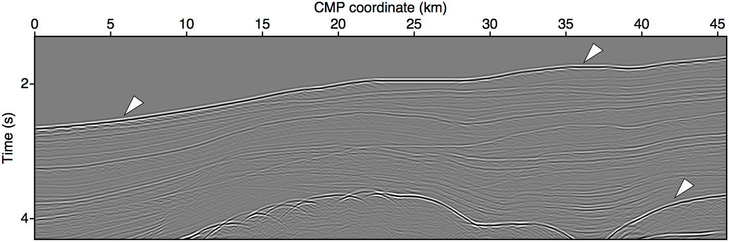
The scaling properties of these curvelets achieve the highest asymptotic order for coefficient sparsity¹ over all non-adaptive representations of regularly-sampled seismic data (see Figure 3). In other words, the superposition of only a “few” curvelets captures most of the energy of a seismic record.

The theoretical guarantees of curvelets are very general. Consequently, for any particular seismic dataset, it is usually possible to specifically construct even sparser representations by taking into account additional knowledge of the dataset, such sampling discretization choices, dominant frequencies, and acquisition geometry. For example, the Curvelet transform can be redefined on a non-uniform physical grid² (predetermined using knowledge of the actual acquisition coordinates) to emit sparse representations of irregularly sampled data.

Denoising

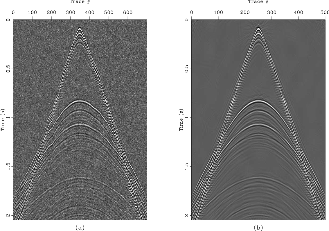
Given the assumption of additive noise, seismic denoising can be regarded as a simple model for the observed data: \[ \begin{equation*} \vec{d} = \vec{m} + \vec{n}, \end{equation*} \] where \(\vec{m}\) is the unknown noise-free seismic signal (what we call the “model”), and \(\vec{n}\) is a additive noise. In the Bayesian context, the prior assumptions on these two signals are crucial for a well-performing seismic denoising algorithm. Element-wise thresholding is a simple and useful technique to solve for \(\vec{m}\) if the model for \(\vec{n}\) is assumed to be a zero-centred Gaussian noise with standard deviation \(\sigma\), and \(\vec{m}\) is assumed to be sparse (following some “heavy-tailed” prior distribution).

Denoising via soft-thresholding

For seismic signals, \(\vec{m}\) will typically only be sparse under some transform. In this case, we can form an estimate of the model \(\est{\vec{m}}\) using the following simple, one-pass soft thresholding procedure (Hennenfent and Herrmann, 2006; Hennenfent, 2008): \[ \begin{equation} \est{\vec{m}} = \vec{S}^\dagger\mathrm{SoftTh\sigma}(\vec{S}\vec{d}). \label{denoise_softth} \end{equation} \] Operator \(\vec{S}\) is the forward transform which gives the coefficients of the signal in a sparsifying representation (along with its pseudoinverse \(\vec{S}^\dagger\) which returns coefficients to the physical space). For curvelet denoising, \(\vec{S}\) is the forward curvelet transform implemented with the Fast Discrete Curvelet Transform (FDCT, Candès et al., 2006), while \(\vec{S}^\dagger\) is the “inverse” curvelet transform³. The function \(\mathrm{SoftTh_\sigma}\) is a non-linear soft-thresholding applied element-wise on the transform domain coefficients according to: \[ \begin{equation} \mathrm{SoftTh_\sigma(x)} := \begin{cases} x - \mathrm{sign}(x)3\sigma & |x| \ge 3\sigma \\ 0 & |x| < 3\sigma. \end{cases} \label{softth} \end{equation} \] This thresholding scheme forms the maximum a-posteriori (MAP) estimator for a model signal given an additive Gaussian noise with standard deviation \(\sigma\) (Mallat, 1999). Its denoising efficacy is directly related to the ability of the transform domain \(\vec{S}\) to represent the desired signal sparsely while preserving the “Gaussian-ness” of noise.

Denoising via hybrid support identification and projections

One major shortcoming of the soft-thresholding approach is the loss of accurate amplitude information. The operation as shown in \(\eqref{softth}\) affects the amplitude of all coefficients in a uniform way, leading to a well-known “biasing” problem where smaller coefficients are less accurately reconstructed compared to larger ones. In turn, this effect can sometimes severely distort the amplitude of wavefronts, and often results in what are commonly known as “transform noise”. Since accurate amplitude information is usually considered critical in seismic applications, we can instead utilize a hybrid approach where we first identify the sparsest set of curvelets \(\Gamma\) that carry the majority of the signal, and then hard-threshold the rest of the coefficients.

When \(\vec{S}\) is not a unitary basis, such as the case with Curvelets, the coefficient support identification step can be done in an efficient manner by solving an \(\ell_1\)-minimization (often called “basis pursuit”) problem \[ \begin{equation} \min_\vec{x} \|\vec{x}\|_1\; \text{subject to}\; \|\vec{d} - \vec{S}^\dagger\vec{x}\|_2 \le \epsilon \label{denoise_bpdn} \end{equation} \] where \(\epsilon\) is some estimate of the 2-norm of the noise. This approach typically yields a sparser set of “significant” coefficients \(\Gamma\) compared to simply applying \(\vec{S}\) to \(\vec{d}\). Denoising is effectively achieved by projecting our data into this restricted set of significant coefficients (possibly after additional pruning of the coefficients from physical and statistical arguments). Algorithmically, this involves solving the system \[ \begin{equation*} \vec{d} = \vec{S}^T\vec{W}_\Gamma \est{\vec{x}} \end{equation*} \] in the least-squares sense (using, for example, CG-type methods) for \(\est{\vec{x}}\), where \(\vec{S}^T\) is the transpose of the curvelet transform operator, and \(\vec{W}_\Gamma\) a diagonal weighting matrix that is 1 if the corresponding column (representing one curvelet) of \(\vec{S}^T\) is part of the sparse set of curvelets that we identified to significantly represent our desired seismic signal via the basis pursuit problem \(\eqref{denoise_bpdn}\), and 0 otherwise. The final denoised data is then finally obtained by \(\est{\vec{m}} = \vec{S}^\dagger\est{\vec{x}}\).

Wavefield reconstruction

The problem of wavefield reconstruction (or interpolation) involves in-filling seismic data in areas where receivers or sources are not present. The missing data can be due to acquisition gaps, under-sampling of the source or receiver grid, or discarded dead traces. The most simplistic form of this problem assumes that the acquired traces can be neatly represented by a “mask” on the ideal acquisition grid, and is characterized by three pieces of information:

1. the actual acquired data
2. a “target” grid that reflects the desired acquisition geometry for our reconstructed wavefield
3. a mask \(\vec{R}\) that spatially locates the acquired traces within the target grid.

In this case we have the following model for our signal \[ \begin{equation*} \vec{d} = \vec{R}\vec{m}, \end{equation*} \] where the restriction matrix \(\vec{R}\) is constructed by taking the identity matrix \(\vec{I}\) and removing the rows that correspond to the missing data.

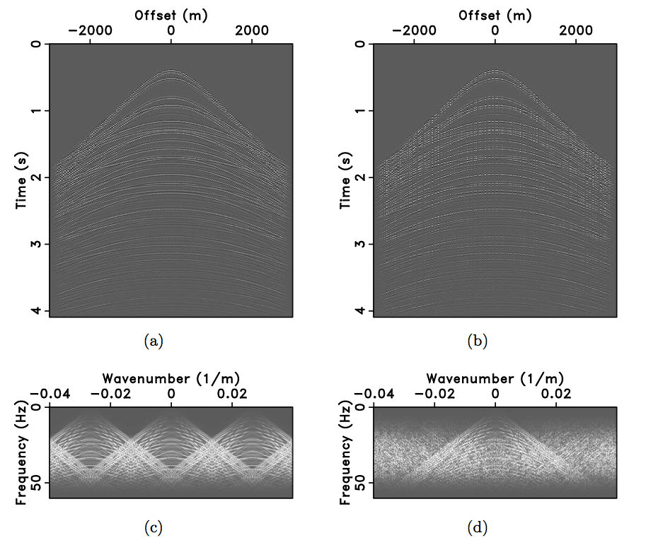
The manner in which the missing traces are located is a major factor in the properties the reconstruction problem. Specifically, it is known that randomness in the location of the missing traces creates favourable recovery problems. For example, uniform undersampling (i.e., regularly missing traces) creates coherent aliasing artifacts in the FK domain of the seismic data, but random undersampling instead leads to much more incoherent noise-like artifacts, which can be removed with methods similar to those described in the previous section. This property is studied in Hennenfent and Herrmann (2008), where a “jittered” undersampling technique is proposed as a acquisition geometry that both satisfies a coarse sampling (due to resource constraints) and creates favourable up-sampling properties by introducing controlled randomness in spatial coordinates.

Reconstruction via curvelet (co)sparsity

SLIM have published several papers proposing a wavefield reconstruction algorithm that is based on “denoising” incoherent FK noise induced by a random undersampling using curvelet sparsity (Herrmann and Hennenfent, 2008; Hennenfent and Herrmann, 2008). This method, called Curvelet Reconstruction with Sparsity-promoting Inversion (CRSI), attempts to find the sparsest set of curvelet coefficients that explain the acquired data by solving the basis pursuit problem \[ \begin{equation} \min_\vec{x} \|\vec{x}\|_1\; \text{subject to}\; \|\vec{d} - \vec{R}\vec{S}^\dagger\vec{x}\|_2 \le \epsilon \label{CRSI_bpdn} \end{equation} \] where the reconstructed wavefield is then given by applying \(\vec{S}^\dagger\) to the solution.

The behaviour of problem \(\eqref{CRSI_bpdn}\) using curvelets can be analyzed in in terms of compressive sensing theory under an overcomplete dictionary (Candes et al., 2006, 2011). One immediate result is that the measurement system (in our case \(\vec{R}\)) should be “maximally incoherent”⁴ with the reconstruction dictionary (in our case curvelets) in order to maximize the degree of undersampling that \(\eqref{CRSI_bpdn}\) can overcome. In other words, a successful reconstruction for any given degree of undersampling necessitates that we excludes curvelets that can sparsely represent missing traces.

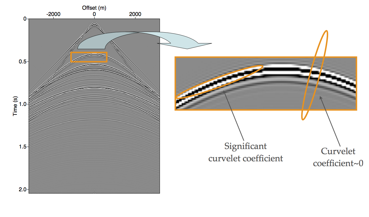
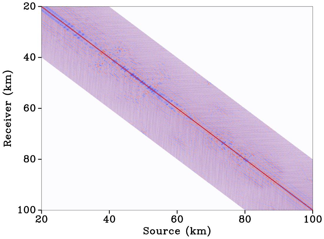
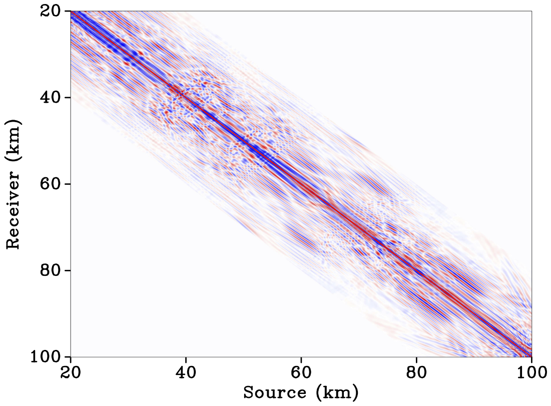
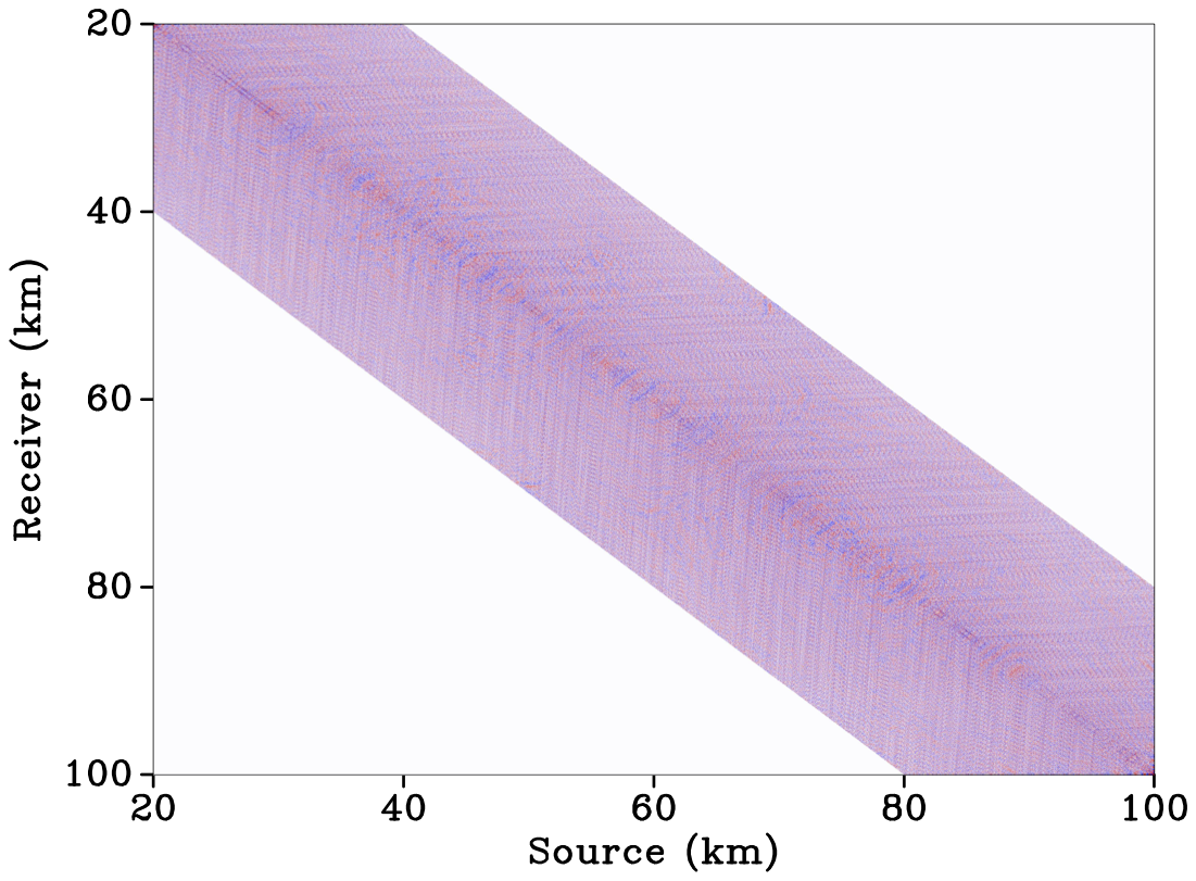
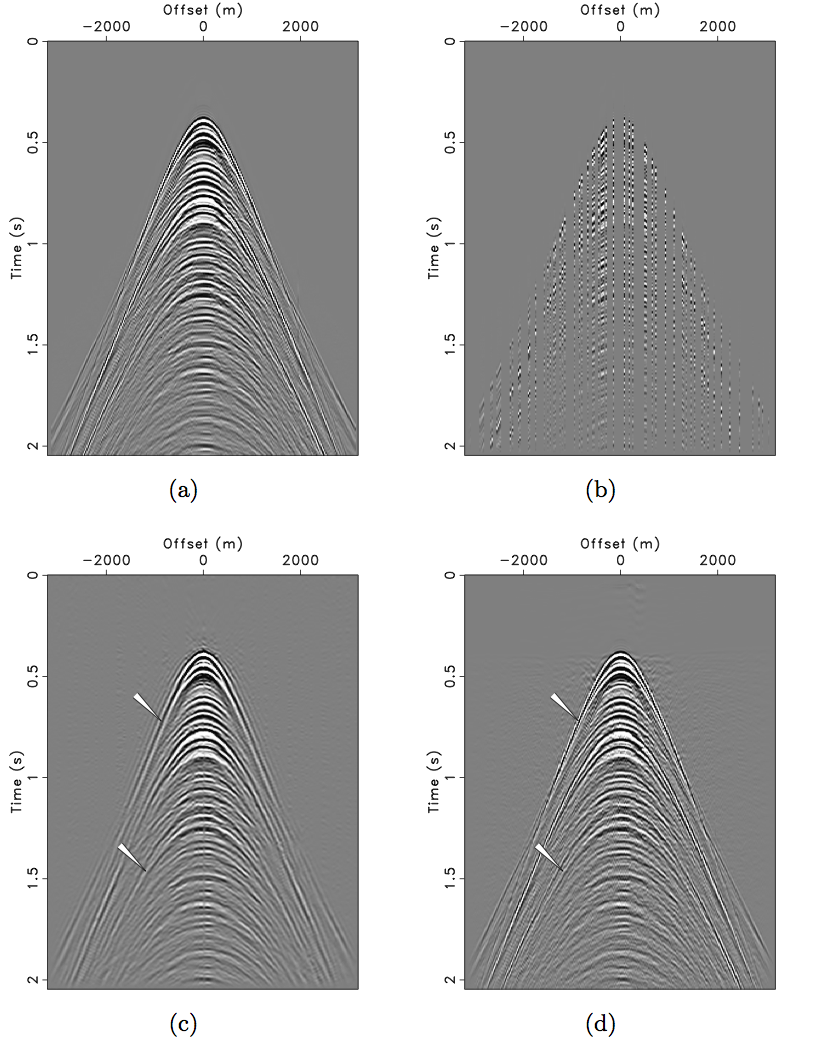
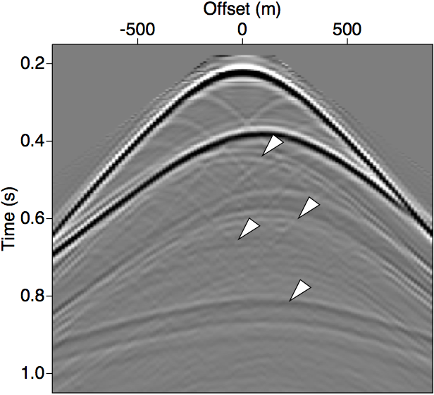
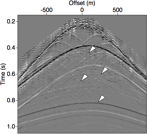
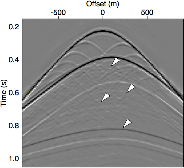
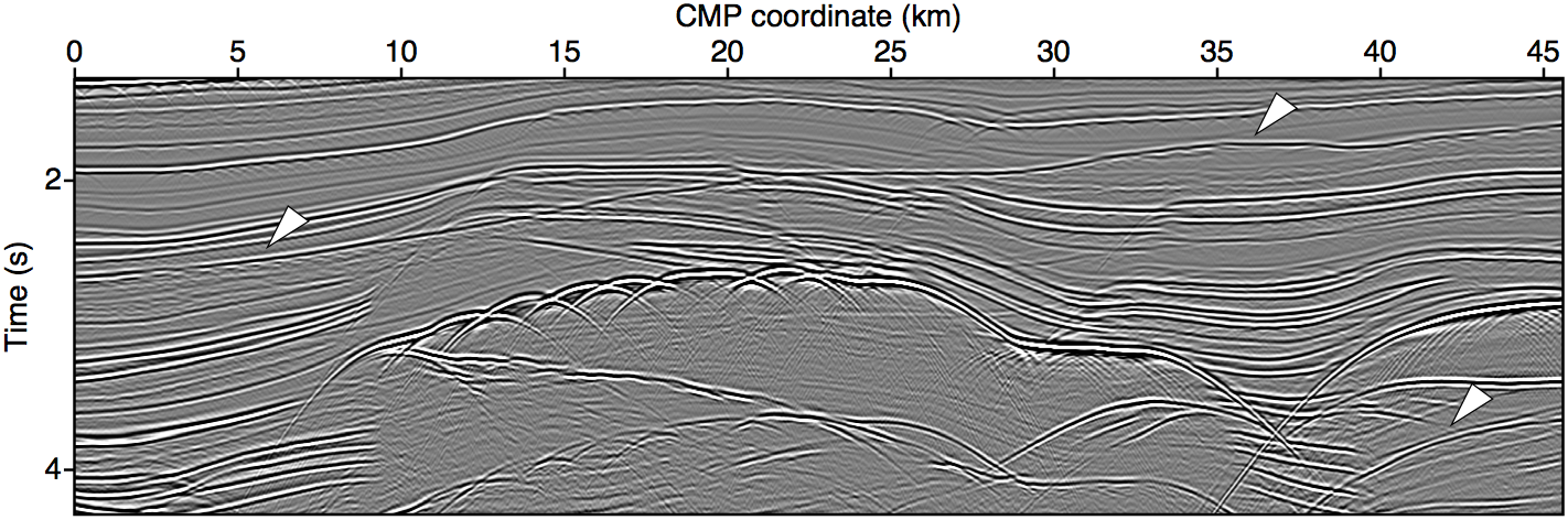
The above principle has an interesting consequence for seismic data reconstruction. Since the time-axis is usually fully sampled (as missing data is usually caused by missing source or receivers), we have an inherent anisotropy in the shape of the missing data artifact. As Figure 7 shows, vertically-oriented curvelets happen to sparsely represent an empty trace, as it is highly discontinuous in the spatial direction yet smooth (constant) in the temporal direction. To improve our recovery, CRSI typically employ an annular weighting of the curvelet coefficients to mask out these vertically-oriented curvelets. In the end, this translates into solving problem \(\eqref{CRSI_bpdn}\) using the modified curvelet frame \(\vec{S}_\theta := \vec{W}_\theta\vec{S}\) instead of \(\vec{S}\), where \(\vec{W}_\theta\) is a diagonal matrix that is 0 when the corresponding row of \(\vec{S}\) represents a vertically-oriented curvelet, and 1 elsewhere. This method is typically called “Focused CRSI”. See Figure 8 for a seismic datacube reconstruction example from real data.

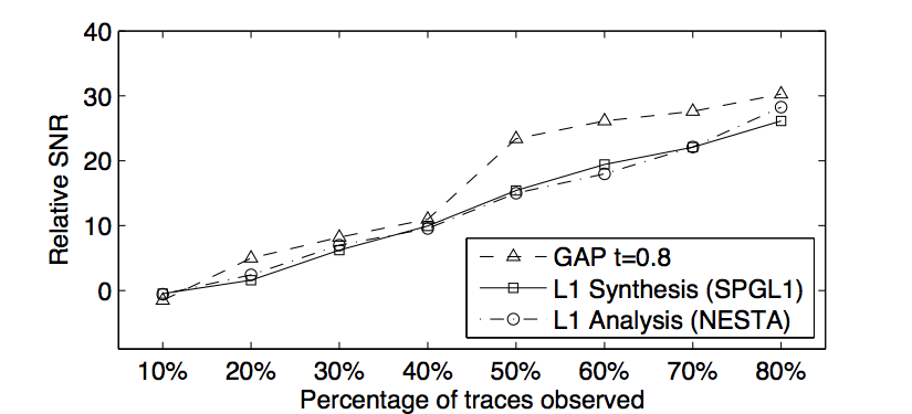
Some recent results in signal reconstruction from frames described a possible benefit in investigating an alternative form of the problem (Elad et al., 2007; Nam2013; Lin and Herrmann, 2013b) called the “analysis” formulation. Compared to the above CRSI example, the analysis problem is written as \[ \begin{equation} \min_\vec{m} \|\vec{S}\vec{m}\|_1\; \text{subject to}\; \|\vec{d} - \vec{R}\vec{m}\|_2 \le \epsilon. \label{CRSI_analy} \end{equation} \] Note that, if \(\vec{S}\) is a unitary basis, then both \(\eqref{CRSI_bpdn}\) and \(\eqref{CRSI_analy}\) will give identical solutions. However, in the case where \(\vec{S}\) is an overcomplete dictionary like curvelets, the analysis form \(\eqref{CRSI_analy}\) is akin to further imposing the constraint \(\vec{x} = \vec{S}\vec{S}^\dagger\vec{x}\) on solutions of \(\eqref{CRSI_bpdn}\), leading to a stronger regularizer compared to the standard CRSI.

As discussed in Lin and Herrmann (2013b), solving the problem \(\eqref{CRSI_analy}\) as-is does not lead to appreciably different solutions compared to the original problem \(\eqref{CRSI_bpdn}\), when the same solver is used. However, a recently proposed method called Greedy Analysis Pursuit (GAP, Nam et al., 2011, 2013) is found to be able to uniformly improve the reconstruction solutions of \(\eqref{CRSI_analy}\) by aggressively identifying the set of curvelets that are not supporting the signal, and forcing the solutions to be orthogonal to this set of curvelets. The success of this method fundamentally relies on a new concept called “cosparsity” which can be seen as the theoretical analogue of “sparsity” for the set of curvelets that do support the signal.

Reconstruction via low-rank matrix or tensor completion

In addition to relying on curvelet sparsity to remove undersampling artifacts, seismic data reconstruction can instead exploit low-rank properties of the seismic wavefield datacube for reconstruction. This approach can be seen as an application of matrix/tensor completion in applied mathematics. In this case, we seek the lowest-rank model signal that explains our observed traces. Since this approach does not involve the curvelet transform, it can be significantly faster and more memory efficient. See Matrix completion under Structure-promoting optimization.

Robust estimation of primaries by \(\ell_1\)-regularized inversion

The basic assumption of surface-related multiple removal with EPSI is that, with noiseless and perfectly sampled up-going seismic wavefield \(\vec{P}\) at the Earth’s surface (with seismic reflectivity operator \(\vec{R}\), typically close to \(\vec{-I}\)) due to a finite energy source wavefield \(\vec{Q}\), there exists an operator \(\vec{G}\) for every frequency in the seismic bandwidth such that the relation \[ \begin{equation*} \vec{P} = \vec{G}\vec{Q} + \vec{R}\vec{G}\vec{P} \end{equation*} \] holds true. Here we use the “detail-hiding” notation (Berkhout and Pao, 1982) where all upper-case bold quantities are monochromatic data-matrices, with the row index corresponding to the discretized receiver positions and column index the source positions. Moreover, \(\vec{G}\) is interpreted as the (surface) multiple-free subsurface Green’s function. The term \(\vec{GQ}\) is interpreted as the primary wavefield, while the term \(\vec{R}\vec{G}\vec{P}\) contains all surface-related multiples.

Since only \(\vec{P}\) can be measured, inverting the above relation for \(\vec{GQ}\) admits non-unique solutions without additional regularization. Based on the argument that a discretized physical representation of \(\vec{G}\) resemble a wavefield with impulsive wavefronts, the Robust EPSI algorithm (REPSI, Lin and Herrmann, 2013a) attempts to find the sparsest possible \(\vec{g}\) in the physical domain (from here on, all lower-case symbols indicate discretized physical representations of previously defined quantities). Specifically, it solves the following optimization problem in the space-time domain: \[ \begin{gather} \label{eq:EPSIopt} \min_{\vector{g},\;\vector{q}}\|\vector{g}\|_1 \quad\text{subject to}\quad f(\vec{g},\vec{q};\vec{p}) \le \sigma,\\ \nonumber f(\vec{g},\vec{q};\vec{p}) := \|\vector{p} - M(\vector{g},\vector{q};\vector{p})\|_2, \end{gather} \] where the forward-modeling function \(M\) can be written in terms of the data-matrix notation \(M(\vector{G},\vector{Q};\vector{P}) := \vec{G}\vec{Q} + \vec{R}\vec{G}\vec{P}\). Problem \(\eqref{eq:EPSIopt}\) essentially asks for the sparsest (via minimizing the \(\ell_1\)-norm) multiple-free impulse response that explains the surface multiples in \(\vector{p}\), while ignoring some amount of noise as determined by \(\sigma\).

The problem \(\eqref{eq:EPSIopt}\) is solved by a continuation scheme that involves alternatively solving two subproblems \[ \begin{align} \label{EPSI_fixG} \vector{g}_{k+1} &= \argmin_\vector{g}\|\vector{p} - \vector{M}_{q_k} \vector{g}\|_2\;\text{subject to}\;\|\vector{g}\|_1 \le \tau_k\\ \label{EPSI_fixQ} \vector{q}_{k+1} &= \argmin_\vector{q}\|\vector{p} - \vector{M}_{g_{k+1}} \vector{q}\|_2. \end{align} \] When \(\tau_k\) is small, solutions to the \(\ell_1\) constrained problem \(\eqref{EPSI_fixG}\) tends to be sparse and temporally impulsive, which well-approximates a full-band Green’s function. Therefore, approximation of the wavelet with \(\eqref{EPSI_fixQ}\) becomes a simple matter of matching the spectrally full-band \(\vector{g}_{k+1}\) to the spectral shape of our data. We choose \(\tau_k\) by gradually letting it grow \(\tau_{k+1} > \tau_k\) according to the pareto curve of the \(\ell_1\)-regularized misfit minimization problem (Hennenfent et al., 2008; van den Berg and Friedlander, 2008; Lin and Herrmann, 2013a) until we find the smallest \(\tau\) (and hence smallest \(\ell_1\) norm of \(\vector{g}\)) that gives our target misfit for the original REPSI problem \(\eqref{eq:EPSIopt}\).

References

Berkhout, A. J., and Pao, Y. H., 1982, Seismic Migration - Imaging of Acoustic Energy by Wave Field Extrapolation: Journal of Applied Mechanics, 49, 682. doi:10.1115/1.3162563
Candes, E. J., Eldar, Y. C., Needell, D., and Randall, P., 2011, Compressed sensing with coherent and redundant dictionaries: Applied and Computational Harmonic Analysis, 31, 59–73. doi:10.1016/j.acha.2010.10.002
Candes, E. J., Romberg, J., and Tao, T., 2006, Stable signal recovery from incomplete and inaccurate measurements: Communications on Pure and Applied Mathematics, 59, 1207.
Candès, E. J., and Donoho, D. L., 2004, New tight frames of curvelets and optimal representations of objects with \({C}^{2}\) singularities: Communications on Pure and Applied Mathematics, 57, 219–266.
Candès, E. J., Demanet, L., Donoho, D. L., and Ying, L., 2006, Fast discrete curvelet transforms (FDCT): Multiscale Modeling and Simulation, 5, 861–899.
Elad, M., Milanfar, P., and Rubinstein, R., 2007, Analysis versus synthesis in signal priors: Inverse Problems, 23, 947–968. doi:10.1088/0266-5611/23/3/007
Hennenfent, G., 2008, Sampling and reconstruction of seismic wavefields in the curvelet domain: PhD thesis,. The University of British Columbia. Retrieved from https://slim.gatech.edu/Publications/Public/Thesis/2008/hennenfent08phd.pdf
Hennenfent, G., and Herrmann, F. J., 2006, Seismic denoising with nonuniformly sampled curvelets: Computing in Science & Engineering, 8, 16–25. doi:10.1109/MCSE.2006.49
Hennenfent, G., and Herrmann, F. J., 2008, Simply denoise: Wavefield reconstruction via jittered undersampling: Geophysics, 73, V19–V28. doi:10.1190/1.2841038
Hennenfent, G., van den Berg, E., Friedlander, M. P., and Herrmann, F. J., 2008, New insights into one-norm solvers from the Pareto curve: Geophysics, 73, A23–A26. doi:10.1190/1.2944169
Herrmann, F. J., and Hennenfent, G., 2008, Non-parametric seismic data recovery with curvelet frames: Geophysical Journal International, 173, 233–248. doi:10.1111/j.1365-246X.2007.03698.x
Herrmann, F. J., Wang, D., and Verschuur, D. J., 2008a, Adaptive curvelet-domain primary-multiple separation: Geophysics, 73, A17–A21. doi:10.1190/1.2904986
Herrmann, F. J., Wang, D., Hennenfent, G., and Moghaddam, P. P., 2008b, Curvelet-based seismic data processing: A multiscale and nonlinear approach: Geophysics, 73, A1–A5. doi:10.1190/1.2799517
Kumar, V., 2009, Incoherent noise suppression and deconvolution using curvelet-domain sparsity: Master’s thesis,. The University of British Columbia. Retrieved from https://slim.gatech.edu/Publications/Public/Thesis/2009/kumar09THins.pdf
Lin, T. T., and Herrmann, F. J., 2013a, Robust estimation of primaries by sparse inversion via one-norm minimization: Geophysics, 78, R133–R150. doi:10.1190/geo2012-0097.1
Lin, T. T., and Herrmann, F. J., 2013b, Cosparse seismic data interpolation: EAGE annual conference proceedings. doi:10.3997/2214-4609.20130387
Mallat, S., 1999, A wavelet tour of signal processing, second edition: Academic Press.
Nam, S., Davies, M., Elad, M., and Gribonval, R., 2011, Recovery of cosparse signals with greedy analysis pursuit in the presence of noise: In CAMSAP - 4th international workshop on computational advances in multi-sensor adaptive processing - 2011. Retrieved from http://hal.inria.fr/hal-00691162
Nam, S., Davies, M., Elad, M., and Gribonval, R., 2013, The cosparse analysis model and algorithms: Applied and Computational Harmonic Analysis, 34, 30–56. doi:10.1016/j.acha.2012.03.006
van den Berg, E., and Friedlander, M. P., 2008, Probing the Pareto frontier for basis pursuit solutions: SIAM Journal on Scientific Computing, 31, 890–912. doi:10.1137/080714488
Wang, D., Saab, R., Yilmaz, O., and Herrmann, F. J., 2008, Bayesian wavefield separation by transform-domain sparsity promotion: Geophysics, 73, 1–6. doi:10.1190/1.2952571
Yarham, C., and Herrmann, F. J., 2008, Bayesian ground‐roll separation by curvelet‐domain sparsity promotion: In SEG technical program expanded abstracts 2008 (pp. 2576–2580). doi:10.1190/1.3063878
Technically, this is measured by the sorted coefficient amplitude decay expressed as the order of a asymptotic power law. Theory dictates that curvelets achieve the fastest possible decaying order for non-adaptive frames.↩
Via the nonqeuispaced Fourier transform.↩
Because curvelet are defined as tight frames, the pseudoinverse of \(\vec{S}\) is actually its transpose, analogous to the cases where \(\vec{S}\) is a unitary basis.↩
Technically, expressed as the maximum inner product between any pair of columns of \(\vec{R}\) and \(\vec{S}\); the smaller this maximum value is the better we can expect our reconstruction to be.↩