Uncertainty quantification

Seismic imaging and uncertainty quantification

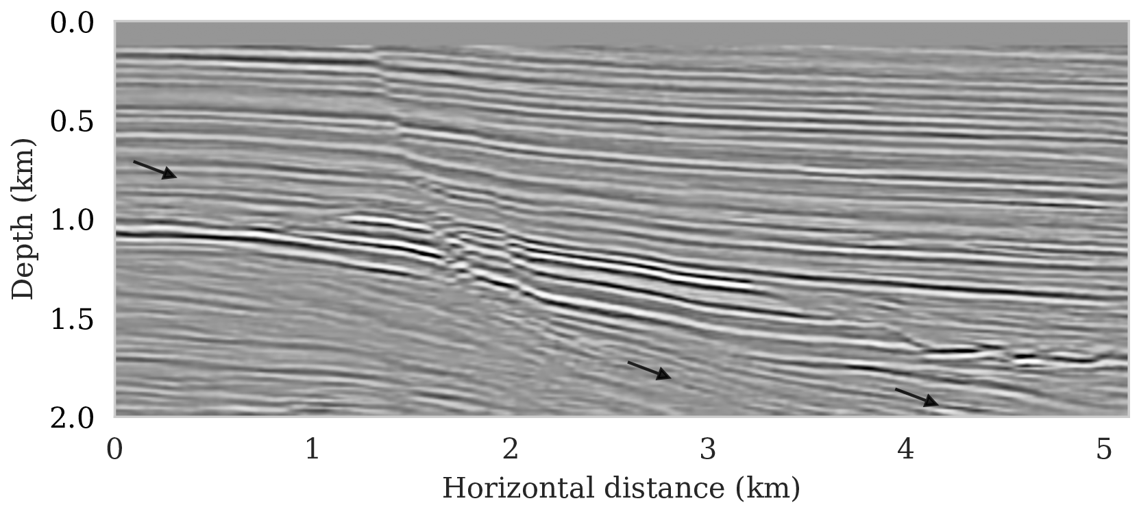
Seismic imaging deals with extracting physical properties of the subsurface, e.g., the seismic velocity and density, from large volumes of measurements that are recorded at the Earth’s surface (Yilmaz, 2001). The wave equation represents the underlying physical data generation phenomena, linking the mentioned media properties of the Earth subsurface to observed data.

Deep Bayesian inference for seismic imaging with tasks

(Published in Siahkoohi et al. (2022) with software available here)

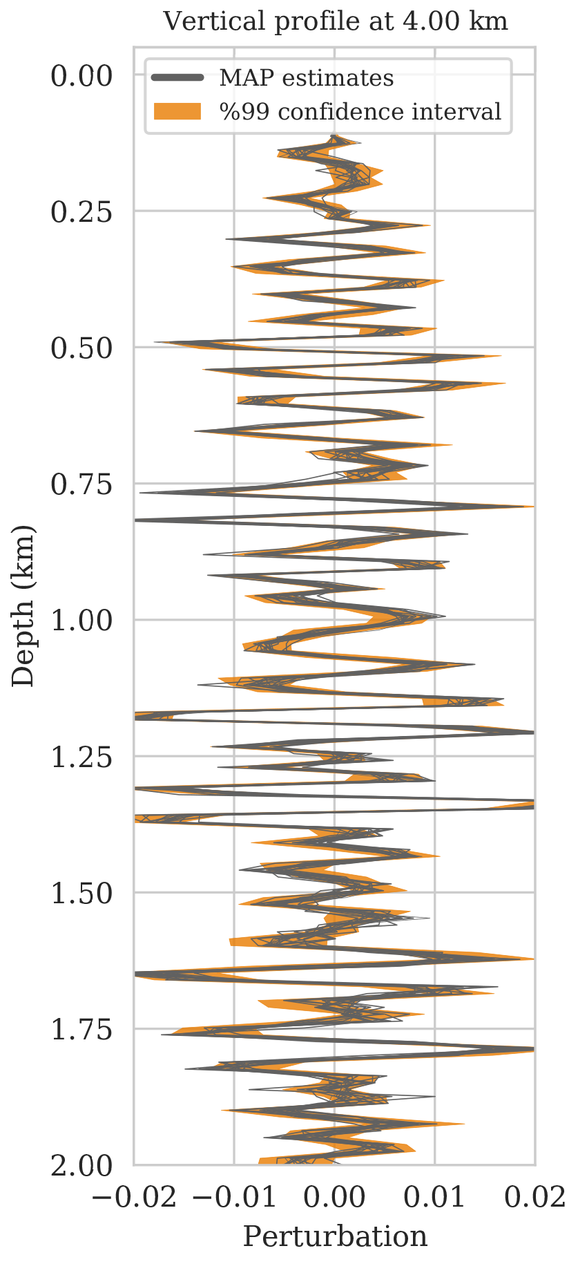
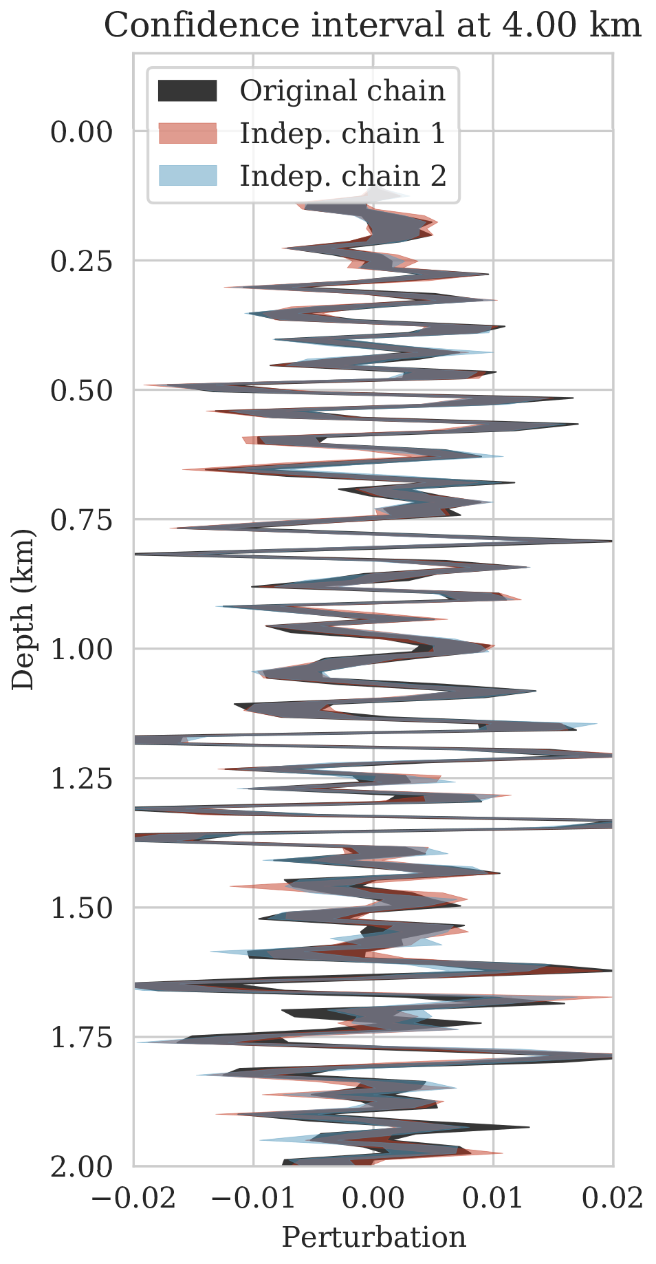
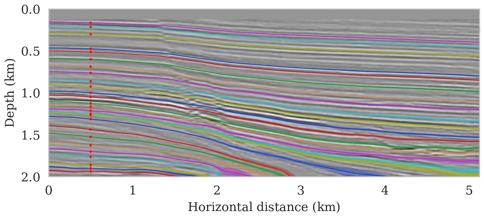
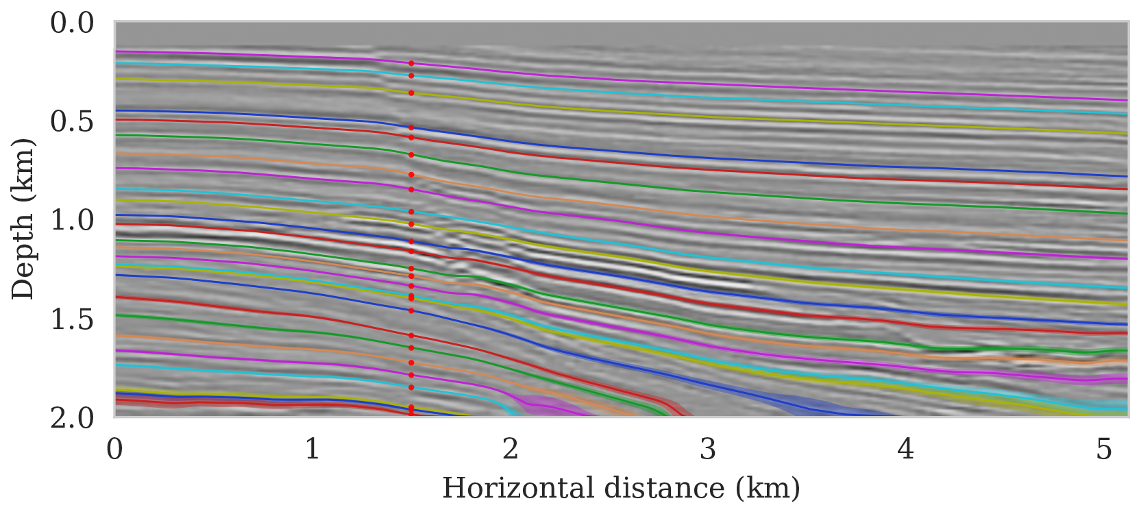
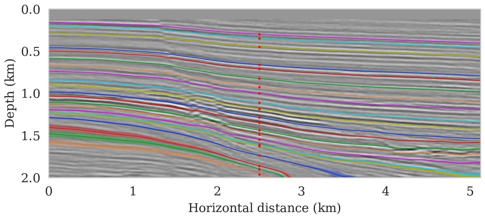
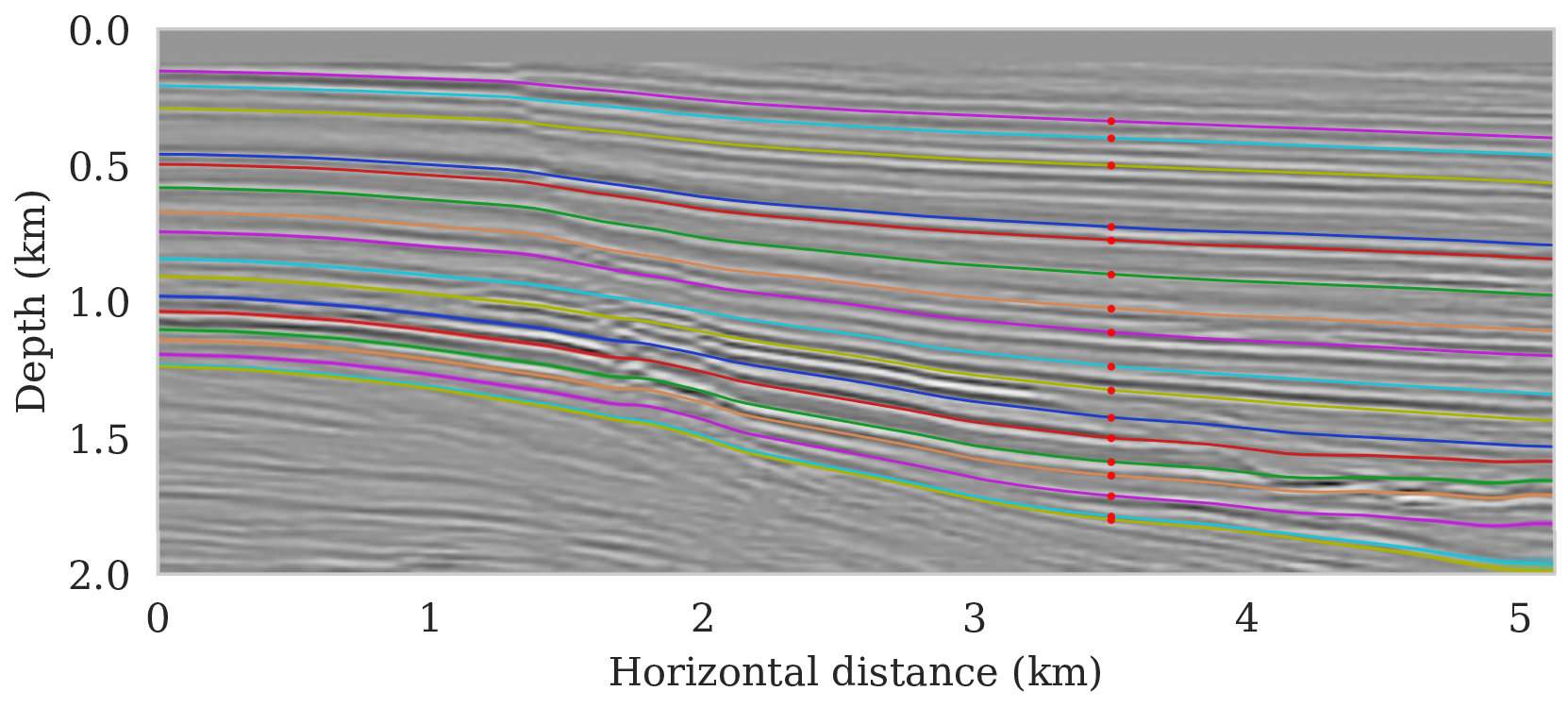
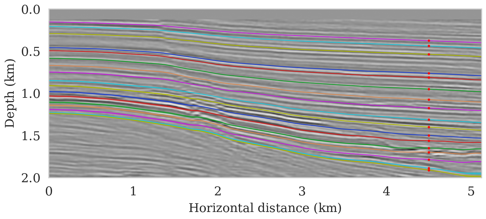
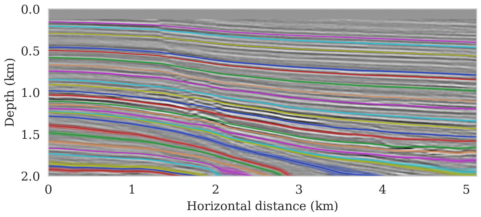
We propose to use techniques from Bayesian inference and deep neural networks to translate uncertainty in seismic imaging to uncertainty in tasks performed on the image, such as horizon tracking. Seismic imaging is an ill-posed inverse problem because of bandwidth and aperture limitations, which is hampered by the presence of noise and linearization errors. Many regularization methods, such as transform-domain sparsity promotion, have been designed to deal with the adverse effects of these errors, however, these methods run the risk of biasing the solution and do not provide information on uncertainty in the image space and how this uncertainty impacts certain tasks on the image. A systematic approach is proposed to translate uncertainty due to noise in the data to confidence intervals of automatically tracked horizons in the image. The uncertainty is characterized by a convolutional neural network (CNN) and to assess these uncertainties, samples are drawn from the posterior distribution of the CNN weights, used to parameterize the image. Compared to traditional priors, it is argued in the literature that these CNNs introduce a flexible inductive bias that is a surprisingly good fit for a diverse set of problems, including medical imaging, compressive sensing, and diffraction tomography. The method of stochastic gradient Langevin dynamics is employed to sample from the posterior distribution. This method is designed to handle large scale Bayesian inference problems with computationally expensive forward operators as in seismic imaging. Aside from offering a robust alternative to maximum a posteriori estimate that is prone to overfitting, access to these samples allow us to translate uncertainty in the image, due to noise in the data, to uncertainty on the tracked horizons. For instance, it admits estimates for the pointwise standard deviation on the image and for confidence intervals on its automatically tracked horizons. \[ \begin{equation} \begin{aligned} & \B{w}_{k+1} = \B{w}_{k} - \frac{\alpha_k}{2} \B{M}_k \nabla_{\B{w}} \left ( \frac{n_s }{2 \sigma^2} \big \| \B{d}_i- \B{J}(\B{m}_0, \B{q}_i) {g} (\B{z}, \B{w}_k) \big \|_2^2 + \frac{\lambda^2}{2} \big \| \B{w}_k \big \|_2^2 \right ) + \boldsymbol{\eta}_k, \\ & \boldsymbol{\eta}_k \sim \mathrm{N}( \B{0}, \alpha_k \B{M}_k), \end{aligned} \label{sgld} \end{equation} \] Below we apply this method to seismic imaging.

\[ \begin{equation} \begin{aligned} \mathbb{E}_{\B{h} \sim p_{\text{post}} \left (\B{h} \mid \B{d} \right )} \ \left [ f \left (\B{h} \right) \right ] & = \int f \left ( \B{h} \right) p_{\text{post}} \left (\B{h} \mid \B{d} \right ) \mathrm{d} \B{h} = \iint f \left (\B{h} \right) p \left (\B{h}, \delta \B{m} \mid \B{d} \right ) \mathrm{d} \B{h}\, \mathrm{d} \delta \B{m} \\ & = \iint f \left (\B{h} \right) p_{\mathcal{H}} \left (\B{h} \mid \delta \B{m}, \B{d} \right ) p_{\text{post}} \left ( \delta \B{m} \mid \B{d} \right ) \mathrm{d} \B{h}\, \mathrm{d} \delta \B{m} \\ & = \iint f \left (\B{h} \right) p_{\mathcal{H}} \left (\B{h} \mid \delta \B{m} \right ) p_{\text{post}} \left ( \delta \B{m} \mid \B{d} \right ) \mathrm{d} \B{h}\, \mathrm{d} \delta \B{m} \\ & = \mathbb{E}_{\delta \B{m} \sim p_{\text{post}} \left (\delta \B{m} \mid \B{d} \right ) } \left [ \int f \left (\B{h} \right) p_{\mathcal{H}} \left (\B{h} \mid \delta \B{m} \right ) \mathrm{d} \B{h} \right ] \\ & = \underbrace {\mathbb{E}_{\delta \B{m} \sim p_{\text{post}} \left (\delta \B{m} \mid \B{d} \right ) } \underbrace {\mathbb{E}_{ \B{h} \sim p_{\mathcal{H}} \left (\B{h} \mid \delta \B{m} \right ) } \left [ f \left (\B{h} \right) \right ]. }_{\substack{ \text{ uncertainty in} \\ \text{ horizon tracking}}}}_{ \substack{\text{ uncertainty in} \text{ seismic imaging}}} \\ \end{aligned} \label{horizon-inference} \end{equation} \]

Bayesian inference on high-dimensional inverse problems with computationally expensive forward modeling operators, has been, and continues to be a major challenge in the field of seismic imaging. Aside from obvious computational challenges, the selection of effective priors is problematic given the heterogeneity across geological scenarios and scales exhibited by elastic properties of the Earth’s subsurface. To limit the possibly heavy-handed bias induced by a handcrafted prior, we propose regularization via deep priors. During this type of regularization, seismic images are restricted to the range of an untrained convolutional neural network with a fixed input, randomly initialized. Compared to conventional regularization, which tends to bias solutions towards sometimes restrictive choices made in defining these prior distributions, nonlinear deep priors derive regularizing properties from their overparameterized network architecture. The reparameterization of the seismic image by means of a deep prior leads to a Bayesian formulation where the prior is a Gaussian distribution of the weights of the network.

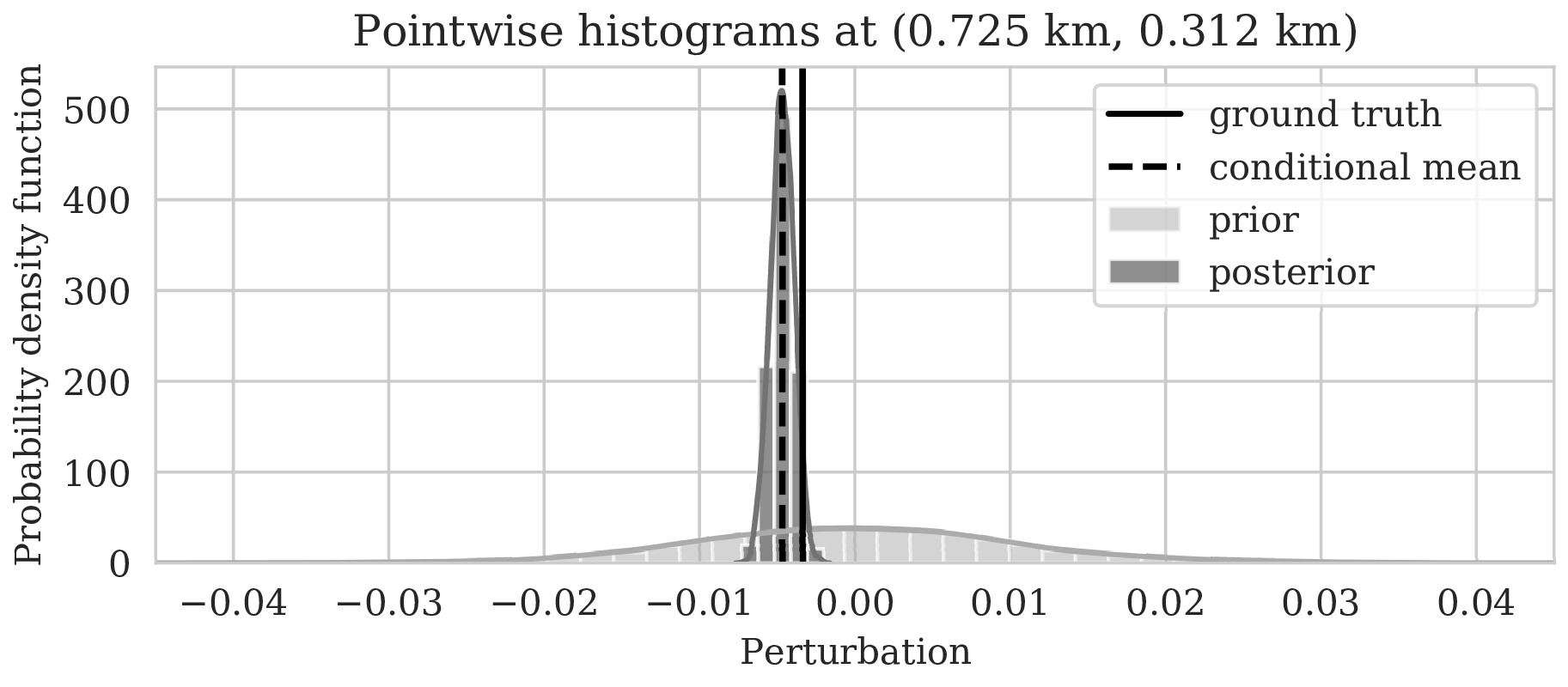
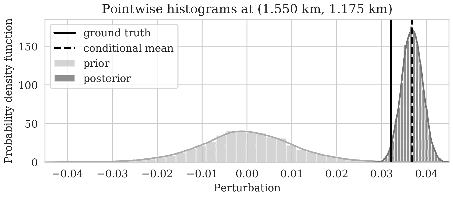
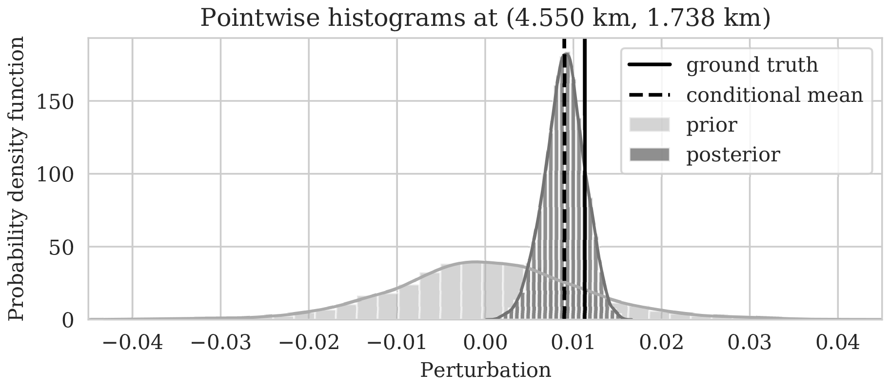
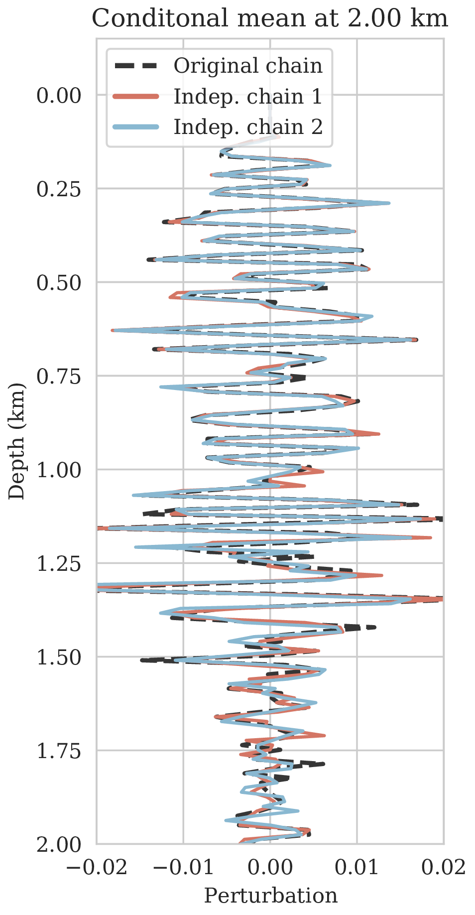
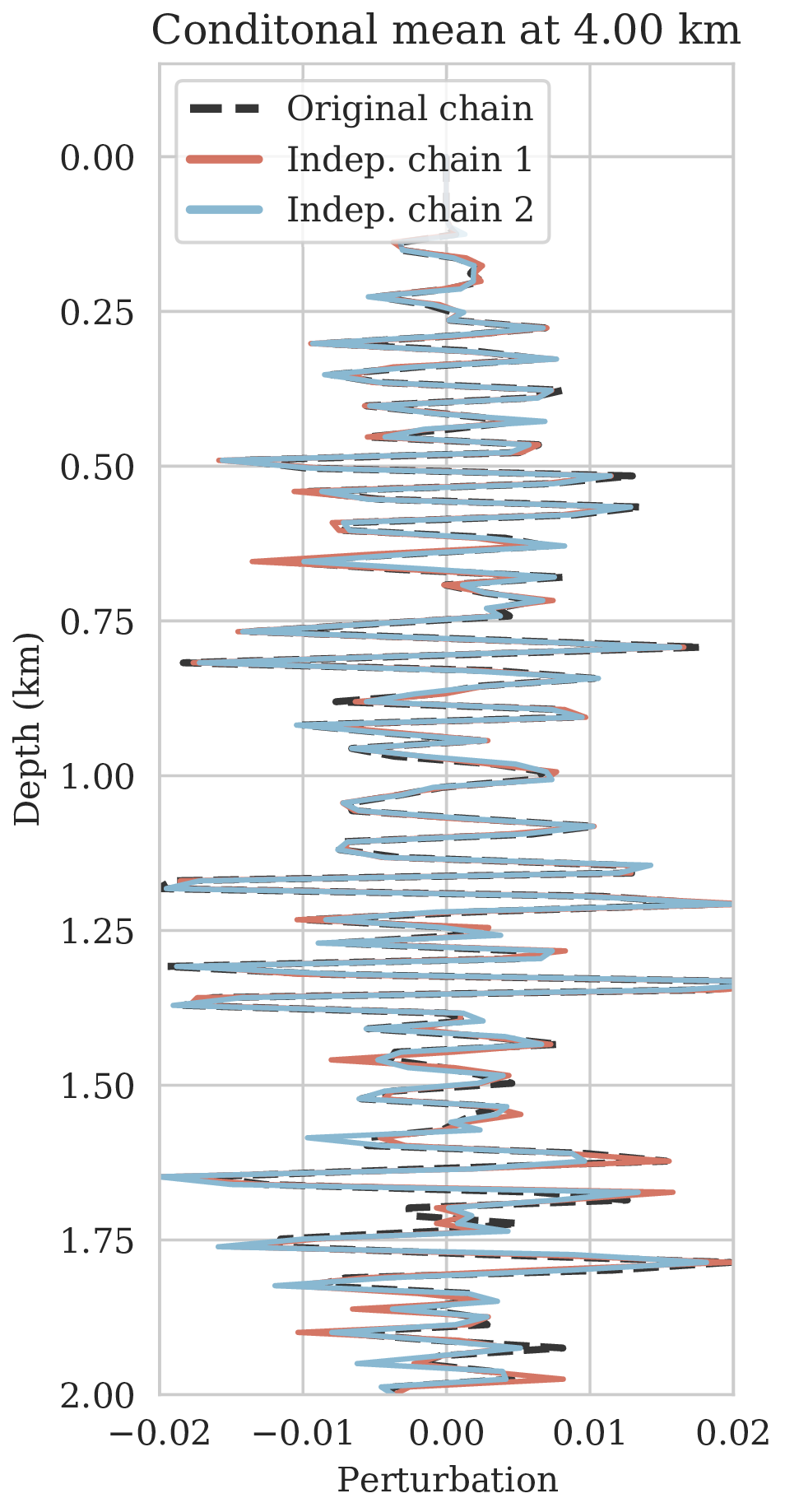
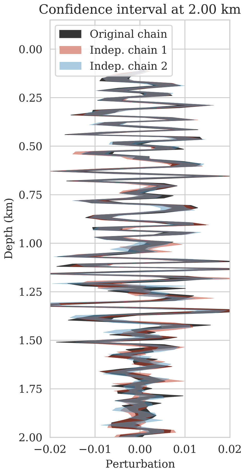
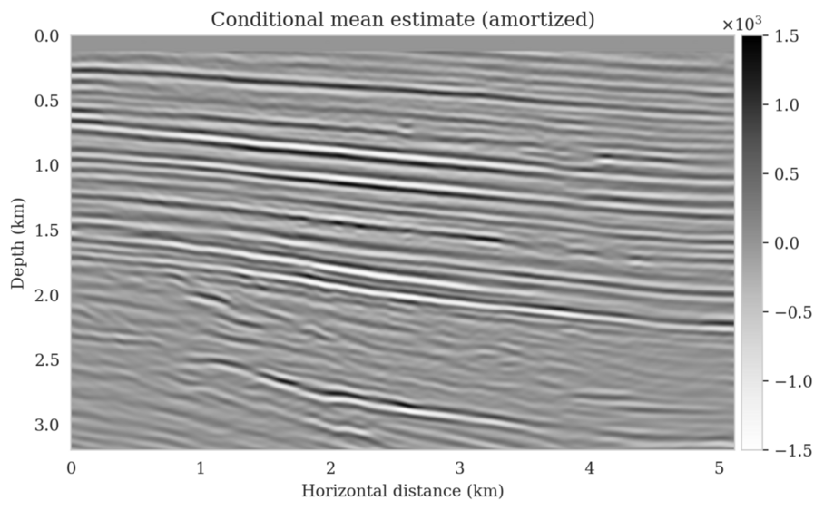
As long as overfitting can be avoided, regularization with deep priors is known to produce perceptually accurate results, an observation we confirmed in the context of controlled seismic imaging experiments. Unfortunately, preventing fitting the noise is difficult in practice. In addition, there is always the question how errors, e.g., bandwidth-limited noise or linearization errors, propagate to uncertainty in the image and to certain tasks to be carried out on the image, which for instance includes the task of automatic horizon tracking. To answer this question and to avoid the issue of overfitting, we propose to sample from the imaging posterior distribution and use the samples to compute the conditional mean estimate, which in our experiments exhibited more robustness to noise, and to obtain confidence intervals for the tracked horizons via our probabilistic horizon tracking framework.

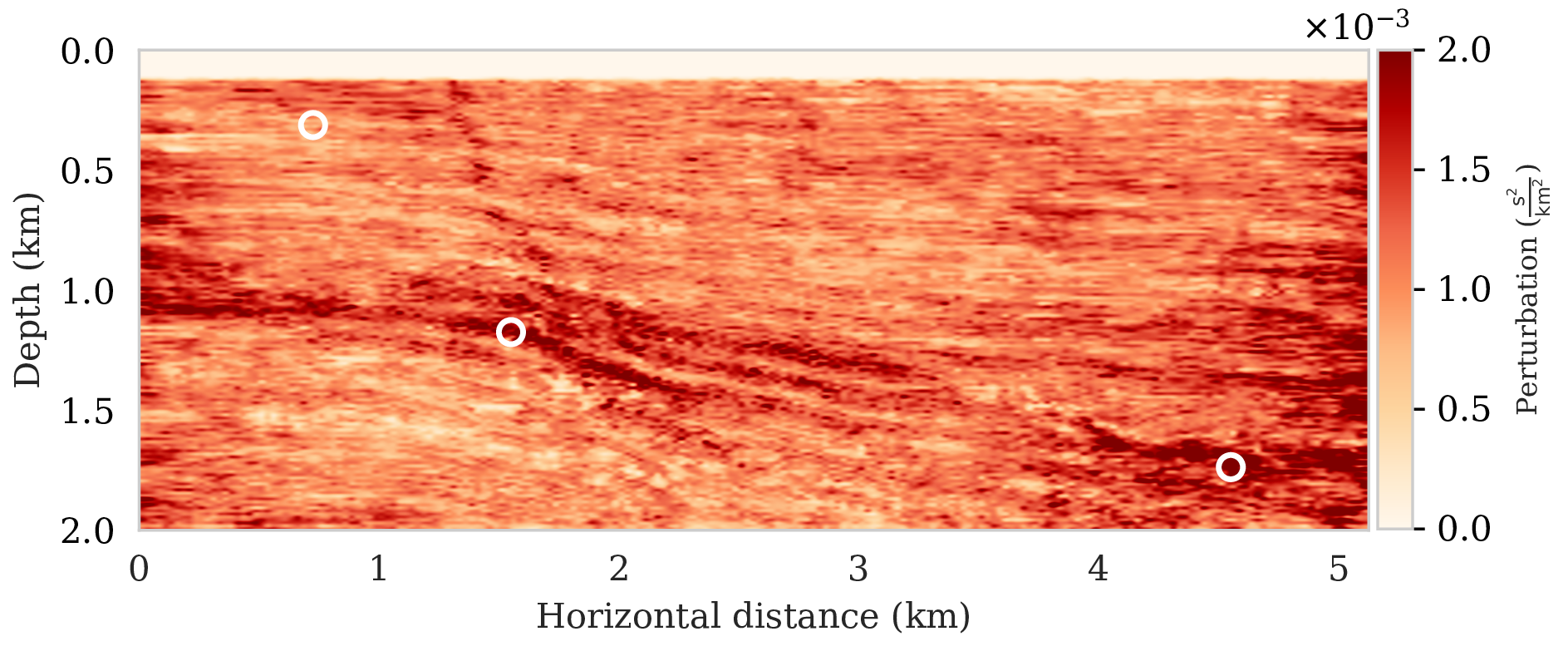
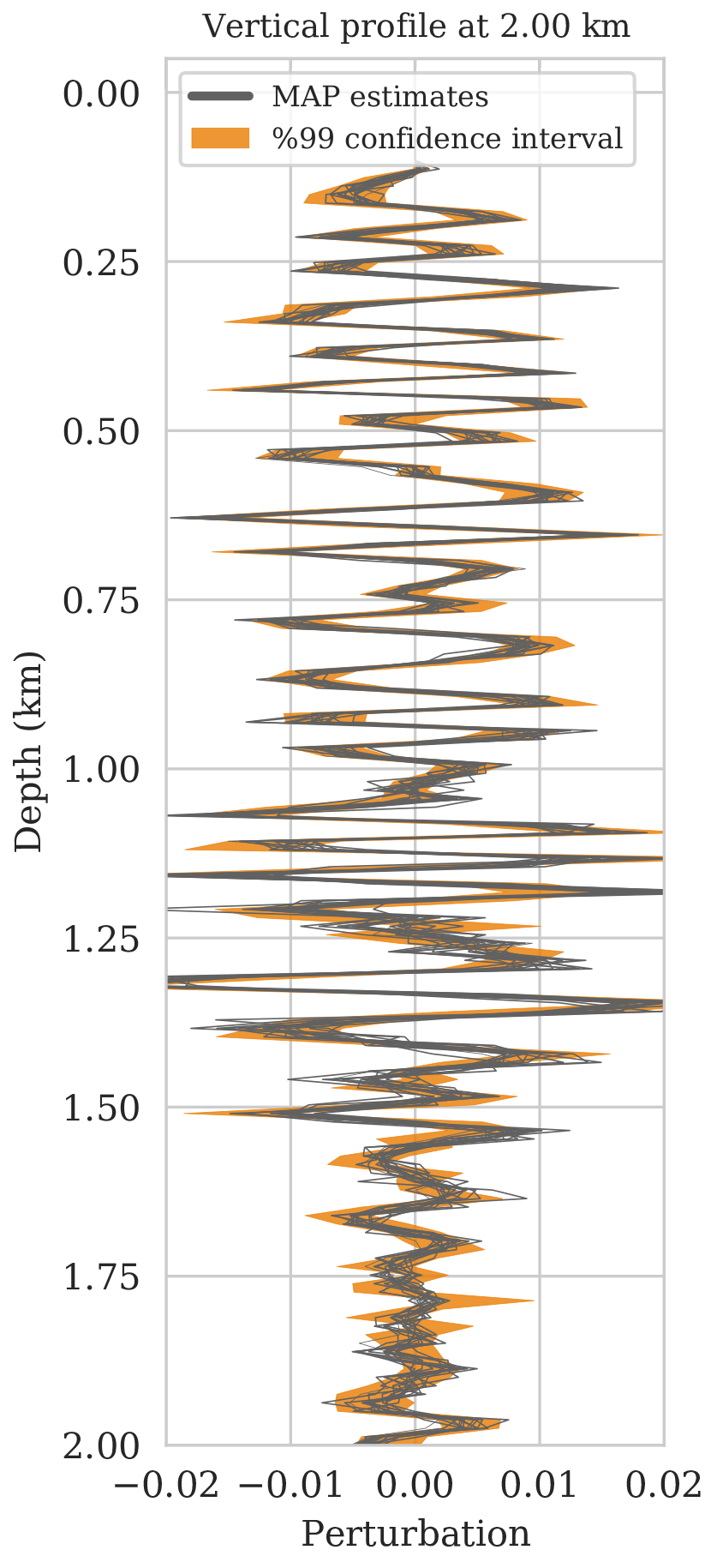
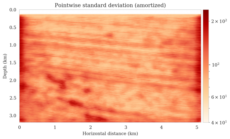
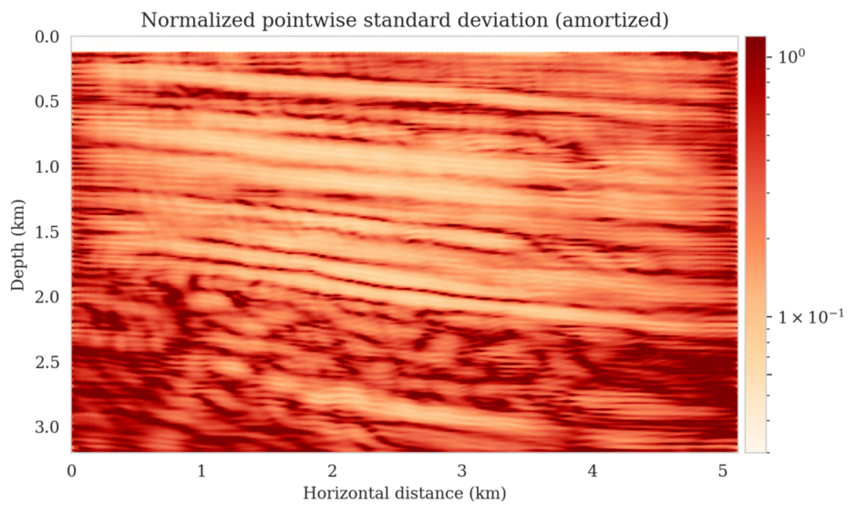
Even though drawing samples from the posterior is computationally burdensome, it allows us to mitigate the imprint of overfitting while it is also conducive to a systematic framework mapping errors in shot data to uncertainty on the image and task at hand. By means of two imaging experiments derived from imaged seismic data volumes, we corroborated findings in the literature that the conditional mean estimate, i.e., the average over samples from the posterior distribution on the image, is more robust to overfitting than the maximum a posteriori estimate. The latter is the product of deterministic inversion. Aside from improving the image quality itself with the conditional mean estimate, access to samples from the posterior also allows us to compute pointwise standard deviation on the image and confidence intervals on automatically tracked horizons.

Reliable amortized variational inference with physics-based latent distribution correction

(Published in Siahkoohi et al. (2022) with software available here)

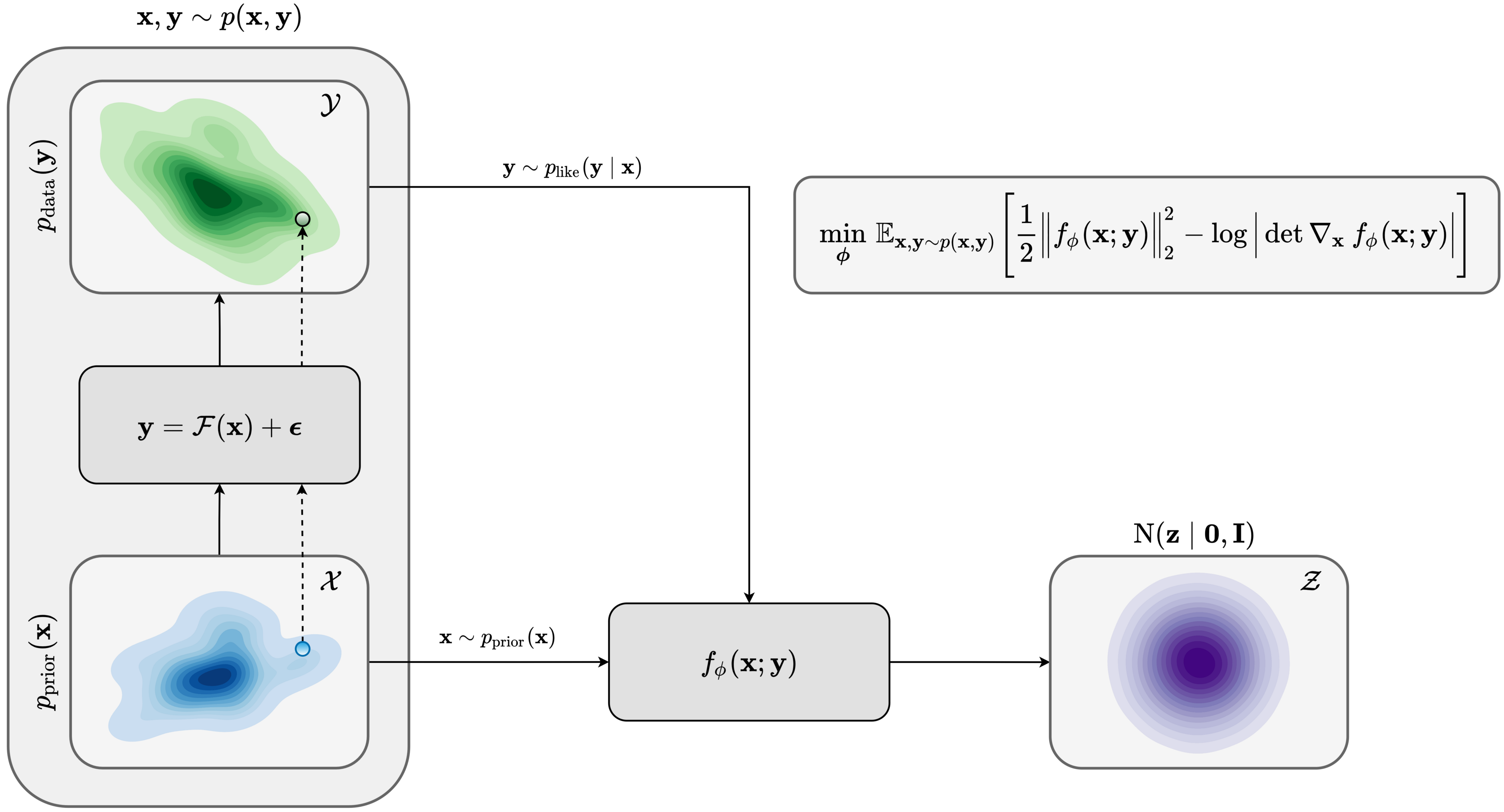
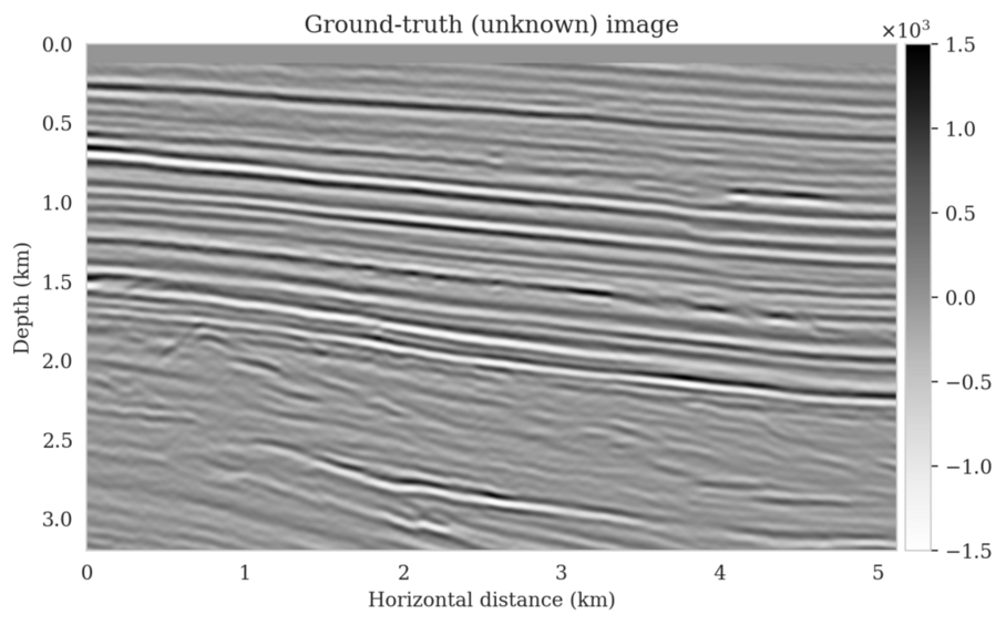
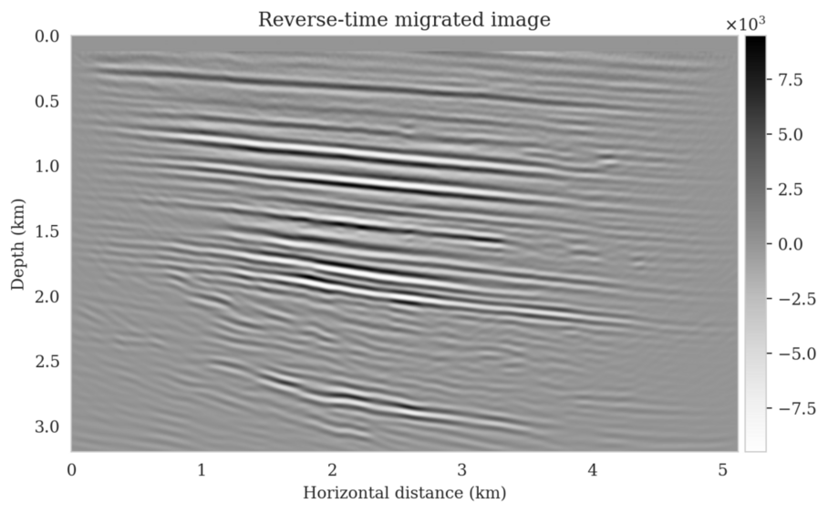
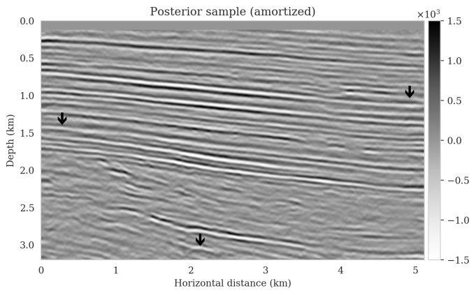
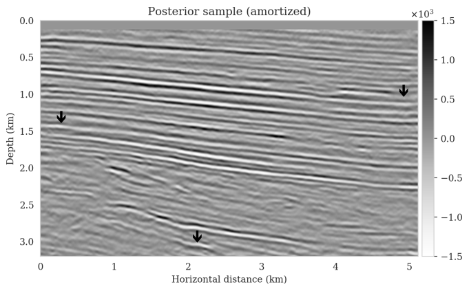
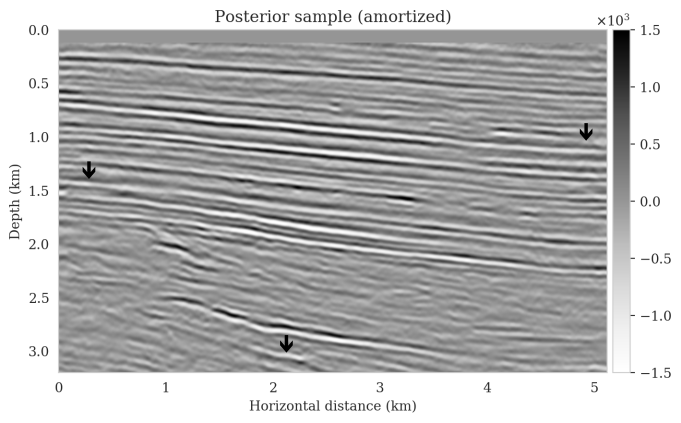
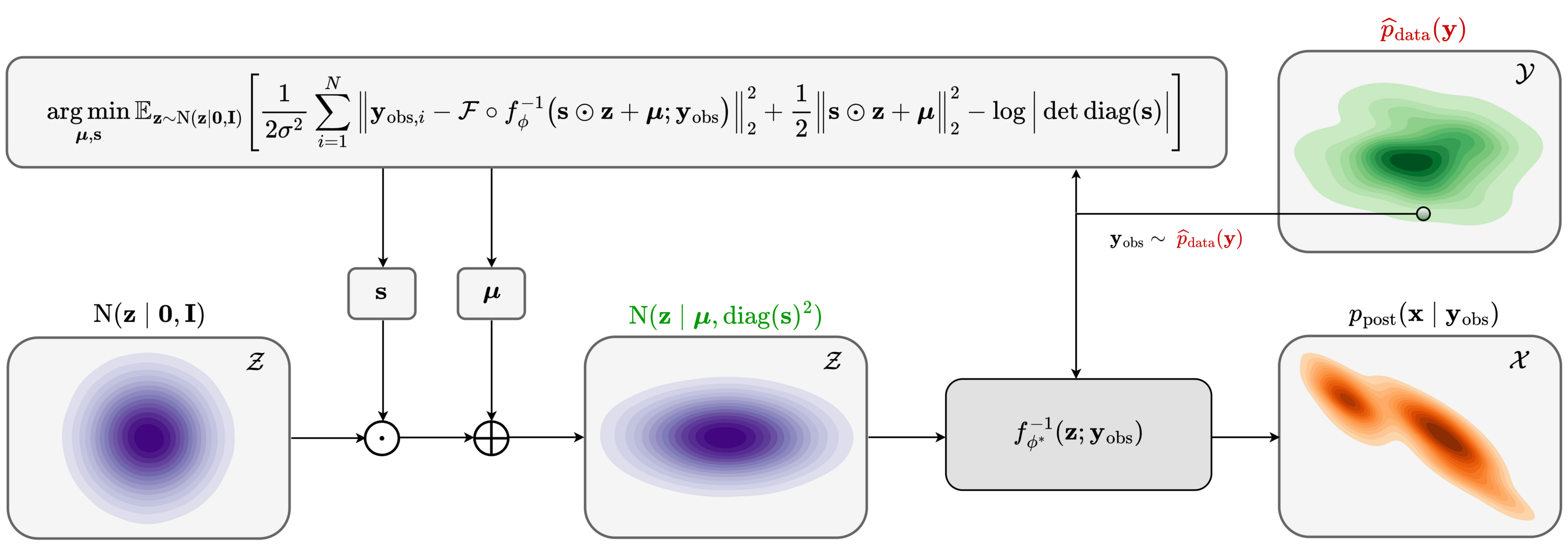
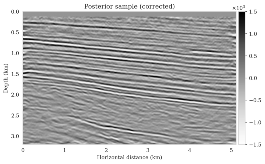
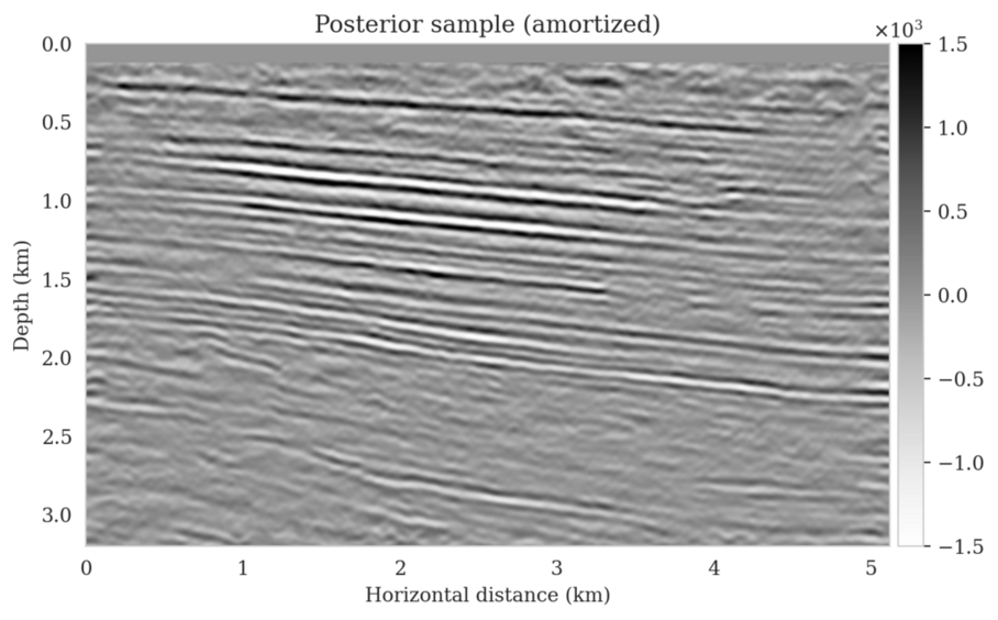
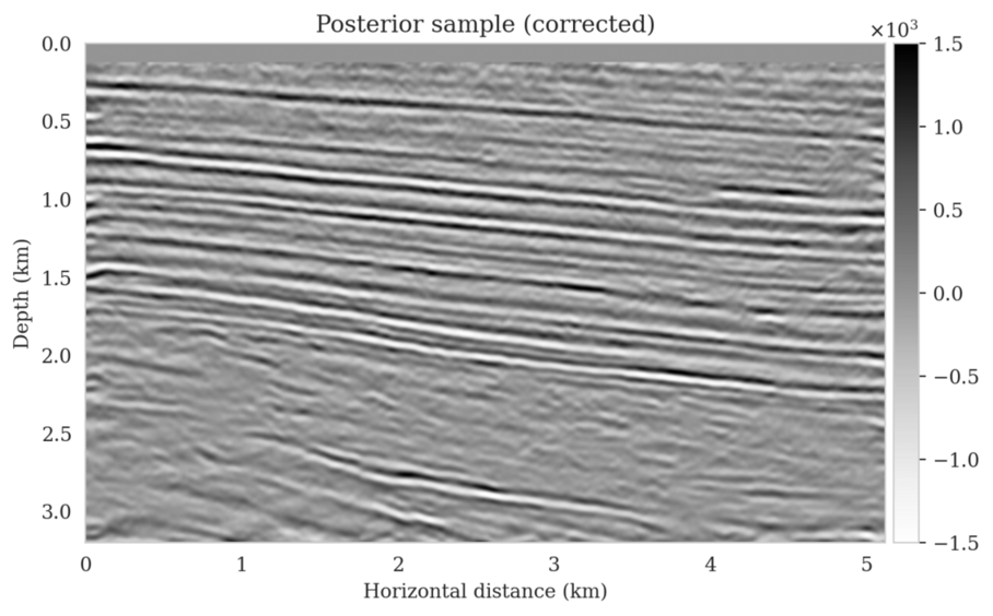
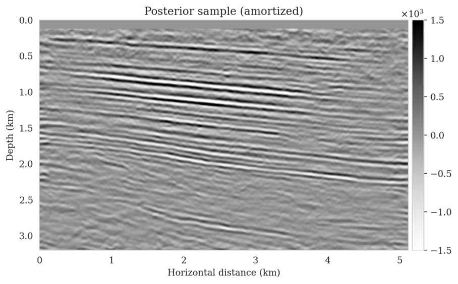
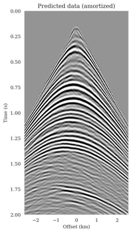
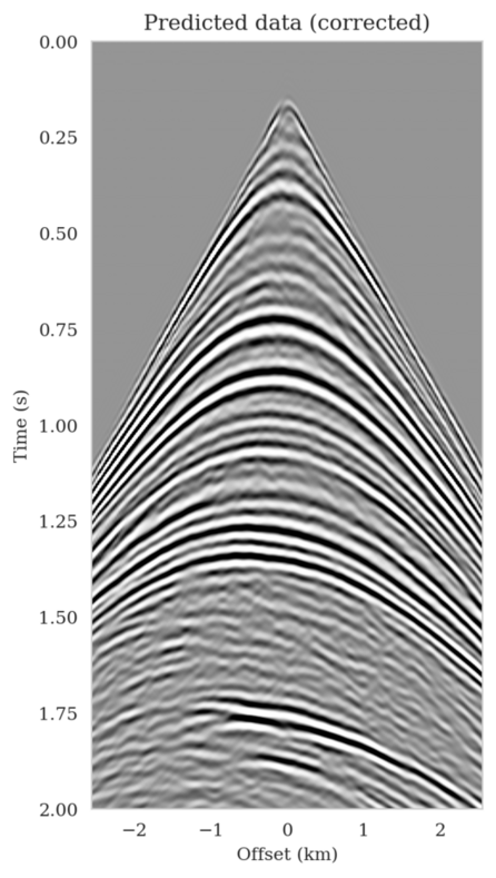
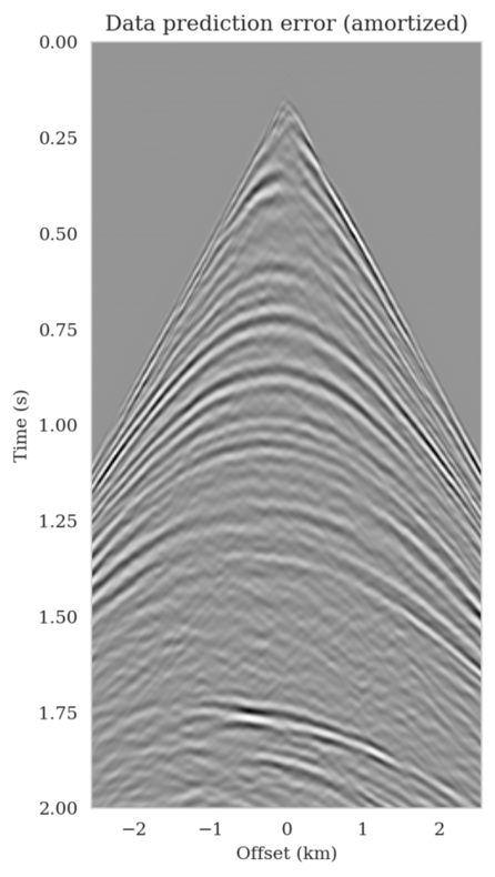
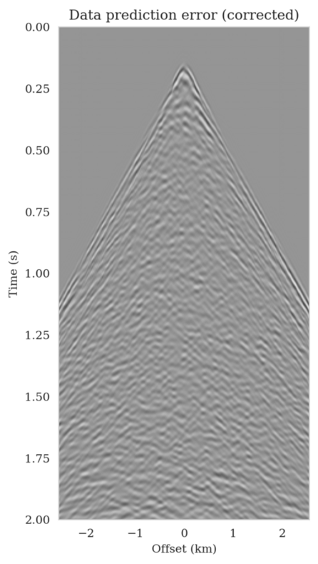
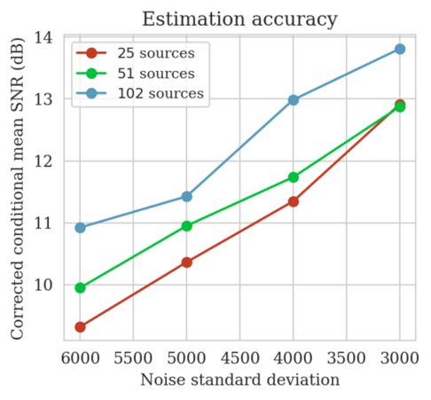
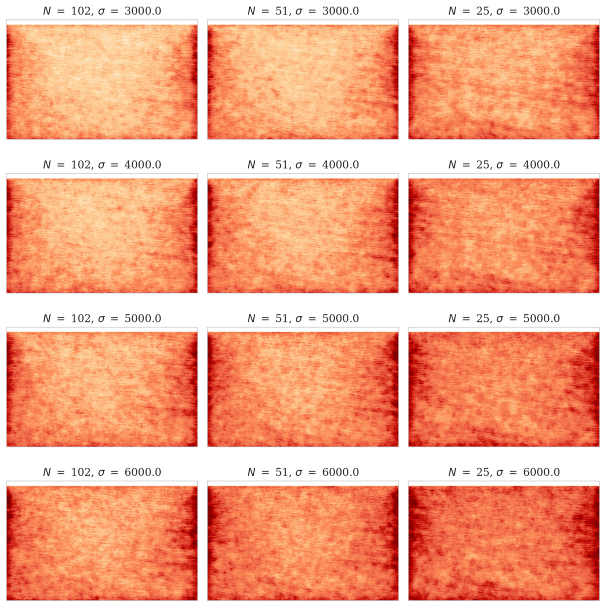
Bayesian inference for high-dimensional inverse problems is challenged by the computational costs of the forward operator and the selection of an appropriate prior distribution. Amortized variational inference addresses these challenges where a neural network is trained to approximate the posterior distribution over existing pairs of model and data. When fed previously unseen data and normally distributed latent samples as input, the pretrained deep neural network—in our case a conditional normalizing flow—provides posterior samples with virtually no cost. However, the accuracy of this approach relies on the availability of high-fidelity training data, which seldom exists in geophysical inverse problems because of the highly heterogeneous structure of the Earth. In addition, accurate amortized variational inference requires the observed data to be drawn from the training data distribution. As such, we offer a solution that increases the resilience of amortized variational inference when faced with data distribution shifts, e.g., changes in the forward model or prior distribution. Our method involves a physics-based correction to the conditional normalizing flow latent distribution to provide a more accurate approximation to the posterior distribution for the observed data at hand. To accomplish this, instead of a standard Gaussian latent distribution, we parameterize the latent distribution by a Gaussian distribution with an unknown mean and diagonal covariance. These unknown quantities are then estimated by minimizing the Kullback-Leibler divergence between the corrected and true posterior distributions. While generic and applicable to other inverse problems, by means of a seismic imaging example, we show that our correction step improves the robustness of amortized variational inference with respect to changes in number of source experiments, noise variance, and shifts in the prior distribution. This approach provides a seismic image with limited artifacts and an assessment of its uncertainty with approximately the same cost as five reverse-time migrations.

\[ \begin{equation} \begin{aligned} \Bs{\phi}^{\ast} & = \argmin_{\phi}\, \mathbb{E}_{(\B{x}, \B{y}) \sim p(\B{x}, \B{y})} \big[ -\log p_{\phi} (\B{x} \mid \B{y}) \big] \\ & = \argmin_{\phi}\, \mathbb{E}_{(\B{x}, \B{y}) \sim p(\B{x}, \B{y})} \Big[ \frac{1}{2} \left \| f_{\phi}(\B{x}; \B{y}) \right \|^2_2 - \log \Big | \det \nabla_{\B{x}} f_{\phi}(\B{x}; \B{y}) \Big | \Big]. \end{aligned} \label{vi_forward_kl_nf} \end{equation} \]

\[ \begin{equation} \begin{aligned} \Bs{\mu}^{\ast}, \B{s}^{\ast} & = \argmin_{\Bs{\mu}, \B{s}} \KL\,\big(\mathrm{N} \big(\B{z} \mid \Bs{\mu}, \operatorname{diag}(\B{s})^2\big) \mid\mid p_{\phi} (\B{z} \mid \B{y}_{\text{obs}}) \big) \\ & = \argmin_{\Bs{\mu}, \B{s}} \mathbb{E}_{\B{z} \sim \mathrm{N} (\B{z} \mid \B{0}, \B{I})} \bigg [\frac{1}{2 \sigma^2} \sum_{i=1}^{N} \big \| \B{y}_{\text{obs}, i}-\mathcal{F}_i \circ f_ {\phi} \big(\B{s} \odot\B{z} + \Bs{\mu}; \B{y}_{\text{obs}} \big) \big\|_2^2 \\ & \qquad \qquad \qquad \qquad \quad + \frac{1}{2} \big\| \B{s} \odot \B{z} + \Bs{\mu} \big\|_2^2 - \log \Big | \det \operatorname{diag}(\B{s}) \Big | \bigg ]. \end{aligned} \label{reverse_kl_covariance_diagonal} \end{equation} \]

We solve optimization problem \(\ref{reverse_kl_covariance_diagonal}\) with the Adam optimizer where we select random batches of latent variable variables \(\B{z} \sim \mathrm{N} (\B{z} \mid \B{0}, \B{I})\) and data indices. We initialize the optimization problem \(\ref{reverse_kl_covariance_diagonal}\) by \(\Bs{\mu} = \B{0}\) and \(\operatorname{diag}(\B{s})^2 = \B{I}\).

In high-dimensional inverse problems with computationally expensive forward modeling operators, Bayesian inference is challenging due to the cost of sampling the high-dimensional posterior distribution. The computational costs associated with the forward operator often limit the applicability of sampling the posterior distribution with traditional Markov chain Monte Carlo and variational inference methods. Added to the computational challenges are the difficulties associated with selecting a prior distribution that encodes our prior knowledge while not negatively biasing the outcome of Bayesian inference. Amortized variational inference addresses these challenges by incurring an offline initial training cost for a deep neural network that can approximate the posterior distribution for previously unseen observed data, distributed according to the training data distribution. When high-quality training data is readily available, and as long as there are no shifts in the data distribution, the pretrained network is capable of providing samples from the posterior distribution for previously unknown data virtually free of additional costs.

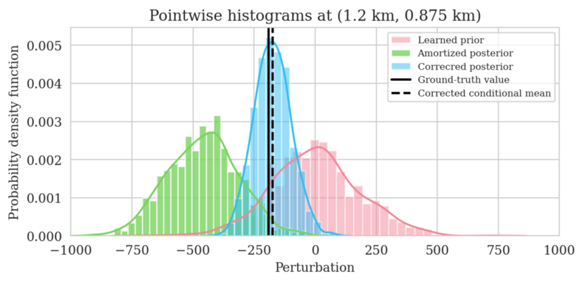
Unfortunately, in certain domains, such as geophysical inverse problems, where the structure of the Earth’s subsurface is unknown, it can be challenging to obtain a training dataset, e.g., a collection of images of the subsurface, which statistically captures the strong heterogeneity exhibited by the Earth’s subsurface. Furthermore, changes to the data generation process could negatively influence the quality of Bayesian inferences with amortized variational inferences due to generalization errors associated with neural networks. To address these challenges while exploiting the computational benefits of amortized variational inference, we proposed a data-specific, physics-based, and computationally cheap correction to the latent distribution of a conditional normalizing flow, pretrained to via an amortized variational inference objective. This correction involves solving a variational inference problem in the latent space of the pretrained conditional normalizing flow where we obtain a diagonal correction to the latent distribution such that the predicted posterior distribution more closely matches the desired posterior distribution.

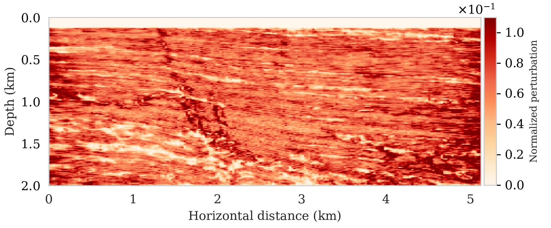
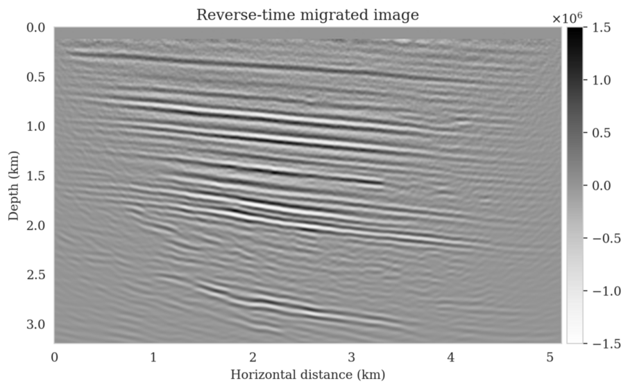
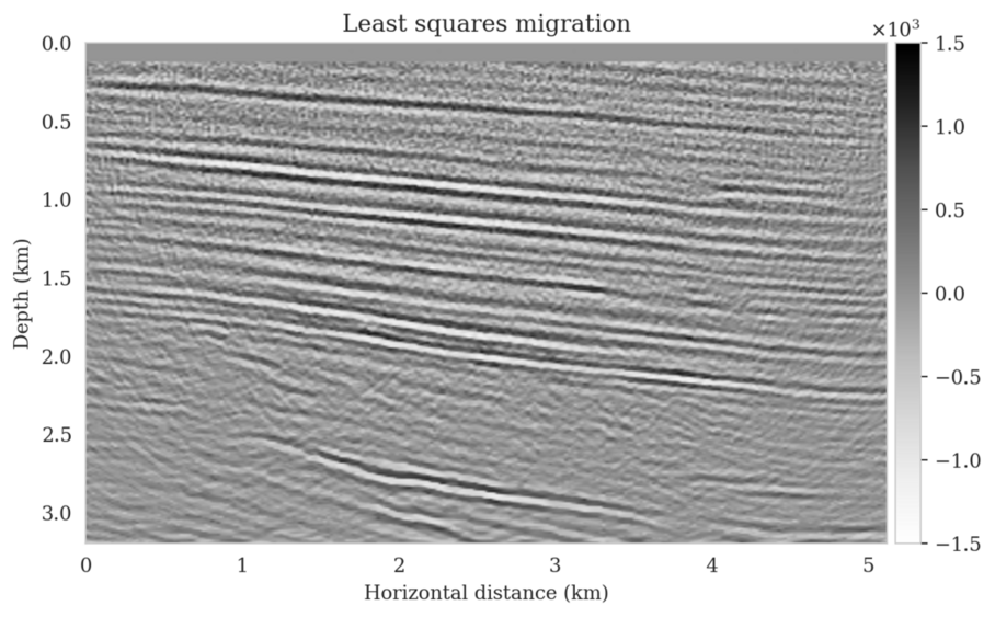
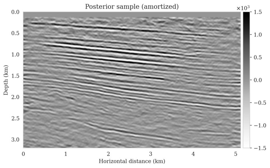
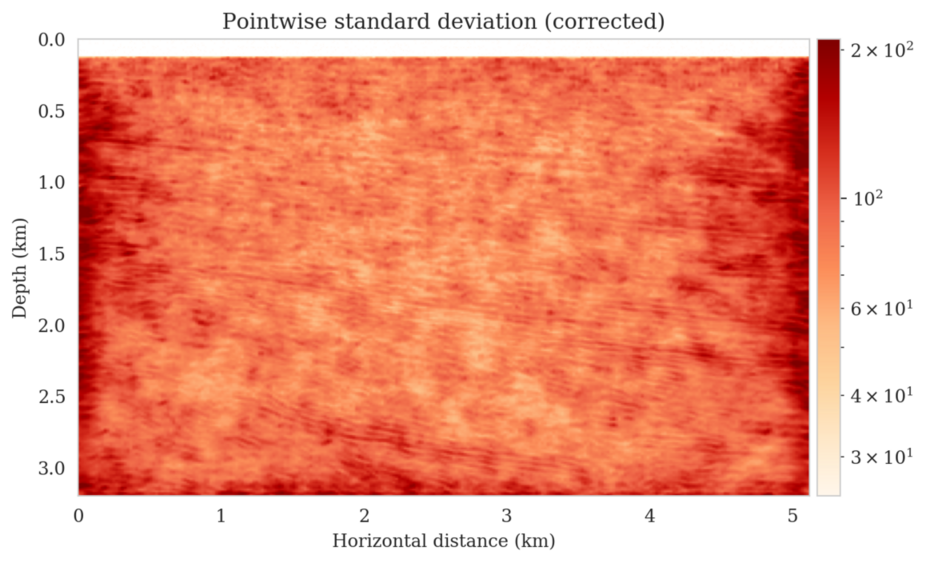
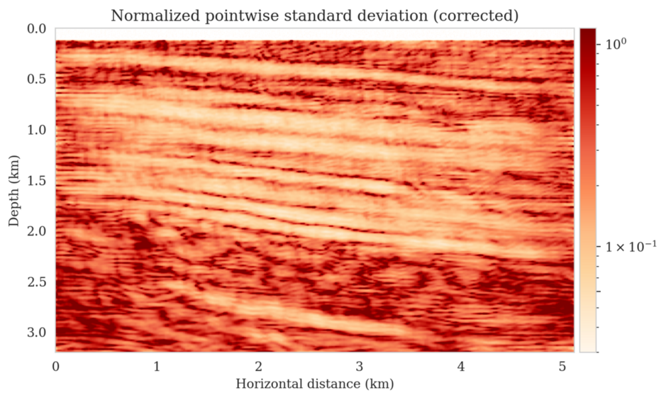
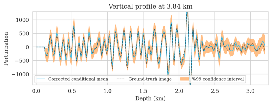
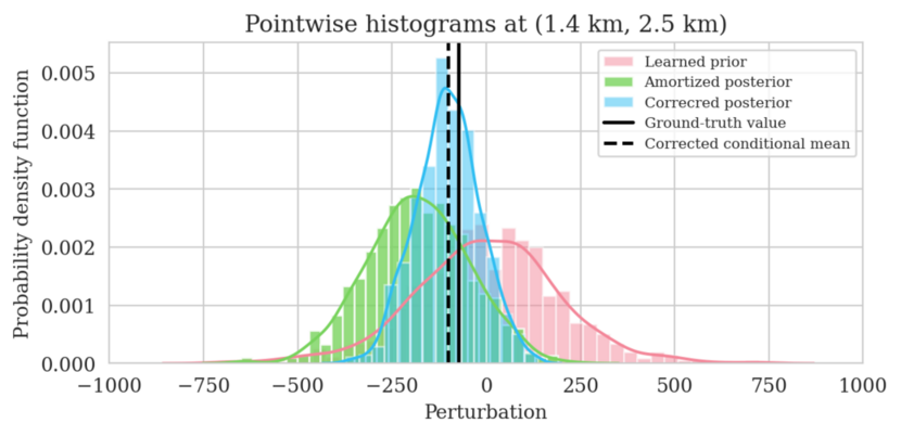
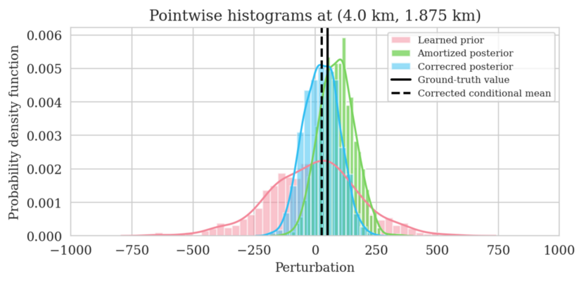
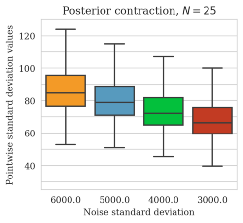
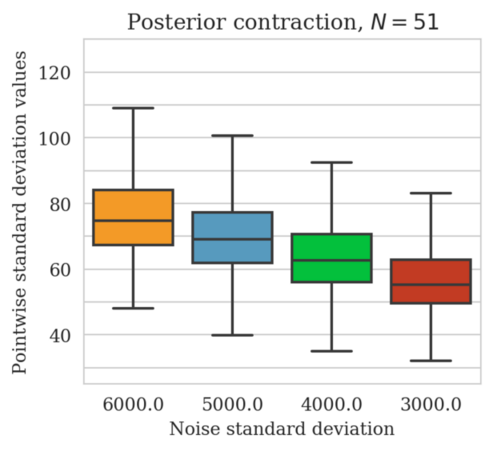
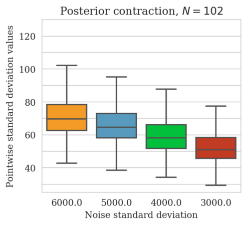
Using a seismic imaging example, we demonstrate that the proposed latent distribution correction, at a cost of five reverse-time migrations, can be used to mitigate the effects of data distribution shifts, which includes changes in the forward model as well as the prior distribution. Our evaluation indicated improvements in seismic image quality, comparable to least squares imaging, after the latent distribution correction step, as well as estimate on on the uncertainty of the image. We presented the pointwise standard deviation as a measure of uncertainty in the image, which indicated an increase in variability in complex geological areas and poorly illuminated areas. This approach will enable uncertainty quantification in large-scale inverse problems, which otherwise would be computationally expensive to achieve.

References

Siahkoohi, A., Rizzuti, G., and Herrmann, F. J., 2022, Deep bayesian inference for seismic imaging with tasks: Geophysics. Retrieved from https://slim.gatech.edu/Publications/Public/Journals/Geophysics/2022/siahkoohi2021dbif/paper.html
Siahkoohi, A., Rizzuti, G., Orozco, R., and Herrmann, F. J., 2022, Reliable amortized variational inference with physics-based latent distribution correction: Retrieved from https://arxiv.org/abs/2207.11640
Yilmaz, O., 2001, Seismic data analysis: Processing, inversion, and interpretation of seismic data: Society of Exploration Geophysicists.