
Neural networks
Introduction
As part of our multidisciplinary applied research program at SLIM and as part of ML4Seismic, we develop state-of-the-art deep-learning-based methods designed to facilitate solving a variety of scientific computing problems, ranging from geophysical inverse problems and uncertainty qualification to data and signal processing tasks commonly encountered in Imaging and Full-Waveform Inversion.
These problems are often complicated by the high dimensionality of the data and, in the case of inverse problems, by the computational complexity of the PDE-based forward modeling operators. The primary goal of our research in this area is to develop new computational methods, typically involving generative models, in order to mitigate some of these challenges. In the following section, we will briefly summarize our main contributions.
Generative Adversarial Networks1
Our main goal is to train convolutional neural networks (CNNs), \(\mathcal{G}_{\theta}: \mathcal{X} \rightarrow \mathcal{Y}\), to map unprocessed data, \(\mathcal{X}\), to processed data, \(\mathcal{Y}\). We accomplish this by estimating the networks weights, collected in the vector \(\boldsymbol{\theta}\), from training examples consisting of pairs unprocessed and processed data. Examples of processed data include wavefield reconstruction from missing traces, surface-related multiple elimination, and numerical dispersion removal.
To obtain the best performance, we use generative adversarial networks (GANs, Goodfellow et al. (2014)), which involve the training of two competing networks, namely the generator network, \(\mathcal{G}_{\theta}\), and the discriminator network, \(\mathcal{D}_{\phi}\), parameterized by the weights \(\phi\). The task of the discriminator is to discern between samples of processed data and samples from the generator obtained by mapping unprocessed data to “processed” data. The task of the generator is to fool the discriminator. As these two network perfect their game, the generator will produce samples that can not be discerned from truly processed data.
While training deep neural networks via this type of adversarial game is elegant, it can lead to instabilities during training and to disconnects between unprocessed and processed data since the discriminator is only trained to distinguish between real and fake irrespective whether the unprocessed input data and processed data are paired. To address both issues, we follow Mao et al. (2017) and Isola et al. (2017) and alternate between these two objectives: \[ \begin{equation} \begin{aligned} \min_{\boldsymbol{\theta}} &\ \mathop{\mathbb{E}}_{\mathbf{x}\sim p_X(\mathbf{x}),\, \mathbf{y}\sim p_Y(\mathbf{y})}\left [ \left (1-\mathcal{D}_{\phi} \left (\mathcal{G}_{\theta} (\mathbf{x}) \right) \right)^2 + \lambda \left \| \mathcal{G}_{\theta} (\mathbf{x})-\mathbf{y} \right \|_1 \right ] ,\\ \min_{\boldsymbol{\phi}} &\ \mathop{\mathbb{E}}_{\mathbf{x}\sim p_X(\mathbf{x}),\, \mathbf{y}\sim p_Y(\mathbf{y})} \left [ \left( \mathcal{D}_{\phi} \left (\mathcal{G}_{\theta}(\mathbf{x}) \right) \right)^2 \ + \left (1-\mathcal{D}_{\phi} \left (\mathbf{y} \right) \right)^2 \right ]. \end{aligned} \label{adversarial-training} \end{equation} \]
The expectations in the these objectives are computed with respect to existing training pairs of unprocessed and processed data, \(( \mathbf{x}_i, \mathbf{y}_i)\), drawn from the probability distributions \(p_X (\mathbf{x})\) and \(p_Y (\mathbf{y})\). To ensure that the generator maps specific paired data before and after processing, an additional \(\lambda\)-weighted \(\ell_1\)-norm penalty term is included in the objective for \(\theta\).
Examples
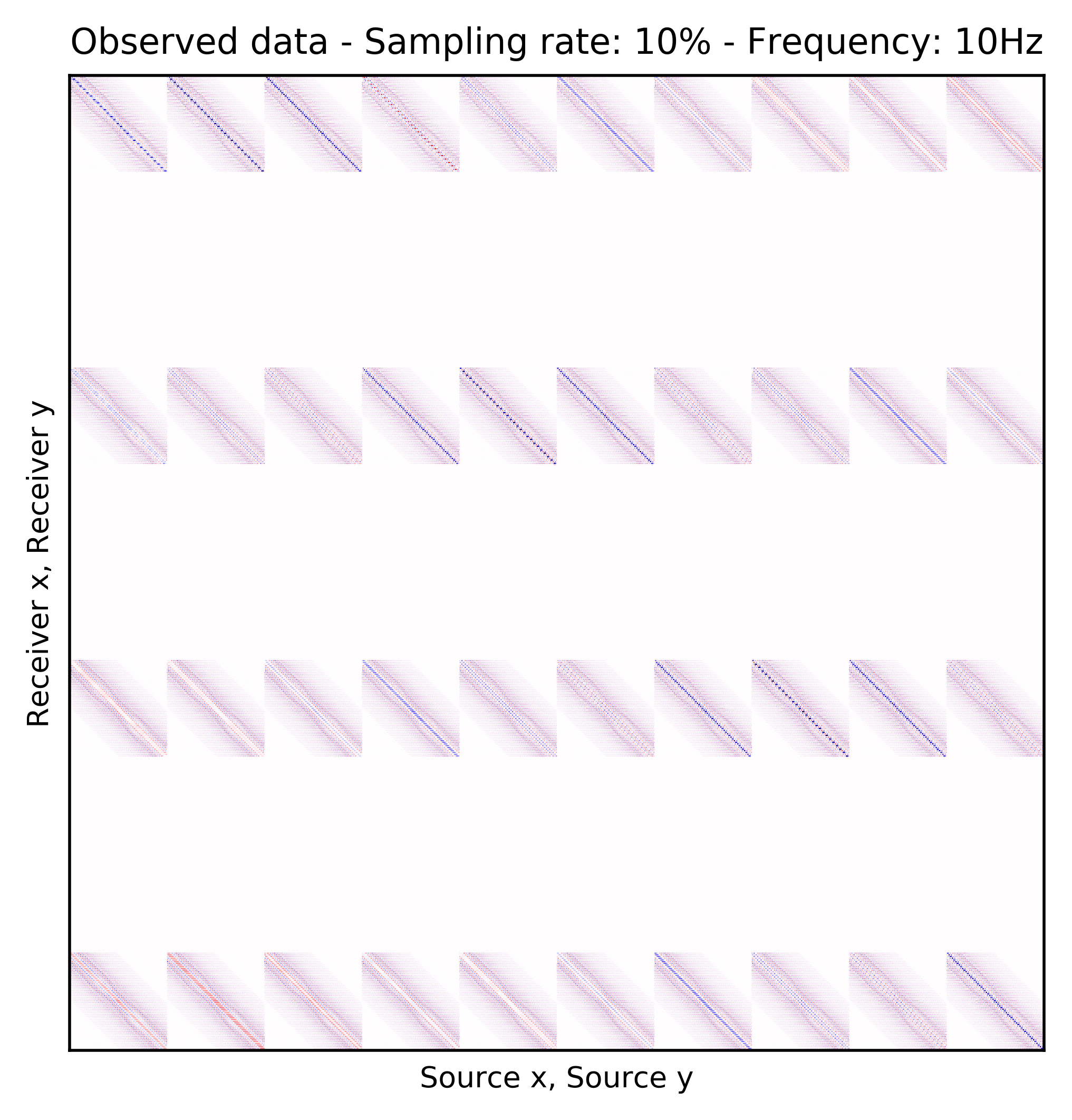
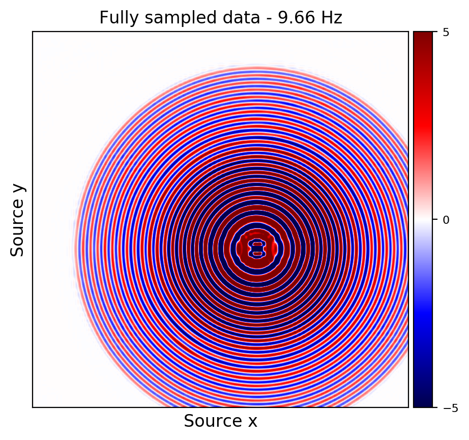
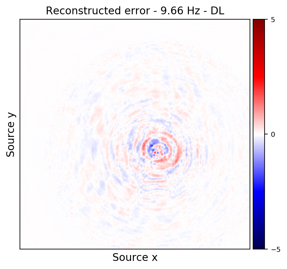
Wavefield recovery of Ocean bottom seismic data2
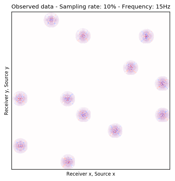
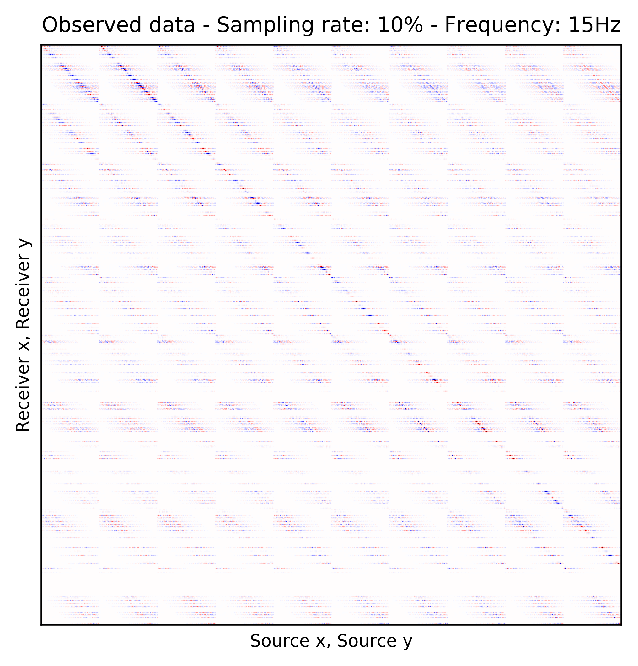
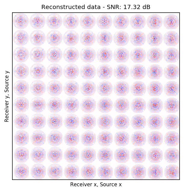
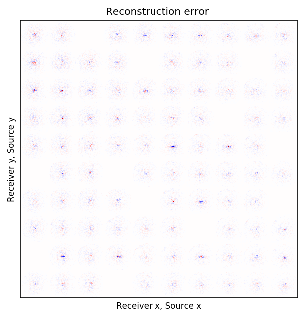
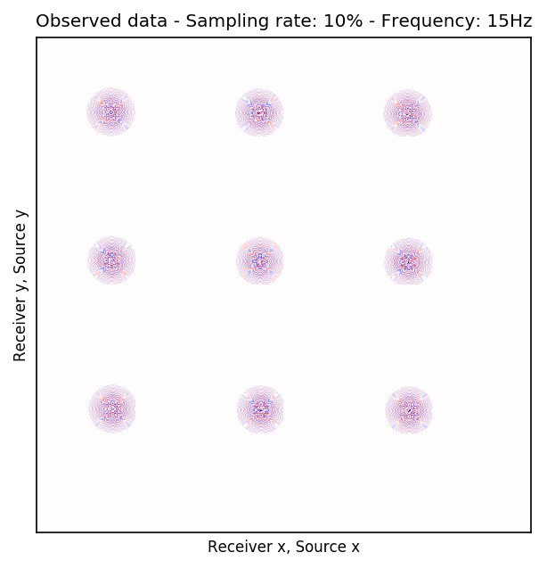
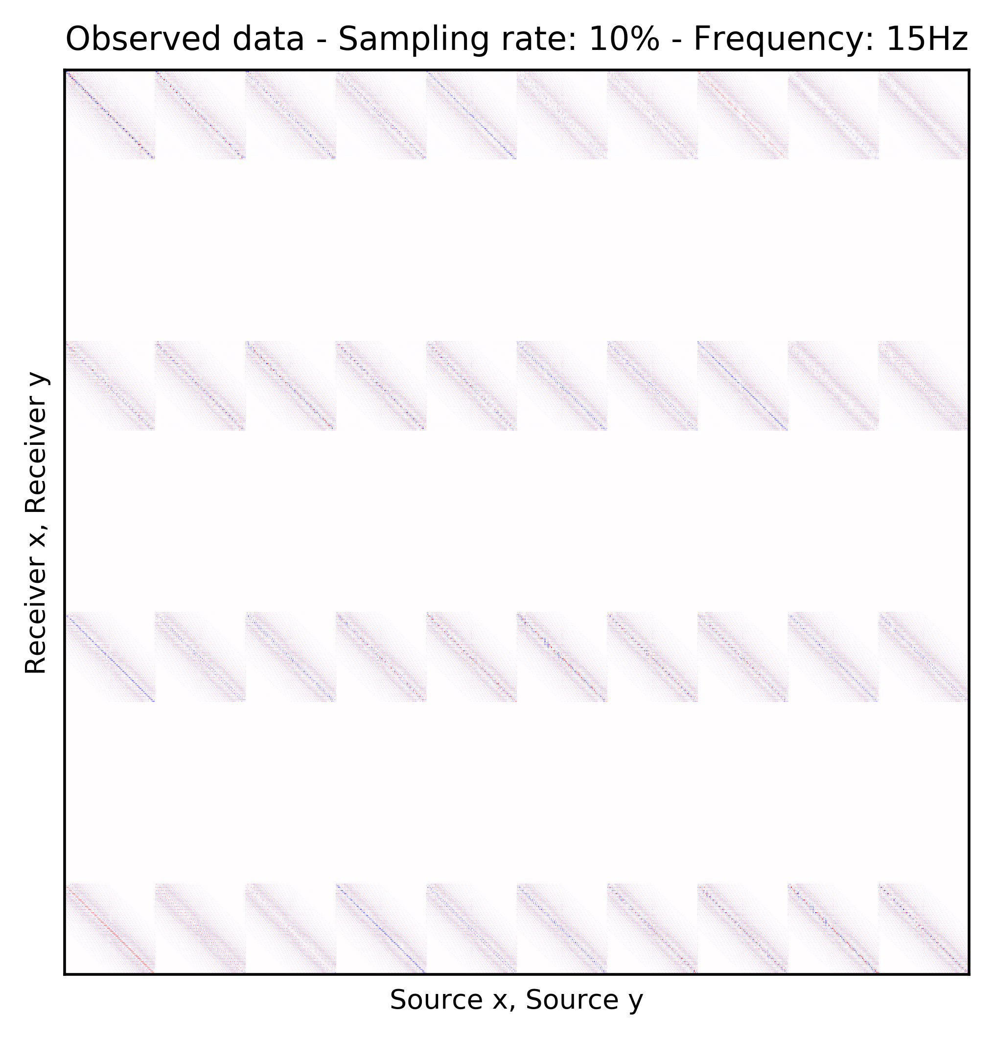
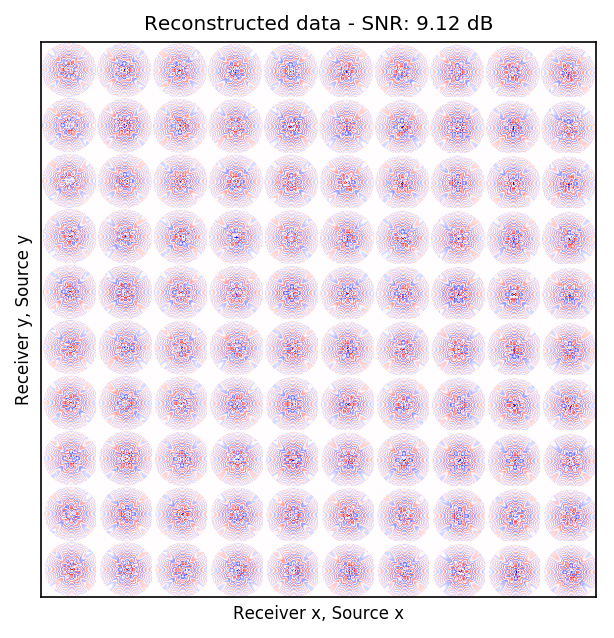
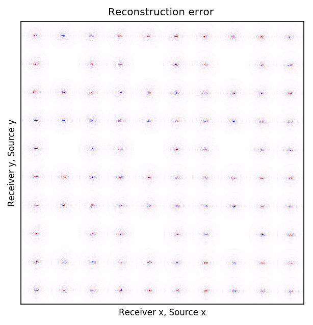
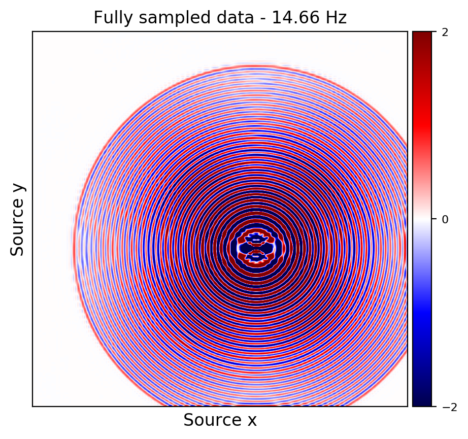
Because Ocean Bottom Nodes are expensive, node surveys typically suffer from very sparsely sampled receivers. Assuming a desirable source sampling, achievable by existing methods such as (simultaneous-source) randomized marine acquisition, we propose a deep-learning based scheme to bring the receivers to the same spatial grid as sources using a convolutional neural network. By exploiting source-receiver reciprocity, we construct training pairs by artificially subsampling the fully-sampled single-receiver frequency slices using a random training mask. After training, we deploy the neural network to fill-in the gaps in single-source frequency slices. No external training data is required and experiments on a 3D synthetic dataset demonstrate that we are able to recover receivers for up to 90% missing receivers, missing either randomly or periodically, with a better recovery for random case, at the low to midrange frequencies.
| Sampling mask | Frequency | Average recovery SNR |
|---|---|---|
| random | \(3\) Hz | \(32.66\) dB |
| random | \(5\) Hz | \(29.07\) dB |
| random | \(10\) Hz | \(23.46\) dB |
| random | \(15\) Hz | \(17.31\) dB |
| periodic | \(3\) Hz | \(32.17\) dB |
| periodic | \(5\) Hz | \(28.32\) dB |
| periodic | \(10\) Hz | \(20.82\) dB |
| periodic | \(15\) Hz | \(9.12\) dB |
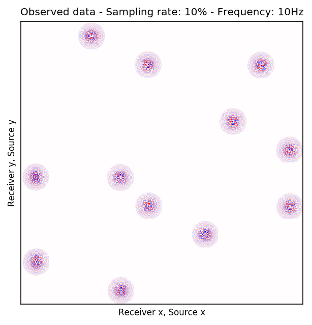
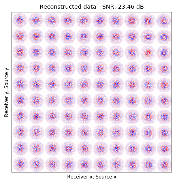
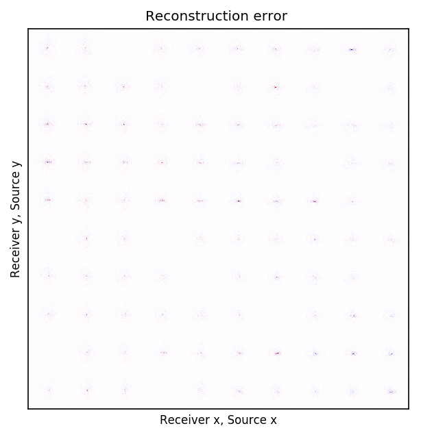
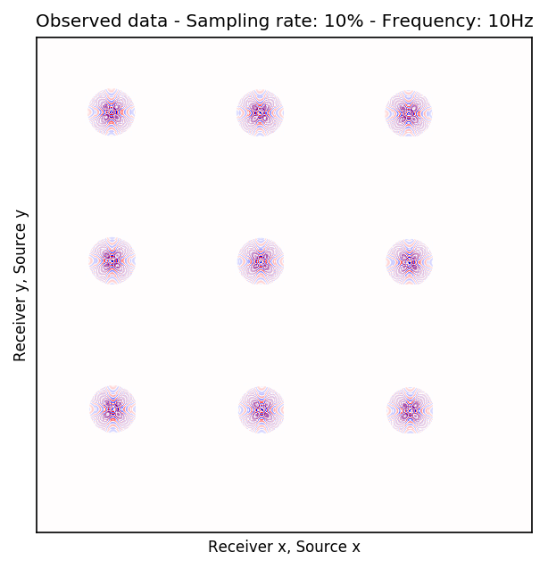
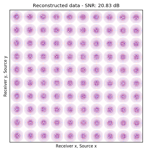
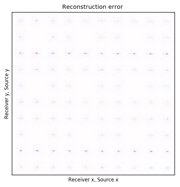
An important distinction of this contribution compared to similar works is that it does not need any external training data. This is accomplished by assuming that source-receiver reciprocity holds and that the sources are densely sampled. These assumptions are reasonable when relying on existing survey techniques such as (simultaneous-source) randomized marine acquisition. While this approach has been used successfully for the recovery monochromatic frequency slices, its application in practice calls for wavefield reconstruction of time-domain data. Despite having the option to parallelize, the overall costs of this approach can become prohibitive if we decide to carry out the training and recovery independently for each frequency slice. Because different frequency slices share information, we propose the use the method of transfer training to make our approach computationally more efficient by warm starting the training with CNN weights obtained from a neighboring frequency slices. We show this principle by carrying a series of carefully selected experiments on a relatively large-scale five-dimensional data synthetic data volume associated with wide-azimuth 3D ocean bottom node acquisition.
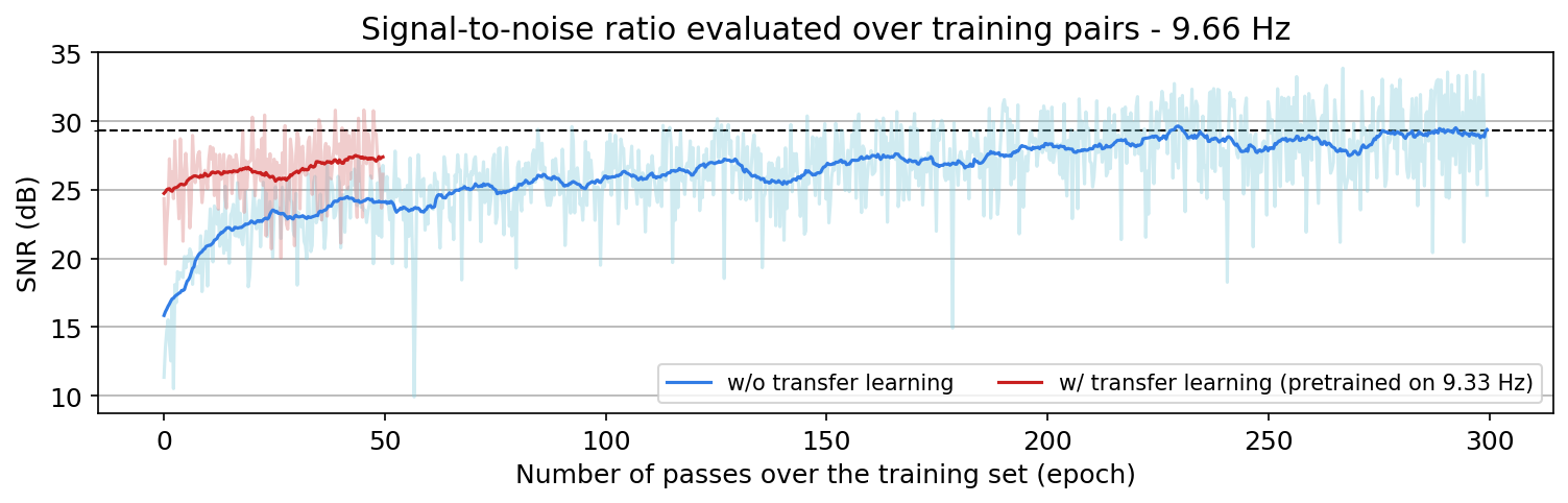
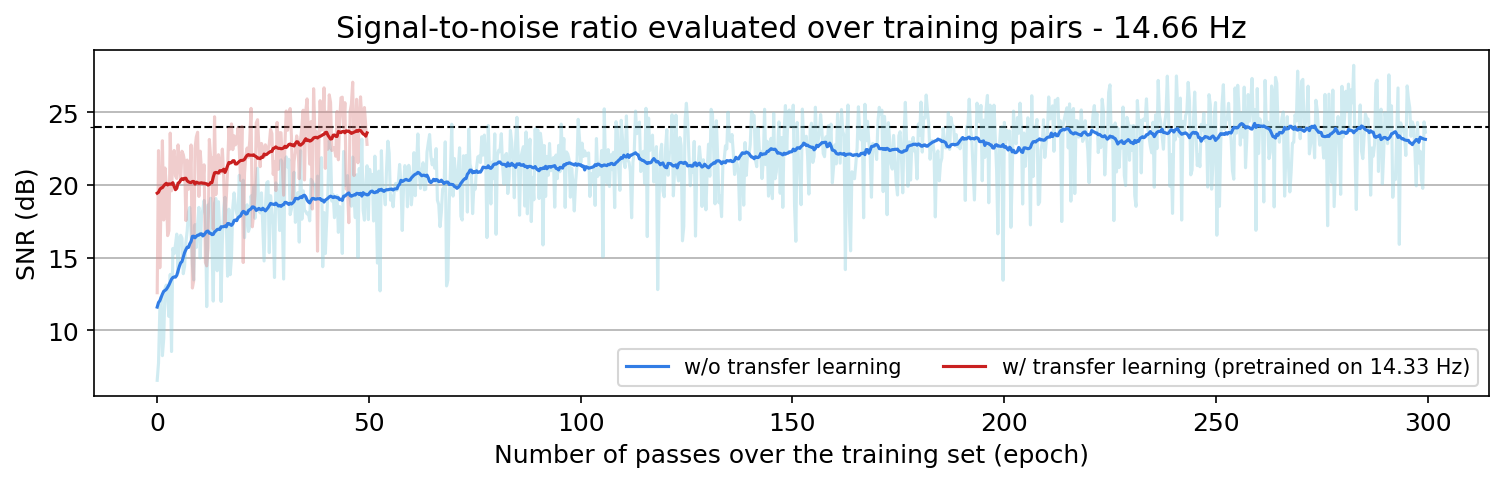
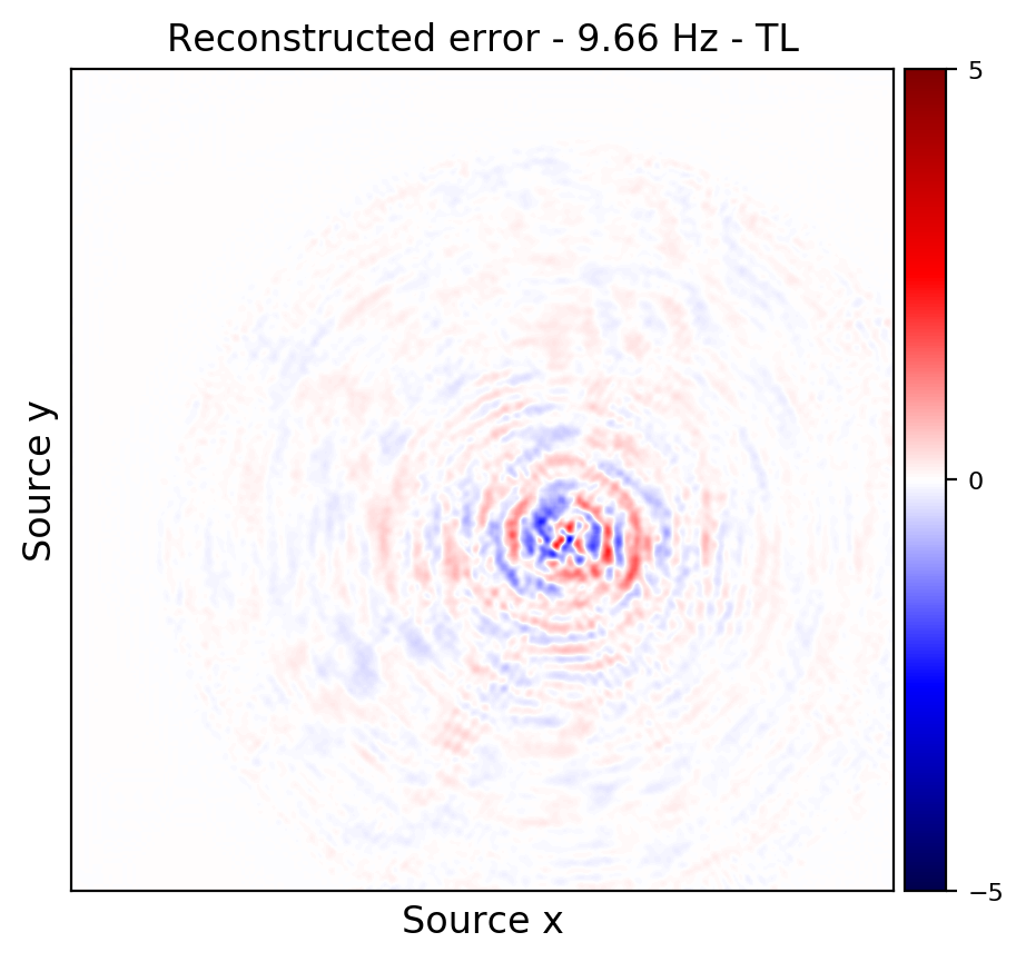
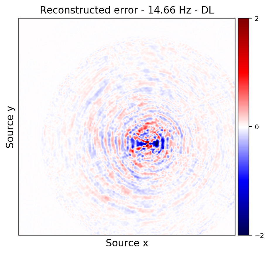
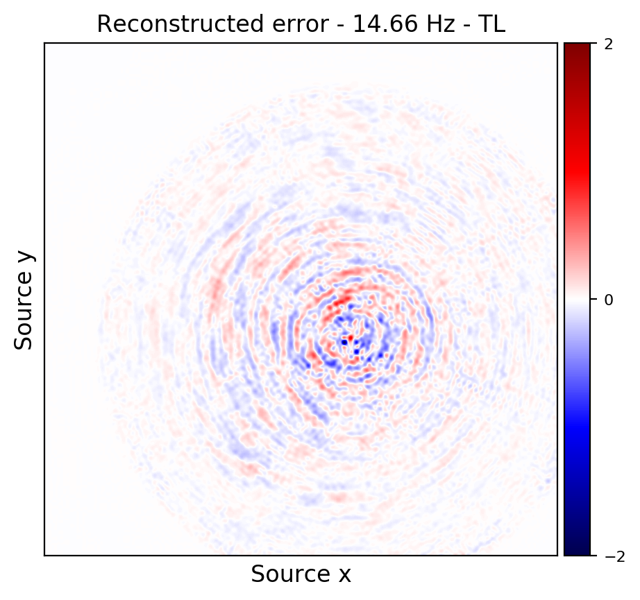
From these experiments, we observe that by transfer training we are able t significantly speedup in the training, specially at relatively higher frequencies where consecutive frequency slices are more correlated.
Invertible Networks
An important consideration when training neural networks on large dimensional data is the memory footprint that they incur during training. Backpropagation on neural networks will require to save in memory the intermediate activation of the data at each intermediate layer. Deep learning has shown that we can expect higher quality results as the depth of a network is increased, but increasing the number of layers in the network reach a limit where the network can no longer be trained on the GPU resources available. This problem is highlighted when performing machine learning on 3D volumes. To remedy this problem, we propose the use of invertible networks. This subset of neural networks are designed such that the intermediate states can be computed from the output of the network. Thus intermediate states are not saved and large memory gains are achieved.
This principle of invertibility is important for memory concerns but they also allow for distribution learning with change of variable based training paradigms. These methods have gained recent popularity with their implementations as Normalizing Flows. We implement invertible networks for memory efficient supervised learning and also normalizing flows in our package InvertibleNetworks.jl.
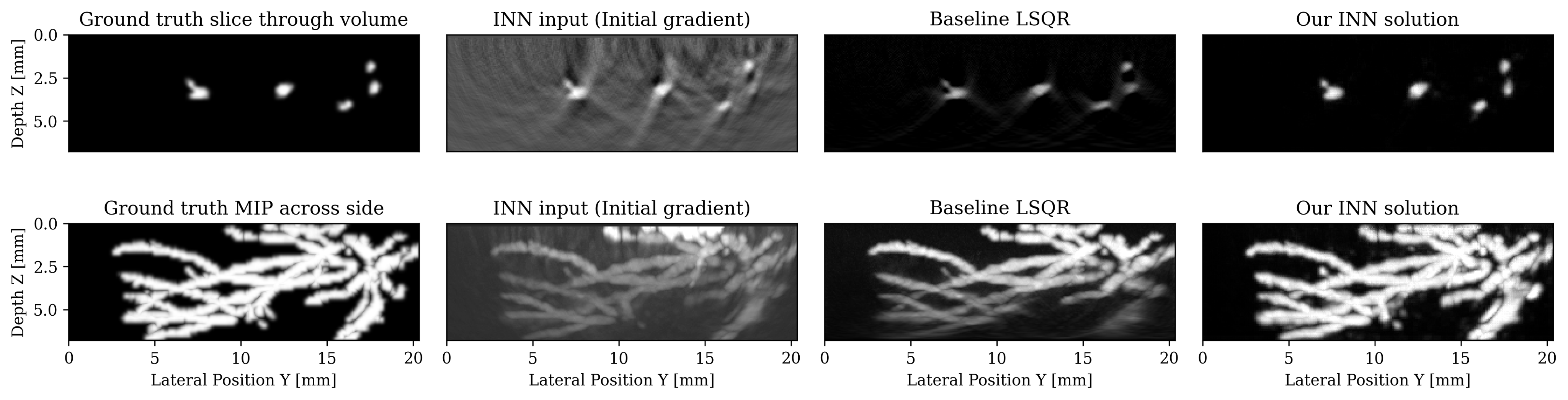
Memory efficient data-driven 3D Photoacoustic imaging
As an application, we tackle 3D photoacoustic imaging in the case of limited-view, noisy and subsampled data, that makes the inverse problem ill-posed. Multiple solutions \(x\) can explain the data \(y\), therefore, this problem is typically solved in a variational framework where prior knowledge of the solution is incorporated by solving the minimization of the combination of an \(\ell_2\) data misfit \(L\) and a regularization term \(p_{\mathrm{prior}}(x)\). The success of this formulation hinges on users carefully selecting hyperparameters by hand such as the optimization step length and the prior itself, typically a multipurpose generic prior such as TV norm. On the other hand, recent machine learning work argues that we can learn the optimal step length and even a prior. We pursue this avenue and select loop-unrolled networks since this learned method also leverages the known physics of the problem encoded in the model \(A\).
Loop unrolled networks emulate gradient descent where the \(i^{\text{th}}\) update is reformulated as the output of a learned network \(\Lambda_{\theta_{i}}\): \[ \begin{equation} x_{i+1}, s_{i+1} = \Lambda_{\theta_{i}}(x_{i},s_{i}, \nabla_{x}L(A,x_{i},y)) \label{eq:loopunrolled} \end{equation} \] where \(s\) is a memory variable and \(\nabla_{x}L\) is the gradient w.r.t the data misfit on observed data \(y\). In our photoacoustic case, \(A\) is a linear operator (discrete wave equation) and \(L\) is \(\ell_2\) norm data misfit so the desired gradient is \(\nabla_{x}L(A,x_{i},y) = A^{\top}(Ax_{i}-y)\). Thus, each gradient will require two PDE solves: one forward and one adjoint. These wave propagations embed the known physical model into the learned approach. show that this method gives promising results on 3D photoacoustic but note that they are limited to training shallow networks due to memory constraints. To improve on this method, we propose using an INN that is an invertible version of loop-unrolled networks.
Our invertible neural network (INN) is based on the work of Putzky et al. (2019), where they propose an invertible loop-unrolled method called invertible Recurrent Inference Machine (i-RIM). While typical loop-unrolled approaches have linear memory growth in depth Hauptmann et al. (2018), i-RIM has constant memory usage due to its invertible layers. A network constructed with invertible layers does not need to save intermediate activations thus trading computation cost required to recompute activations for extremely frugal memory usage. We adapt i-RIM to Julia and make our code available alongside other invertible neural networks at InvertibleNetworks.jl Witte et al. (2020).
Normalizing Flows
In a landscape that is dominated by GANs, Normalizing Flows offer a noteworthy alternative for generative models. As generative models, Normalizing Flows offer straight forward training thanks to their exact likelihood evaluation capabilities, and also have fast sampling at test time. The intrinsic invertibility of these models allows for memory efficient training which was their initial motivation of their implementation in InvertibleNetworks.jl.
The formula central to Normalizing Flows and other flow models is the change of variables formula: \[ \begin{equation} p_x(x) = p_z(f_\theta(x)) \, \left| \, \det \frac{\partial f_\theta}{\partial x}\right|. \label{eq:changevariables} \end{equation} \] Where \(p_x\) is called the target distribution (typically a complex/multimodal distribution), \(p_z\) is called the base distribution and is a simple distribution, and \(f_\theta\) is a function that is capable of transforming samples from the \(\mathbf{X}\) space to \(\mathbf{Z}\) space.
The derivation of this formula can be found in many places as this is a well known relation that comes from the fact that the density of a sample in the \(\mathbf{X}\) space must be equal to the density of that sample transformed into the \(\mathbf{Z}\) space even if the volume of the sample changes. The Jacobian term is what controls for this change in volume.
Practically, this formula allows us to evaluate the likelihood of a sample \(x\) after transforming through a function \(f_{\theta} : \mathbf{X} \rightarrow \mathbf{Z}\).
To see why we would want to do this, imagine that \(p_x(x)\) represents the distribution of human faces. Then it is clear that we can’t evaluate \(p_x(x)\) for a given face \(x\) but what if we were given a magical \(f_{\theta}\) that transforms the face \(x\) into Normally distributed white noise \(z\). Then the change of variable formula allows us to evaluate the likelihood in this simple distribution (log-likelihood is just the \(\ell_2\) norm) as long as we control for the change of volume caused by the function \(f_{\theta}\) in other words the determinant of the Jacobian term \(\left| \det \frac{\partial f_\theta}{\partial x} \right|\).
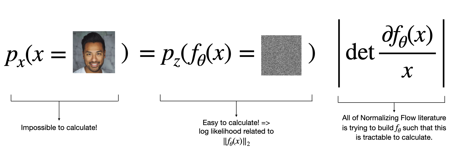
This likelihood evaluation of a complex distribution in a simple/known distribution is what gives us a maximum likelihood framework for training our parameterized functions \(f_{\theta}\) which we will parameterize as a Normalizing Flow.
Training a Normalizing Flow
Normalizing Flow training is based on likelihood maximization of the parameterized model \(f_{\theta}\) under the log-likelihood of samples from a data distribution \({x} \sim p_{x}(x)\): \[ \begin{equation} \underset{\mathbf{\theta}}{\operatorname{argmax}} \mathbb E_{{x} \sim p_{x}(x)} [\log p_{x}(x)]. \label{eq:NFderiv1} \end{equation} \] We make this a minimization problem by looking at the negative log-likelihood and then use the change of variables formula to express the likelihood on a transformed sample \(f_\theta({x})\) in the latent space \(Z\) which we will take to be the standard Normal distribution \(z \sim \mathcal{N}(0,I)\): \[ \begin{equation} \underset{\mathbf{\theta}}{\operatorname{argmin}} E_{{x} \sim p_{x}(x)} -\log p_{x}(x) = \underset{\mathbf{\theta}}{\operatorname{argmin}} E_{{x} \sim p_{x}(x)} -\log \left[ p_{z}(f_\theta(x)) \, \left|\det \frac{\partial f_\theta}{\partial x}\right| \right] \label{eq:NFderiv2} \end{equation} \] \[ \begin{equation} = \underset{\mathbf{\theta}}{\operatorname{argmin}} E_{{x} \sim p_{x}(x)} -\log p_{z}(f_\theta(x)) \, -\log \, \left|\det \frac{\partial f_\theta}{\partial x}\right|. \label{eq:NFderiv3} \end{equation} \] Note that since we are evaluating the negative log-likelihood of a sample which is Normally distributed \(-\log p_{z}(f_\theta(x))\) we simply evaluate its \(\ell_2\) norm \[ \begin{equation} = \underset{\mathbf{\theta}}{\operatorname{argmin}} E_{{x} \sim p_{x}(x)} \left[\frac{1}{2}\|f_\theta({x})\|_2^2 - \log \, \left| \, \det \frac{\partial f_\theta}{\partial x} \, \right| \, \right]. \label{eq:NFderiv4} \end{equation} \] We evaluate the expectation \(E_{{x} \sim p(x)}\) with the Monte Carlo approximation using samples from a training dataset \(X_{train}\) that has been sampled from the true distribution: \[ \begin{equation} \underset{\mathbf{\theta}}{\operatorname{argmin}} \frac{1}{N} \sum_{x \in X_{train}} \left[\frac{1}{2}\|f_\theta({x})\|_2^2 - \log \, \left| \, \det \frac{\partial f_\theta}{\partial x} \, \right| \, \right]. \label{eq:NFderiv5} \end{equation} \] This is our final training objective and it tells an extremely intuitive story: apply your network to your data \(\hat z = f_\theta(x)\) and minimize its \(\ell_2\) norm while also maximizing the term involving the determinant of the Jacobian. If we interpret this Jacobian term as measuring the “expansion” of density space caused by the network then we are making sure that the learned probability does not collapse on single modes giving a peaky distribution.
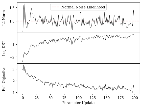
The above figure shows a typical scenario in Normalizing Flow training where we are tracking the values of the two terms that make up the full objective. In the first row, we show the \(\ell_2\) norm of samples, and in the second row we show the value of the Jacobian term. At first glance we would think that minimizing the \(\ell_2\) norm of samples would simply train the network to map samples to zero. But from studying a training log of these terms we can see that the \(\ell_2\) norm of samples instead starts to converge to the value of the expected norm of samples that come from a Normal distribution namely \(1\). This is thanks to the Jacobian term which is continually battling to “expand” the output distribution.
Fourier Neural Operators
Our contribution to this research area revolves mainly around risk mitigation of Geological Carbon Storage through the use of numerical surrogate models to solve uncertainty quantification and inverse problems relating to the long-term behavior of injected CO\(^2\) in the Earth’s subsurface.
Domain-decomposed Fourier Neural Operators as Large-scale Numerical Surrogates
(In Prepublication here, Software available here)
Fourier Neural Operators (FNOs) are a graph neural network architecture first (proposed; Z. Li et al., 2020) by Li et al. which have been shown to be effective numerical surrogates for the solution operator to elliptic or systems of elliptic PDEs. In this context, FNOs attempt to learn the mapping \[ \begin{equation} \mathcal{G}: \mathcal{A} \times \Theta \rightarrow \mathcal{U} \label{fno_mapping} \end{equation} \] where \(\mathcal{A}, \Theta,\) and \(\mathcal{U}\) are function spaces containing the input, parameters, and output of the solution to the PDE in question.
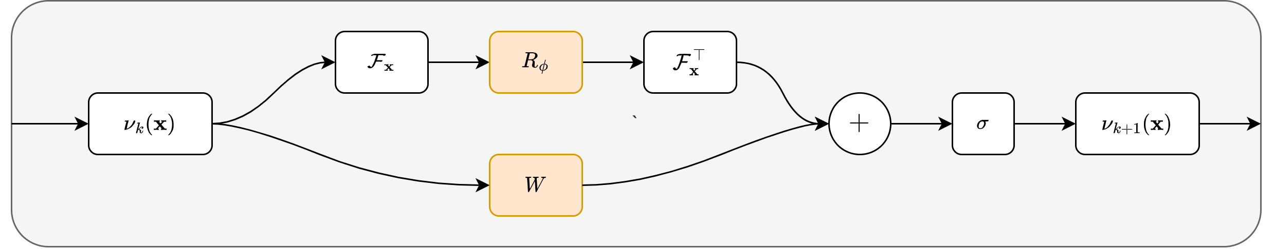
FNOs construct a sequence of functions \(\nu_1(\mathbf{x}), \dots, \nu_K(\mathbf{x})\) using \(K\) blocks, each of which act on vectors \(\mathbf{x} \in \R^d\), a lifted space larger than the size of the input space. These blocks consist of two component pieces: the spectral convolution, which uses a low-pass filter and learned elementwise transformation in Fourier space, and a pointwise linear transformation along the lifted dimension \(d\). The outputs of these components are then added together and passed through a nonlinearity. A diagram of this is illustrated below.
One key issue with using FNOs for problems of a realistic size (e.g. approximating solutions to the 3D time-varying two-phase flow equations as part of a larger CCS workflow) is that they require both the data and model weights to scale to sizes too large to fit inside of the memory of a single GPU during both training and inference. This is in contrast to other machine learning models such as transformers, wherein the model grows in size while the size of each data point remains relatively constant. Additionally, FNOs act on volumetric, high-dimensional data (6D batch \(\times\) channels \(\times x \times y \times z \times t\) for 3D time-varying outputs), and thusly require a different parallelism strategy than the traditional data and pipeline parallelism used in more standard machine learning applications.
To remedy this problem, we propose to use domain-decomposition techniques more akin to those found in classical HPC applications (e.g. adaptive mesh PDE solvers) to introduce model parallelism via splitting of the input data and network weights along their respective spacetime dimensions onto many computational workers. This allows memory usage on each worker to remain effectively constant and the network to therefore scale to problems of arbitrary size. To deal with the complexities of domain-decomposition based parallelism in neural networks, we adopt the linear algebraic abstractions (described; Russell J Hewett et al., 2021) by Hewett et al. and implemented using (DistDL; Russell J. Hewett et al., 2021). Here, computational and parallel primitives are described as linear operators acting on a vectorization of a supercomputer’s memory, and can then be cleanly used to describe complex parallel algorithms and their adjoints used in distributed machine learning applications.
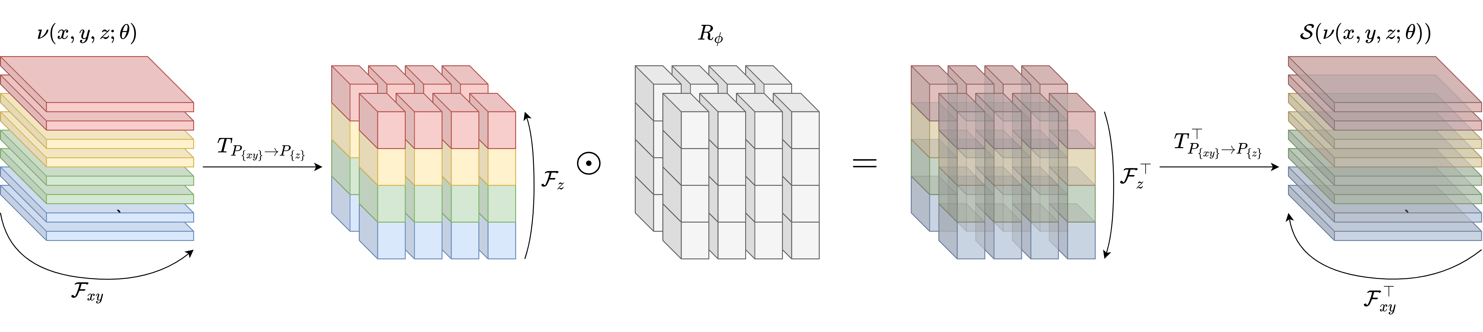
In the context of FNOs, this parallelism is most present in the spectral convolution \(\mathcal{S}\nu = \mathcal{F}^\top R_\phi \mathcal{F} \nu\). Specifically, because \(R_\phi\) is applied elementwise, the largest amount of parallel communication is present in the Fourier and adjoint Fourier transforms. Distributed Fourier transforms are a well-studied problem, with modern (approaches; Dalcin et al., 2018) exploiting the separability of the Fourier transform to compute sequential fast Fourier transforms (FFTs) along particular dimensions or sets of dimensions with all-to-all (what we refer to as repartition) operations in between each transformation. An illustration of this on 3D data \((x,y,z)\) is shown below in Figure 8.
Because this distributed FFT has been implemented using DistDL inside of PyTorch, everything is fully differentiable and allows for sensitivitites to be computed w.r.t parameters, even in a multi-node distribution setting. This ultimately allows for integration into a larger gradient-based optimization or inversion framework, opening the possibility for previously intractible large-scale uncertainty quantification and inversion problems to be solved.
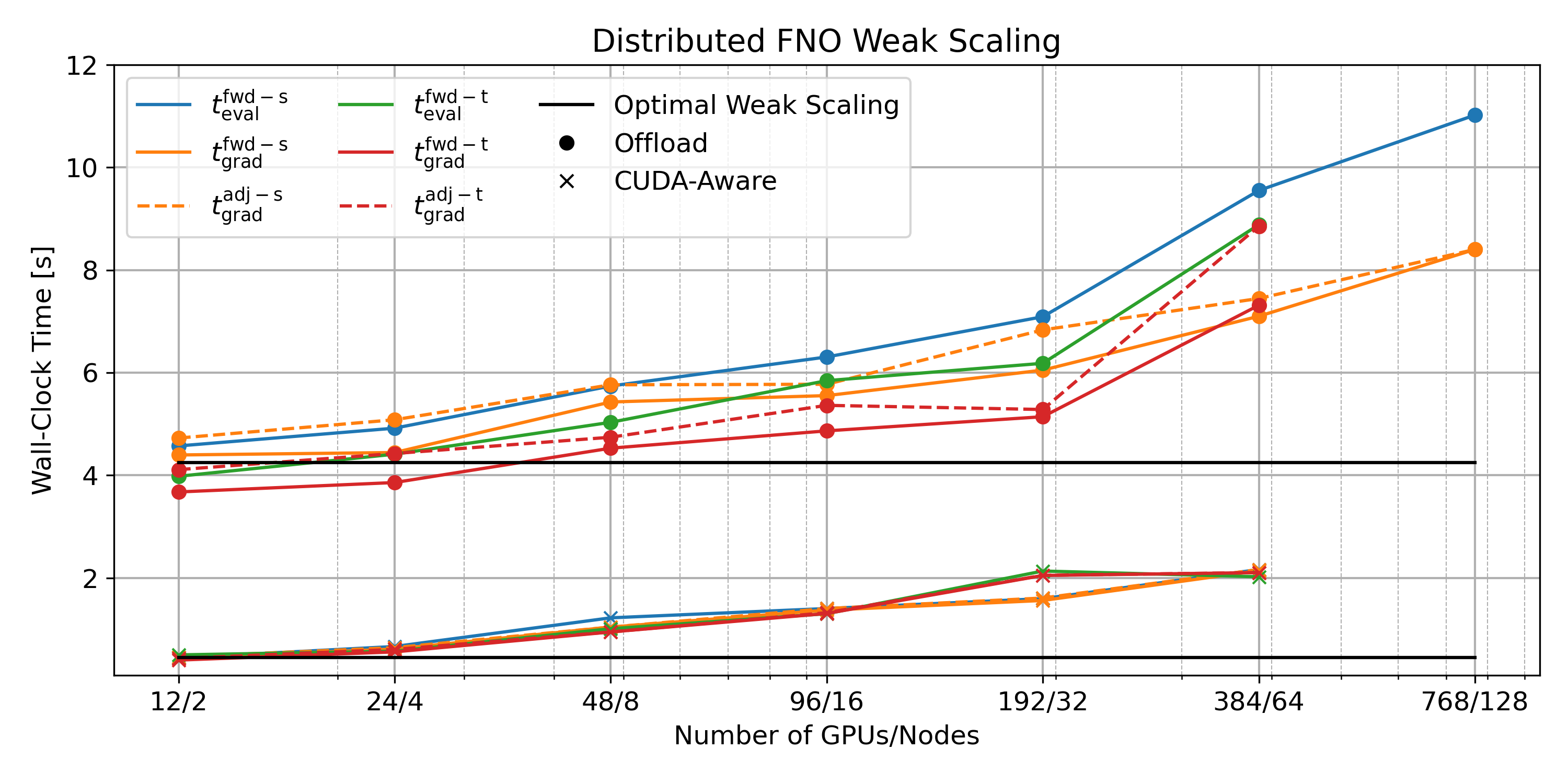
We demonstrate the scaling capabilities of our network on GPU nodes via a weak scaling study performed on the Summit supercomputer system at Oak Ridge National Laboratory. A plot of the results is shown in Figure 9 below. Overall, the network performs well for a complex all-to-all program, and allows for training on realistic datasets.
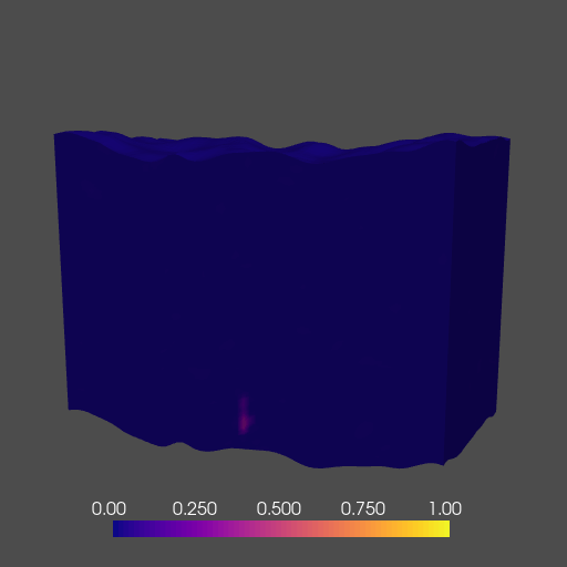
To demonstrate the abilities of our network, we train an FNO to act as a numerical surrogate to the solution(s) of the 3D time-varying two-phase flow equations. We model the behavior of subsurface CO2 on a class of models derived from an initial base rock physics model with added topographic (i.e. columnwise vertical displacement) perturbation. Our network runs during training and inference across multiple GPUs, and accurately predicts the complex behavior of two-phase flow in a fraction of the time of a traditional solver. A cross-section of the 3D solution is shown below in Figure 10.
References
Dalcin, L., Mortensen, M., and Keyes, D. E., 2018, Fast parallel multidimensional fFT using advanced mPI:. arXiv. doi:10.48550/ARXIV.1804.09536
Goodfellow, I., Pouget-Abadie, J., Mirza, M., Xu, B., Warde-Farley, D., Ozair, S., … Bengio, Y., 2014, Generative Adversarial Nets: In Proceedings of the 27th international conference on neural information processing systems (pp. 2672–2680). Retrieved from http://papers.nips.cc/paper/5423-generative-adversarial-nets.pdf
Hauptmann, A., Lucka, F., Betcke, M., Huynh, N., Adler, J., Cox, B., … Arridge, S., 2018, Model-based learning for accelerated, limited-view 3-d photoacoustic tomography: IEEE Transactions on Medical Imaging, 37, 1382–1393.
Hewett, R. J., Grady, T. J., and Merizian, J., 2021, Parallel primitives for domain decomposition in neural networks: Preprint. Under Review.
Hewett, R. J., Grady, T., and Merizian, J., 2021, Distdl/distdl: Version 0.4.0 release (Version v0.4.0). Zenodo. doi:10.5281/zenodo.5360401
Isola, P., Zhu, J.-Y., Zhou, T., and Efros, A. A., 2017, Image-to-Image Translation with Conditional Adversarial Networks: In The iEEE conference on computer vision and pattern recognition (cVPR) (pp. 5967–5976). doi:10.1109/CVPR.2017.632
Li, Z., Kovachki, N., Azizzadenesheli, K., Liu, B., Bhattacharya, K., Stuart, A., and Anandkumar, A., 2020, Fourier neural operator for parametric partial differential equations:. arXiv. doi:10.48550/ARXIV.2010.08895
Mao, X., Li, Q., Xie, H., Lau, R. Y., Wang, Z., and Paul Smolley, S., 2017, Least squares generative adversarial networks: In Proceedings of the iEEE international conference on computer vision (pp. 2794–2802).
Putzky, P., Karkalousos, D., Teuwen, J., Miriakov, N., Bakker, B., Caan, M., and Welling, M., 2019, I-rIM applied to the fastMRI challenge: ArXiv Preprint ArXiv:1910.08952.
Siahkoohi, A., Kumar, R., and Herrmann, F. J., 2019a, Deep-learning based ocean bottom seismic wavefield recovery: SEG technical program expanded abstracts. doi:10.1190/segam2019-3216632.1
Siahkoohi, A., Verschuur, D. J., and Herrmann, F. J., 2019b, Surface-related multiple elimination with deep learning: SEG technical program expanded abstracts. doi:10.1190/segam2019-3216723.1
Witte, P., Rizzuti, G., Louboutin, M., Siahkoohi, A., and Herrmann, F., 2020, InvertibleNetworks. jl: A julia framework for invertible neural networks:. November.
Zhang, M., Siahkoohi, A., and Herrmann, F. J., 2020, Transfer learning in large-scale ocean bottom seismic wavefield reconstruction: SEG technical program expanded abstracts. doi:10.1190/segam2020-3427882.1