Imaging

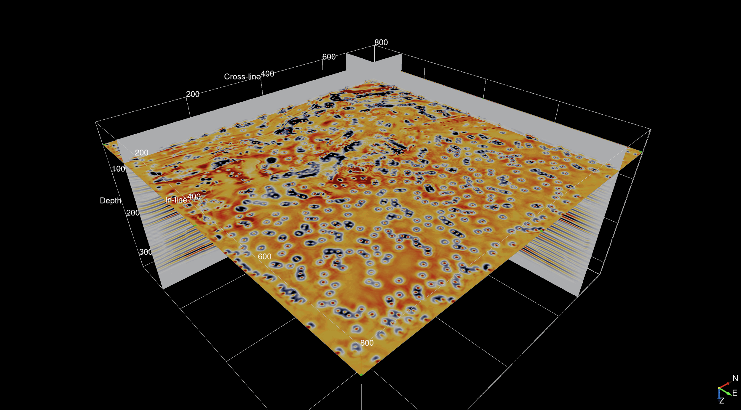
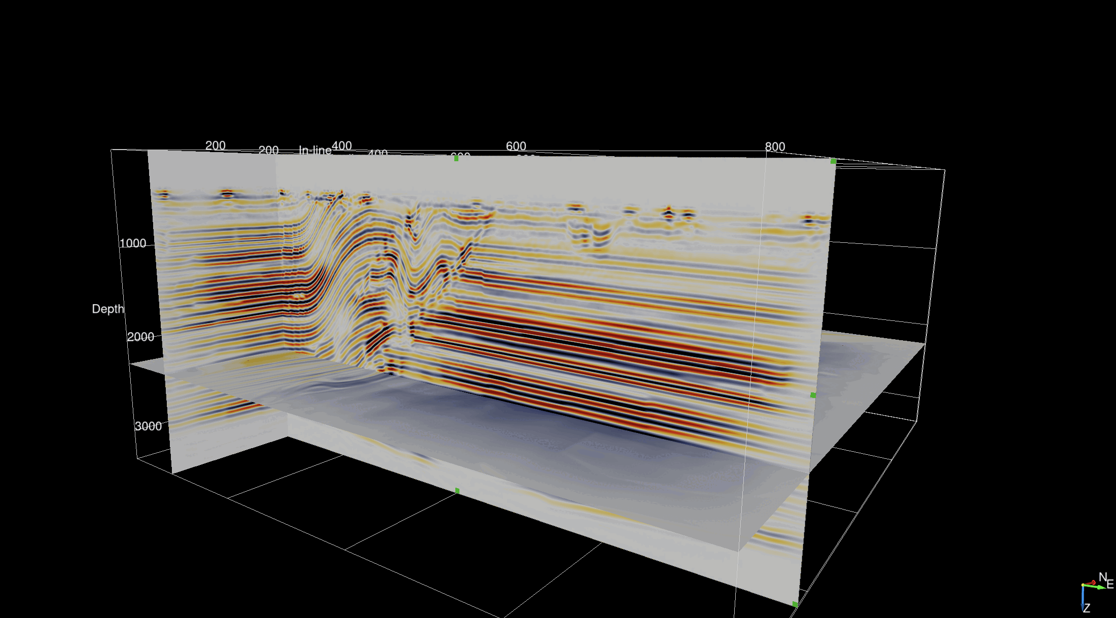
3D TTI reverse-time migration example

Introduction

At SLIM, we develop algorithms for high-fidelity subsurface and medical imaging for both standard and time-lapse imaging. Our research focuses on transform-domain structure promotion, scalability and multi-physics workflows using standard wave-equation based methods and machine learning. More specifically, we are actively working on

• Sparsity-promoting least-squares migration (Tu et al., 2013, 2016; Witte et al., 2019b; Daskalakis et al., 2020; Yang et al., 2020)
• Randomized linear algebra for seismic imaging (Louboutin and Herrmann, 2021, 2022)
• Time-lapse imaging for Geological Carbon Storage
• Seismic imaging with extensions (Yang et al., 2021)

Least-squares Reverse-Time Migration

Least-squares migration identifies the acquired seismic data as an approximate linear response to perturbations in the subsurface medium properties w.r.t. a smooth background (velocity model). By inverting the so-called “de-migration” or linearized Born scattering operator, which models linearized wave propagation, these medium perturbations that form the seismic image can be inverted for without the need to “relinearize”. Compared to conventional Reverse-Time Migration (RTM), the least-squares approach offers several benefits: (i) higher spatial resolution and true-amplitude fidelity as the illumination function (Gauss-Newton Hessian) and source signature(s) are deconvolved during the inversion (Tu et al., 2013); (ii) less acquisition footprints as the inversion procedure also accounts for the source illuminations (Nemeth et al., 1999); (iii) imaging with on-the-fly source estimation in the frequency (Tu et al., 2016) and time-domain (Yang et al., 2020); (iv) handling of surface-related multiples during imaging and (v) Compressive imaging with On-the-fly DFTs both of which are challenging with conventional RTM (Tu and Herrmann, 2014).

Given the source signature, \(\mathbf{q}_j\), least-squares migration involves \[ \begin{equation} \underset{{\delta\mathbf{m}}}{\operatorname{minimize}} \quad \sum_{j=i}^{n_s}\ \|\mathbf{d}_{j}-\nabla\mathbf{F}[\mathbf{m}_0,\mathbf{q}_j]\delta\mathbf{m}\|_2^2, \label{eq:1} \end{equation} \] where \(j\) is the sources index, \(n_s\) the number of source experiments, \(\nabla\mathbf{F}\) is the linearized Born scattering operator (Jacobian of Full-Waveform Inversion (FWI)), \(\mathbf{m}_0\) is the background model, \(\mathbf{q}_j\) is \(j\)th source signature, and \(\delta\mathbf{m}\) the unknown model perturbation to be inverted for.

One of the main challenges with least-squares reverse-time migration is the excessive computational cost. Each gradient update involves three wave-equation solves for each source experiment. This means that the total simulation cost is proportional to the number of sources in the inversion. Early work dimensionality reduction and stochastic optimization (Leeuwen et al., 2011; Haber et al., 2012; Aravkin et al., 2012) showed that randomized methods applied to the source sampling can lead to drastic cost reductions (factors of up to \(7\times\) have been reported by industry for FWI) while maintaining high accuracy. Current research focuses on the use of randomized methods to reduce the computational cost and memory footprint of wave-equation solves for each single source experiment. This will allow us to port the next-generation of least-square migration to accelerators such as GPUs.

Sparsity-promoting least-squares RTM

Following ideas on sparsity promotion from Compressive Sensing (CS) (Donoho, 2006; Candès et al., 2006) and from sparse Kaczmarz, linearized Bregman (Lorenz et al., 2014), and Accelerating sparse recovery by reducing chatter, (Daskalakis et al., 2020), we solve the following strongly convex optimization problem: \[ \begin{equation} \begin{aligned} &\min_{\mathbf{x}} \lambda \|\mathbf{x}\|_{\mathrm{1}} + \frac{1}{2} \|\mathbf{x}\|^2_{\mathrm{2}}\\ &\mathrm{subject\ to} \sum_{j=1}^{n_s} \|\mathbf{d}_{j}-\nabla\mathbf{F}[\mathbf{m}_0,\mathbf{q}_j]\mathbf{C}^\top\mathbf{x}\|_2^2 \leq\mathrm{\sigma} \end{aligned} \label{eq:elastic} \end{equation} \] via linearized Bregman iterations \[ \begin{equation} \begin{aligned} \begin{array}{lcl} \mathbf{z}_{k+1} & = & \mathbf{z}_k-t_k \mathbf{A}_k^\top(\mathbf{A}_k\mathbf{x}_{k}-\mathbf{b}_k)\\ \mathbf{x}_{k+1} & = & \mathbf{C}^\top S_{\lambda}(\mathbf{C}\mathbf{z}_{k+1}), \end{array} \end{aligned} \label{LBk} \end{equation} \] where the pair \(\{\mathbf{A}_k, \,\mathbf{b}_k\}\) represents (randomly without replacement) chosen subsets (with cardinality \(\ll n_s\)) of source experiments selected from \(\nabla\mathbf{F}[\mathbf{m}_0,\mathbf{q}_j],\, j=1\cdots n_s\) and the corresponding shot records \(\mathbf{b}_k\) extracted from \(\mathbf{d}_j,\, j=1\cdots n_s\). For properly selected steplengths, \(t_k\), and \(\lambda\) for the curvelet domain thresholding, the above iterations converge to the solution of problem \(\ref{eq:elastic}\). As we will show, problem \(\ref{eq:elastic}\) is conducive to accelerated and low-memory footprint sparsity-promoting inversion capable of producing high-fidelity true-amplitudes images at the cost of 2—3 conventional RTMs. After initializing the image and setting the source function, \(\mathbf{q}\), and the threshold, \(\lambda\), the Bregman iterations to solve our Sparsity-Promoting Least-Squares Reverse-Time Migration (SPLS-RTM) proceed as outlined in Algorithm 1 below.

Compressive imaging

While Sparsity-promoting least-squares RTM is a powerful approach for true-amplitude seismic imaging of complex geological structures, its successful application is hindered by its computational cost, as well as high memory requirements for computing gradients of the objective function. At SLIM, we have and continue to work on addressing these challenges by reducing the computations costs to \(2-3 \times\) the cost of RTM while drastically reducing the memory footprint so that the latest GPUs can be exploited. Below, we list some recent developments.

On-the-fly DFTs

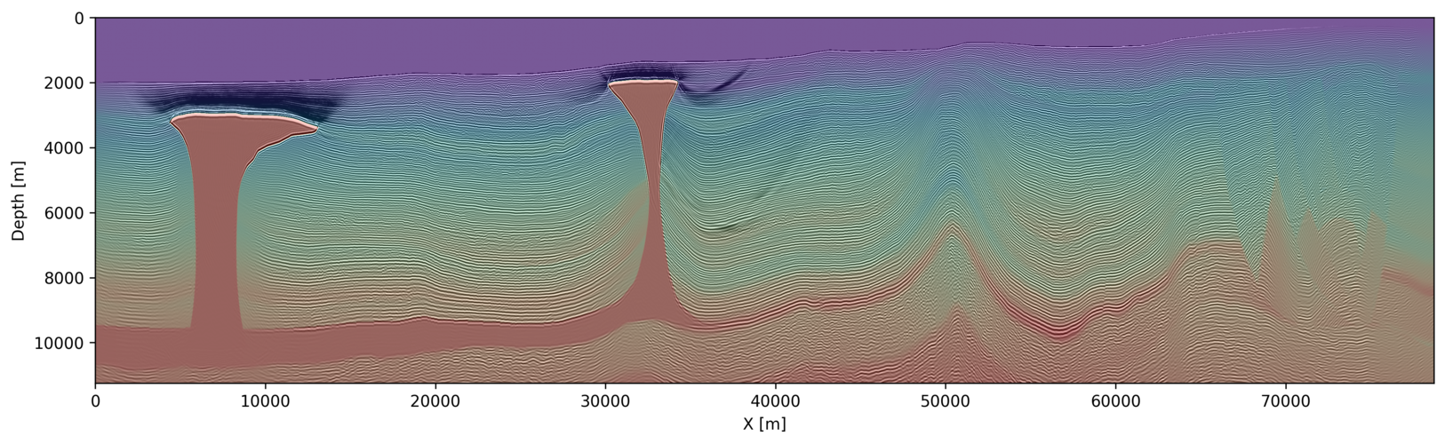
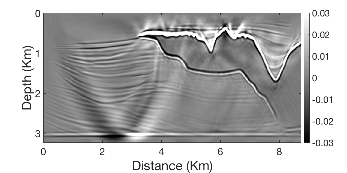
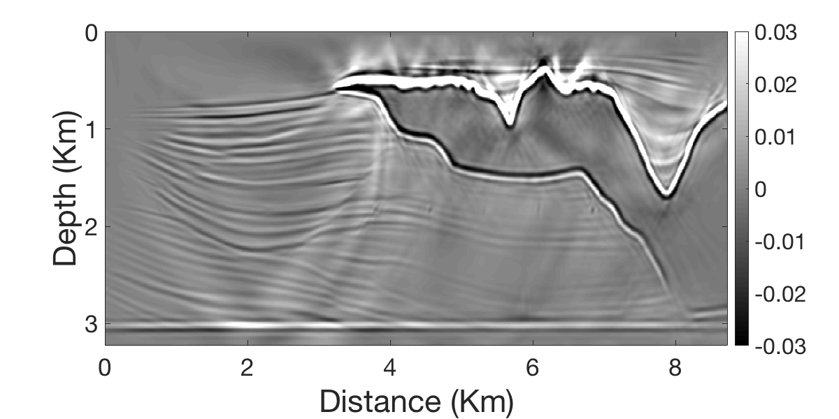
We tackle the computational challenges of Sparsity-promoting least-squares RTM (SPLS-RTM) by using on-the-fly Fourier transforms (Witte et al., 2019b). To this end, we approximate the least-squares migration objective in the frequency domain and compute gradients for randomized subsets of shot records, to reduce computational costs, and frequencies, to reduce memory pressure. With the on-the-fly Fourier transform, we have control over accuracy versus memory footprint by choosing the number of monochromatic time-harmonic wavefields that are computed with our highly-optimized time-domain finite-difference Modeling codes, implemented within our Julia Devito Inversion Framework JUDI (Witte et al., 2019b, 2019a). Figure #fig:2 below illustrates the performance of SPLS-RTM on the BP 2004 dataset. These results were obtained with significantly reduced memory footprint at the computational cost of \(3\times\) RTM.

Randomized trace estimation

While On-the-fly DFTs allow for reduction of memory, it requires complex arithmetic and can lead to coherent artifacts limiting achievable memory-footprint gains. To arrive at a simpler algorithm, we make use of recent results from the field of randomized linear algebra, a technique that has been shown to be a computationally efficient alternative to exact methods in exploration geophysics while conserving high accuracy, and in some cases providing access to information inaccessible via traditional methods. Examples of these methods are randomized SVD (Yang et al., 2021) applied to full subsurface-offset image volumes, and random phase encoding (Haber et al., 2012; Leeuwen et al., 2011) to reduce the working set of source experiments during seismic imaging and FWI.

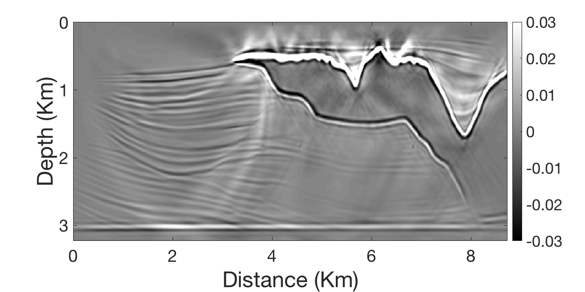
By using techniques from randomized trace estimation (Avron and Toledo, 2011; Persson et al., 2022), which also undergird our work on dimensionality reduction and stochastic optimization for seismic imaging and inversion, we approximate the gradient calculations for RTM and FWI by approximating the trace (sum of the diagonal of a matrix) of the outer product of the forward and adjoint wavefield with respect to time (Louboutin and Herrmann, 2021, 2022). As a result, the gradient calculations can be approximated via \[ \begin{equation} \delta\mathbf{m} = \sum_t \mathbf{\ddot{u}}[t] \mathbf{v}[t] = \operatorname{tr}\left(\mathbf{\ddot{u}}[t, \mathbf{x}]\mathbf{v}[t, \mathbf{x}]^\top\right) \approx \frac{1}{r} \operatorname{tr}\left((\mathbf{Q}^\top \mathbf{\ddot{u}}[\mathbf{x}]) (\mathbf{v}[\mathbf{x}]^\top \mathbf{Q})\right) \label{trace} \end{equation} \] where \(\mathbf{Q}\) is a carefully chosen matrix of probing vectors (Louboutin and Herrmann, 2021). Aside from being simpler, this approach performs better than On-the-fly DFTs. Figure 2 below shows an example of applying this technique on the BP 2007 TTI dataset. See FWI for the application of this technique to 3D. Its implementation using Devito and JUDI and additional examples can be found at TimeProbeSeismic.

Chatter reduction

Despite gains made in reducing the computational costs and memory footprint of SPLS-RTM, challenges remain related to the nonlinear phenomenon of chatter (Daskalakis et al., 2020), which stalls convergence of sparsity-promoting optimization with stochastic optimization during which stochasticity is injected during the iterations due selecting different subsets of (simultaneous) shots or due to approximations of the gradients via On-the-fly DFTs or Randomized trace estimation. Figure 3} contains an example of chatter where linearized Bregman iterations flip-flop between two different solutions.

By controlling chatter with weighted increments, which keep track of sign changes for each entry of the gradient vector (see Daskalakis et al. (2020) for detail), we are able to reduce the impact of chatter improving the inverted result.

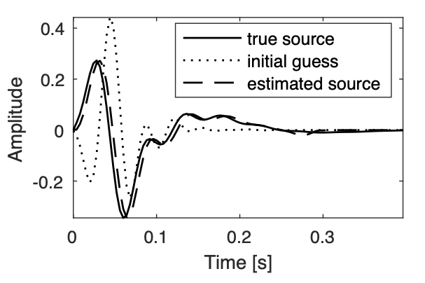
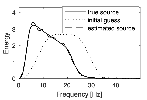
Time-domain source estimation

So far, we dealt with the computational aspects of SPLS-RTM while assuming we had access to the source signatures. In practice, we do not have access to this information. To address this issue, we extended earlier work on time-harmonic [On-the-fly source estimation] to the time domain by extending Algorithm 1 to include estimation of the source signature \(\mathbf{w}\) on line 10 in Algorithm 2 below.

For additional imaging work, check

• Monitoring for Time-lapse seismic and Geological Carbon Storage
• Extended imaging for imaging migration-velocity analysis, and velocity continuation with subsurface-offset image volumes
• Uncertainty-aware imaging for uncertainty quantification
• Imaging with tasks for propagating uncertainty from shot data to the horizon tracking in the image space
• Medical imaging wave-based inversion and uncertainty quantification

References

Aravkin, A. Y., Friedlander, M. P., Herrmann, F. J., and Leeuwen, T. van, 2012, Robust Inversion, Dimensionality Reduction, and Randomized Sampling: Mathematical Programming, 134, 101–125. doi:10.1007/s10107-012-0571-6
Avron, H., and Toledo, S., 2011, Randomized algorithms for estimating the trace of an implicit symmetric positive semi-definite matrix: Journal of the ACM (JACM), 58, 1–34.
Candès, E. J., Romberg, J. K., and Tao, T., 2006, Stable signal recovery from incomplete and inaccurate measurements: Communications on Pure and Applied Mathematics, 59, 1207–1223. doi:10.1002/cpa.20124
Daskalakis, E., Herrmann, F. J., and Kuske, R., 2020, Accelerating sparse recovery by reducing chatter: SIAM Journal on Imaging Sciences, 13, 12111239. doi:10.1137/19M129111X
Donoho, D., 2006, Compressed sensing: Information Theory, IEEE Transactions on, 52, 1289–1306. doi:10.1109/TIT.2006.871582
Haber, E., Chung, M., and Herrmann, F., 2012, An effective method for parameter estimation with pDE constraints with multiple right-hand sides: SIAM Journal on Optimization, 22, 739–757.
Leeuwen, T. van, Aravkin, A. Y., and Herrmann, F. J., 2011, Seismic waveform inversion by stochastic optimization: International Journal of Geophysics, 2011.
Lorenz, D. A., Wenger, S., Schöpfer, F., and Magnor, M., 2014, A sparse kaczmarz solver and a linearized bregman method for online compressed sensing: In 2014 iEEE international conference on image processing (iCIP) (pp. 1347–1351). doi:10.1109/ICIP.2014.7025269
Louboutin, M., and Herrmann, F., 2022, Enabling wave-based inversion on gPUs with randomized trace estimation: In 83rd eAGE annual conference & exhibition (Vol. 2022, pp. 1–5). European Association of Geoscientists & Engineers.
Louboutin, M., and Herrmann, F. J., 2021, Ultra-low memory seismic inversion with randomized trace estimation: SEG technical program expanded abstracts. doi:10.1190/segam2021-3584072.1
Nemeth, T., Wu, C., and Schuster, G. T., 1999, Least-squares migration of incomplete reflection data: Geophysics, 64, 208–221.
Persson, D., Cortinovis, A., and Kressner, D., 2022, Improved variants of the hutch++ algorithm for trace estimation: SIAM Journal on Matrix Analysis and Applications, 43, 1162–1185.
Tu, N., and Herrmann, F. J., 2014, Fast imaging with surface-related multiples by sparse inversion: UBC; UBC. Retrieved from https://slim.gatech.edu/Publications/Public/Journals/GeophysicalJournalInternational/2014/tu2014fis/tu2014fis.pdf
Tu, N., Aravkin, A. Y., Leeuwen, T. van, Lin, T. T., and Herrmann, F. J., 2016, Source estimation with surface-related multiples-fast ambiguity-resolved seismic imaging: Geophysical Journal International, 205, 1492–1511. Retrieved from https://slim.gatech.edu/Publications/Public/Journals/GeophysicalJournalInternational/2016/tu2015GJIsem/tu2015GJIsem.pdf
Tu, N., Li, X., and Herrmann, F. J., 2013, Controlling linearization errors in \(\ell_1\) regularized inversion by rerandomization: SEG technical program expanded abstracts. SEG. doi:10.1190/segam2013-1302.1
Witte, P. A., Louboutin, M., Kukreja, N., Luporini, F., Lange, M., Gorman, G. J., and Herrmann, F. J., 2019a, A large-scale framework for symbolic implementations of seismic inversion algorithms in julia: GEOPHYSICS, 84, F57–F71. doi:10.1190/geo2018-0174.1
Witte, P. A., Louboutin, M., Luporini, F., Gorman, G. J., and Herrmann, F. J., 2019b, Compressive least-squares migration with on-the-fly fourier transforms: Geophysics, 84, R655–R672. doi:10.1190/geo2018-0490.1
Yang, M., Fang, Z., Witte, P. A., and Herrmann, F. J., 2020, Time-domain sparsity promoting least-squares reverse time migration with source estimation: Geophysical Prospecting, 68, 2697–2711. doi:10.1111/1365-2478.13021
Yang, M., Graff, M., Kumar, R., and Herrmann, F. J., 2021, Low-rank representation of omnidirectional subsurface extended image volumes: Geophysics, 86, S165–S183.