
Extended imaging
Introduction
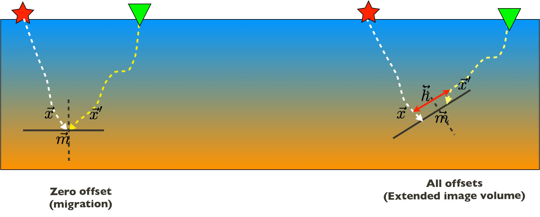
The formation of subsurface-offset gathers, such as common-image gathers (CIGs) (Rickett and Sava, 2002; W. W. Symes, 2008; Stolk et al., 2009; Kalita and Alkhalifah, 2016), angle-domain common-image gathers (ADCIGs) (de Bruin et al., 1990; Kumar et al., 2018), and common-image point gathers (CIPs) (P. Sava and Vasconcelos, 2011; Leeuwen and Herrmann, 2012) has become an essential component of modern seismic imaging workflows. Each gather provides crucial information on the velocity model and the scattering (amplitude versus offset). Contrary to CIGs, CIPs provide information on the complete scattering mechanism because they are functions of the full omni-directional subsurface offset (see Figure 1). Because of the high computational costs, subsurface-offset CIP gathers are often only evaluated at limited numbers of subsurface points and limited ranges of subsurface offsets. At SLIM, we overcome these limitations by offering a new perspective on image gathers by forming extended image volumes (EIVs, (Leeuwen et al., 2017a)), which are quadratic in the image size, as a function of all subsurface offsets for all subsurface points. We organize these EIVs in a matrix whose \((i,j)^{\mathrm{th}}\) entry captures the interaction between gridpoints \(i\) and \(j\). We then propose efficient ways to probe and factorize these EIVs providing us with information for all subsurface midpoints (\(\vec{m}\)) and offsets (\(\vec{h}\)) \[ \begin{equation} \vec{m}=\frac{\vec{x}+\vec{x}^\prime}{2}\quad \text{and}\quad \vec{h}=\frac{\vec{x}-\vec{x}^\prime}{2}, \label{eq:offset} \end{equation} \] without explicitly calculating the source and receiver wavefields for all sources.
Full subsurface extended image volumes
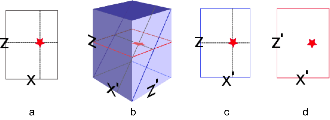
To arrive at our formulation, we arrange the time-harmonic source and receiver wavefields into the matrices \(U\) and \(V\), where each column corresponds to a source experiment. Given these matrices, the EIV at a single frequency, for all subsurface offsets and for all subsurface points can be written as the outer product between these two matrices, i.e., we have \[ \begin{equation} E = VU^*, \label{eq:E} \end{equation} \] where \(U,V\) are calculated using the two-way wave-equation. Figure 2 illustrates how the different subsurface-offset gathers are embedded in the 4-dimensional EIV.
In 2D, the EIVs are 5-dimensional functions of all subsurface offsets and temporal shifts. So even in this case, it is prohibitively expensive to compute and store the extended image for all the subsurface points. To overcome this problem, we select \(l\) columns of \(E\) implicitly by multiplying this matrix with the tall matrix \(W = [{\bf{w}}_1, \ldots, {\bf{w}}_{l}]\) yielding, \[ \begin{equation} \widetilde{E} = EW, \label{eq:EW} \end{equation} \] where \({\bf{w}}_i = [0, \ldots, 0, 1, 0,\ldots, 0]\) represents a single scattering point with the location of \(1\) corresponding to \(i^{th}\) grid location of the point scatterer. Now each column of \(\widetilde{E}\) represents a Common Image Point (CIP) gather at the locations represented by \({\bf{w}}_i\). We follow (Leeuwen and Herrmann, 2012) to efficiently compute \(\widetilde{E}\) by combining equations \(\ref{eq:E}\) and \(\ref{eq:EW}\) as \[ \begin{equation*} \widetilde{E} = EW = H^{-*}P_r^TDQ^*P_sH^{-*}W, \end{equation*} \] where \(H\) is a discretization of the Helmholtz operator \((\omega^2 \mathrm{diag}(\mathbf{m}) + \nabla^2)\) with \(\mathbf{m}\) the squared slowness and \(\nabla^2\) the Laplacian. The matrix \(Q\) represents the source function, \(*\) the conjugate-transpose, \(D\) is the data matrix and \(P_s, P_r\) sample the wavefield at the source and receiver positions (and hence, their transpose injects the sources and receivers into the grid). We can compute this product efficiently as follows:
- compute \(\widetilde{U} = H^{-*}W\) and sample this wavefield at the source locations \(\widetilde{D} = P_s\widetilde{U}\);
- correlate the result with source function \(\widetilde{Q} = Q^*\widetilde{D}\);
- use the result as data weights \(\widetilde{W} = D\widetilde{Q}\);
- inject the wavefield \(\widetilde{W}\) at the receiver locations and compute the extended image as \(\widetilde{E} = H^{-*}P_r^T\widetilde{W}\).
The computational cost of calculating \(\widetilde{E}\) is \(2l\) PDE solves plus the cost of correlating the source and data matrices. Thus, the cost of computing the CIPs does not depend on the number of sources or the number of subsurface offsets, as it does for conventional methods used to form CIG’s (Paul and Ivan, 2011). This is particularly beneficial when we are interested in computing only a few CIPs. An overview of the computational complexity is shown in Table 1.
| # of PDE solves | flops | |
|---|---|---|
| conventional | \(2 N_s\) | \(N_s N_{h_x} N_{h_y} N_{h_z}\) |
| this work | \(2 N_x\) | \(N_r N_s\) |
Below, we list a number of applications of EIVs.
AVA analysis and geological dip estimation
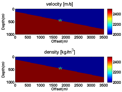
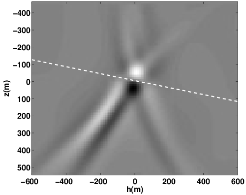
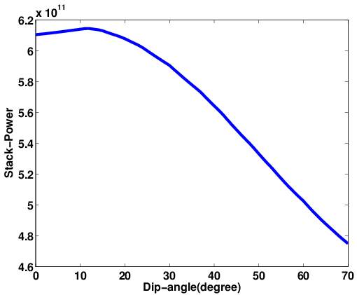
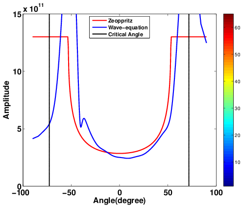
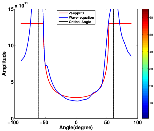
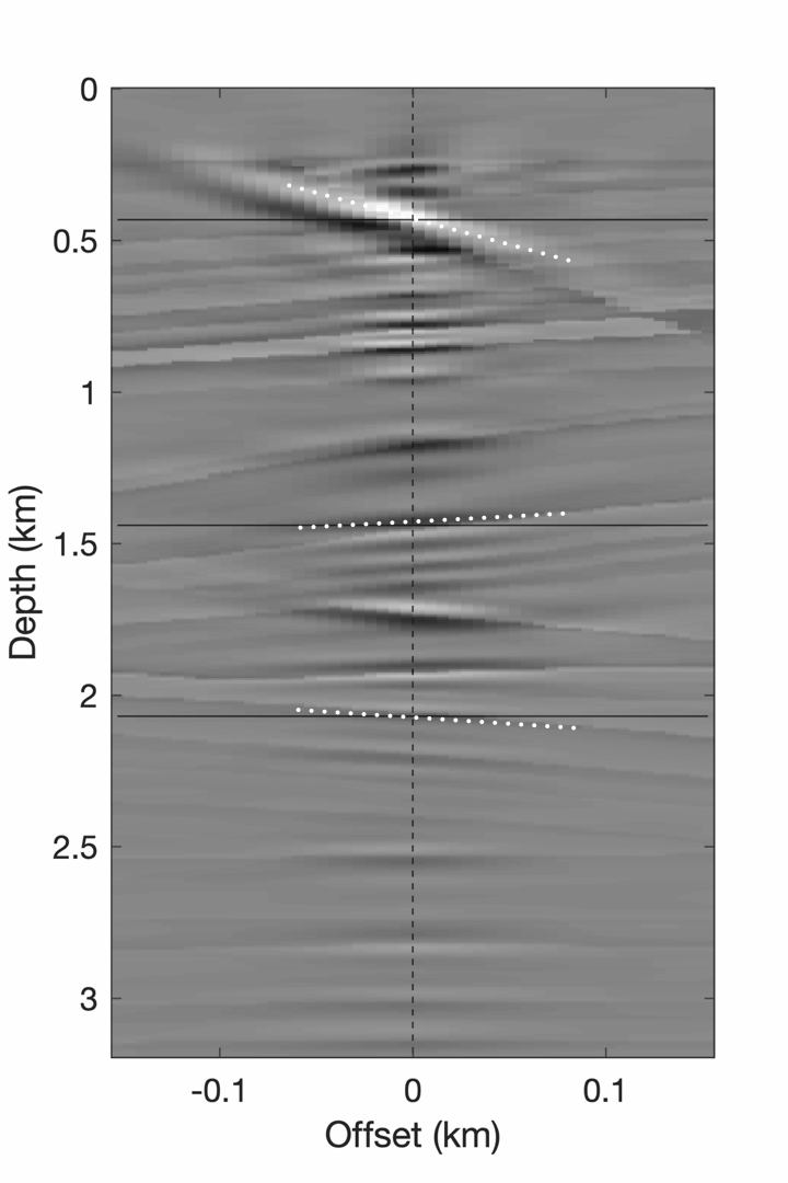
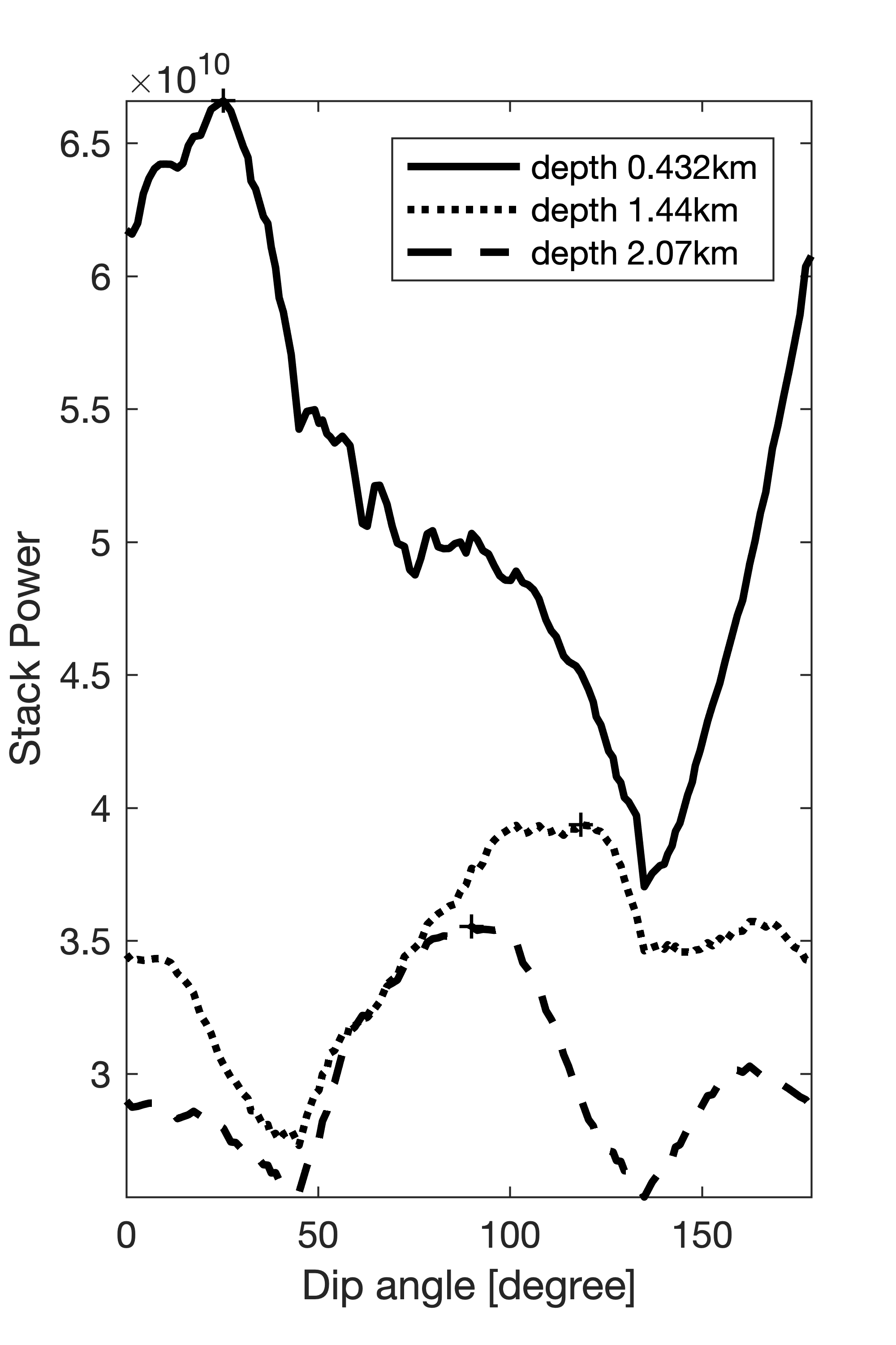
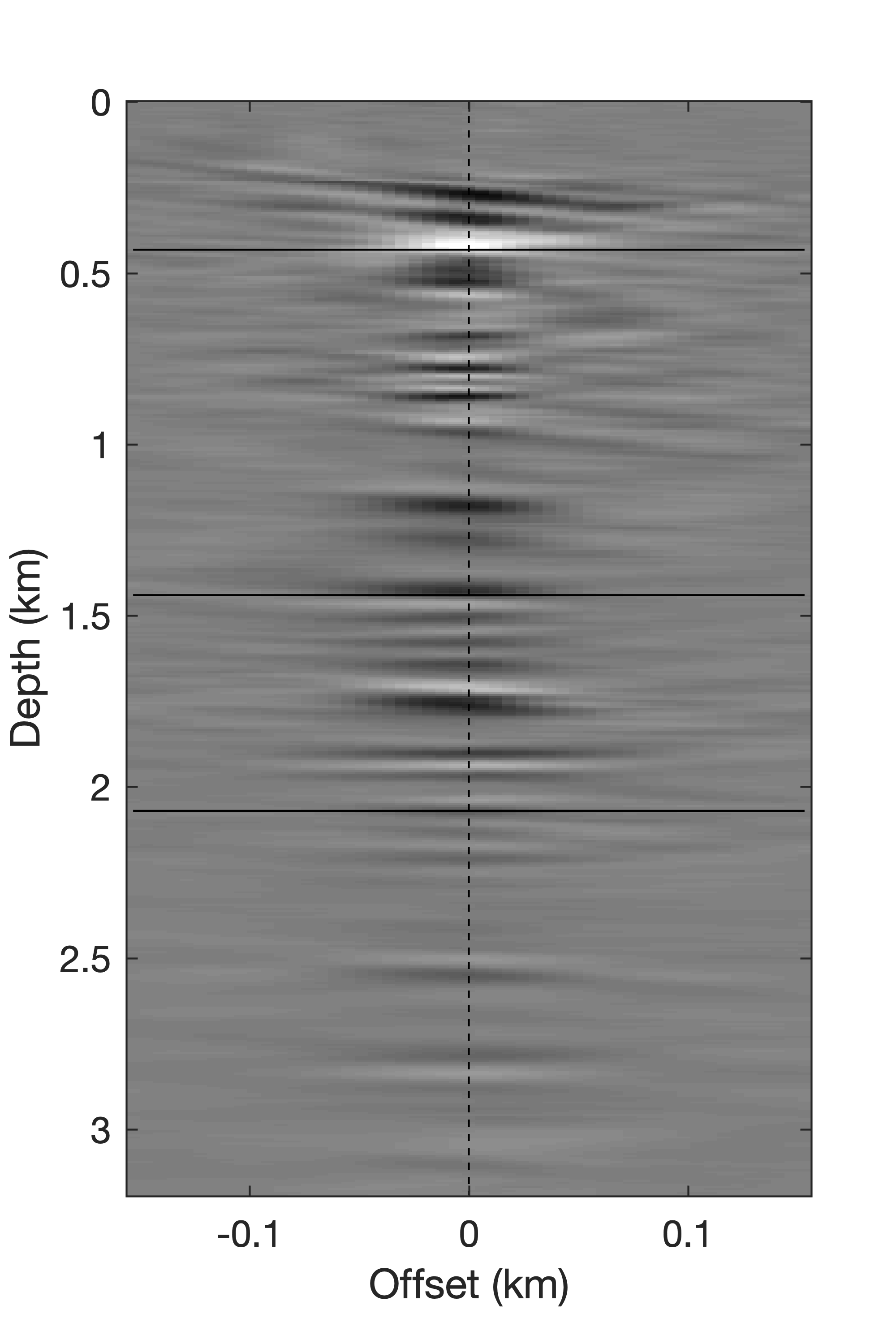
Because EIVs contain all possible subsurface offsets, its possible to correct angle-domain CIGs ofr the local geologic dip by selecting the appropriate subsurface offsets. To accomplish this, we do not need a priori information on local geological dip to perform AVA analysis. (Kumar et al., 2013; Leeuwen et al., 2017b) showed that local dip information can be computed on the fly from CIG’s. To assess the quality of the angle-domain common-image-points gathers, we compute the angle-dependent reflectivity coefficients and compare them with theoretical reflectivity coefficients yielded by the (linearized) Zoeppritz equations (Figure 3, 4). These Figures demonstrate that these dip corrections are feasible and can lead to significant improvements in the CIG’s as shown in Figure 5
Migration velocity analysis
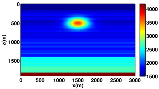
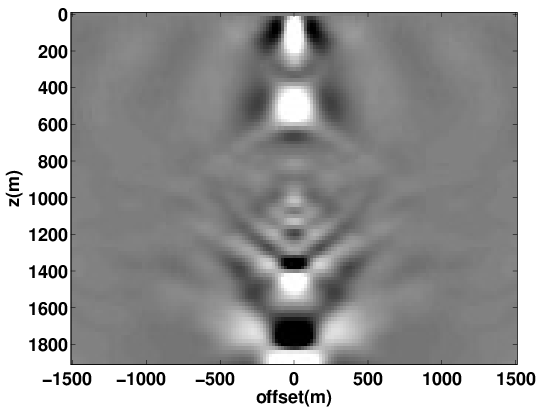
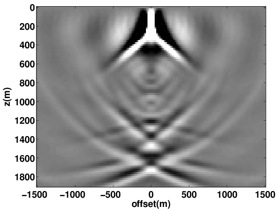
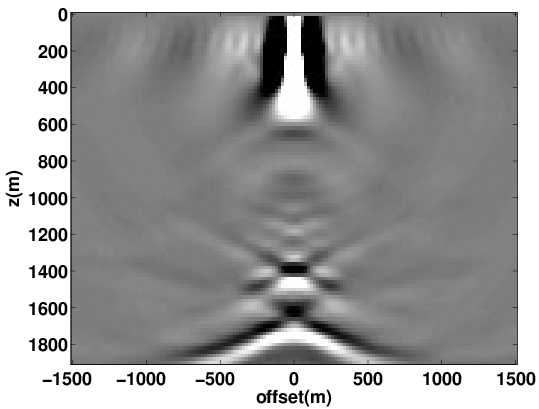
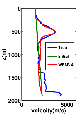
To achieve accurate high-fidelity images of the subsurface, estimation of the migration velocity model is crucial. Wave-equation based migration velocity analysis (WEMVA) is one such tool for velocity estimation in complex geological settings. The objective of WEMVA is to measure the focusing of common-image gathers (CIGs) by formulating an appropriate cost function (Biondi and Symes, 2004; Shen and Symes, 2008; W. W. Symes, 2008; P. Sava and Vasconcelos, 2011). In order to perform the automatic MVA, (Shen and Symes, 2008) considered penalizing the extended images as a function of subsurface offset with lateral shifts, which in our formulation is equivalent to demanding that our EIV matrix commutes with point-wise multiplication with the \(\bf{x}\)-position. For a focused image (Leeuwen et al., 2017b), we want to enforce that \[ \begin{equation*} E\mathrm{diag}({\bf{x}}) \approx \mathrm{diag}({\bf{x}})E. \end{equation*} \] The obvious way to achieve this is by formulating the optimization problem as \[ \begin{equation*} \min_{\bf{m}} \phi({\bf{m}}) = ||E({\bf{m}})\mathrm{diag}({\bf{x}}) - \mathrm{diag}({\bf{x}})E({\bf{m}})||^2, \end{equation*} \] where \(\| . \|\) is a matrix norm. If we choose the Frobenius norm as the matrix norm, then we can estimate this penalty via randomized trace estimation without explicitly forming the whole matrix as shown in (Kumar et al., 2014; Leeuwen et al., 2017b). Figure 6 shows the experimental results using proposed WEMVA formulation on Lens model.
Low-rank factorization
While the formation of EIVs allowed for new and enabling perspectives on seismic imaging, migration velocity analyses, and redatuming (Kumar et al., 2019) computational challenges remained. To address these, Yang et al. (2021) proposed a low-rank factorizing for EIVs based on randomized SVDs. This LR factorization provides access to the migrated image, CIPs, and CIG all from these factors alone. Given the number of probing vectors \(n_p\) and \(q\), this randomized SVD involves the steps outlined in Algorithm 1.
0. Input: \(q\) and \(n_p\) random Gaussian vectors \(\mathbf{W}=[\mathbf{w}_1, \cdots, \mathbf{w}_{n_p}]\)
1. \(\mathbf{K} := [ \mathbf{E}\mathbf{W}, (\mathbf{E}\mathbf{E}^*)\mathbf{E}\mathbf{W},\cdots, (\mathbf{E}\mathbf{E}^*)^q \mathbf{E}\mathbf{W} ], \mathbf{K} \in \mathbb{C}^{N \times (q+1) n_p}\)
2. \([\mathbf{Q},\sim]=\text{qr}(\mathbf{K}), \mathbf{Q} \in \mathbb{C}^{N \times (q+1) n_p}\)
3. \(\mathbf{Z}= \mathbf{E}^* \mathbf{Q} , \mathbf{Z} \in \mathbb{C}^{N \times (q+1) n_p}\)
4. \([\mathbf{\Phi}, \mathbf{\Sigma}, \mathbf{\Psi}]=\text{svd}(\mathbf{Z}^*)\), svd computes the top \(n_p\) singular vectors
5. set \(\mathbf{\Phi} \leftarrow \mathbf{Q} \mathbf{\Phi}\), \(\mathbf{Q}\) chooses the first \(n_p\) singular vectors
6. \(\mathbf{L} = \mathbf{\Phi}\sqrt{\mathbf{\Sigma}}, \mathbf{R}=\mathbf{\Psi}\sqrt{\mathbf{\Sigma}}\)
7. Output: factors \(\{\mathbf{L},\, \mathbf{R}\}\) yielding \(\mathbf{E}\approx \mathbf{L}\mathbf{R}^*\)
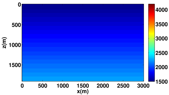
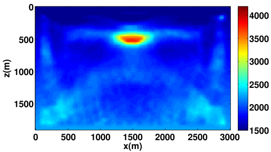
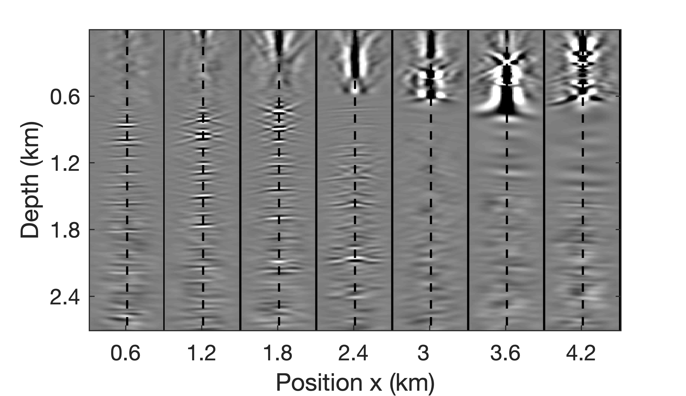
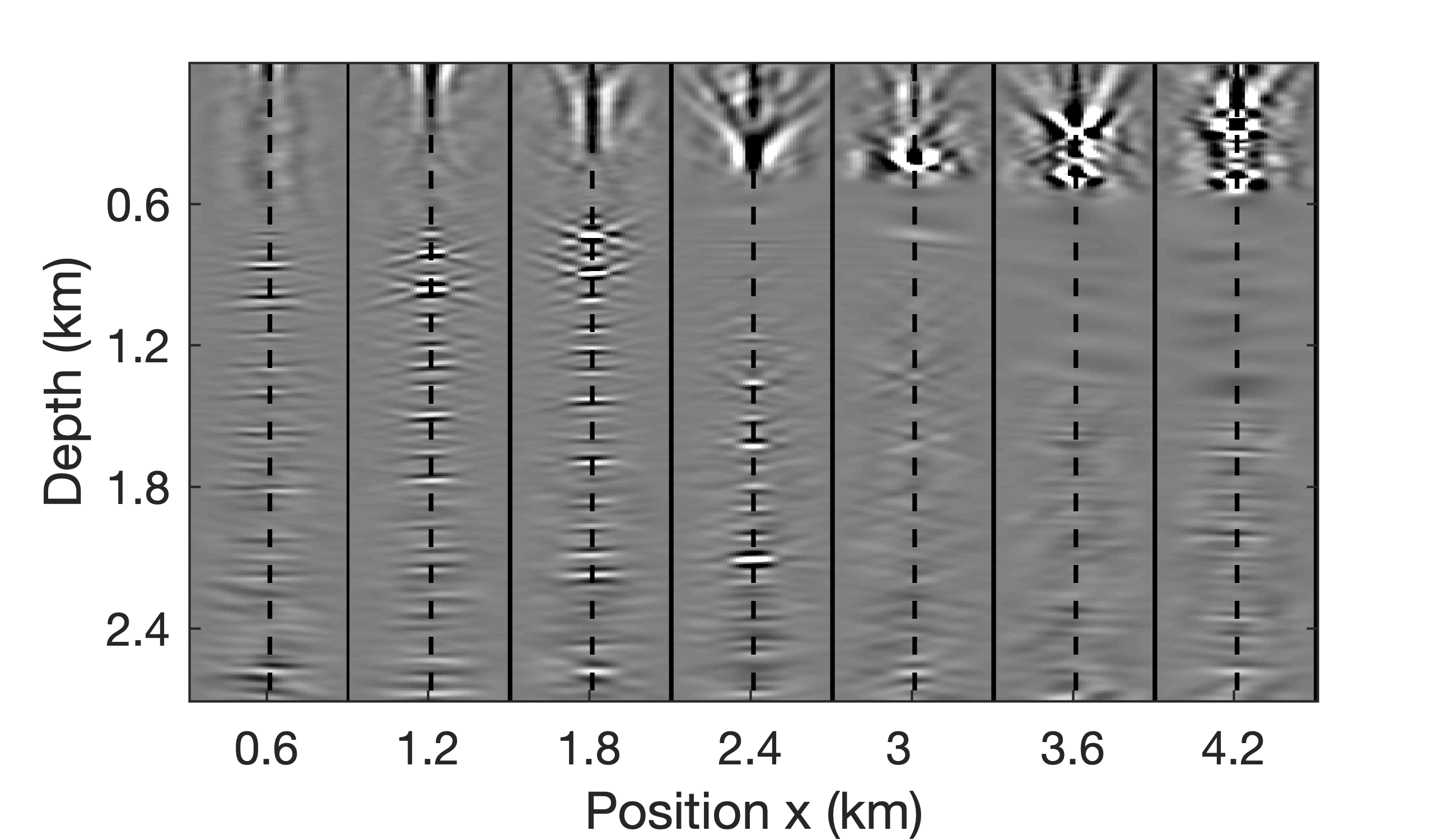
Velocity continuation
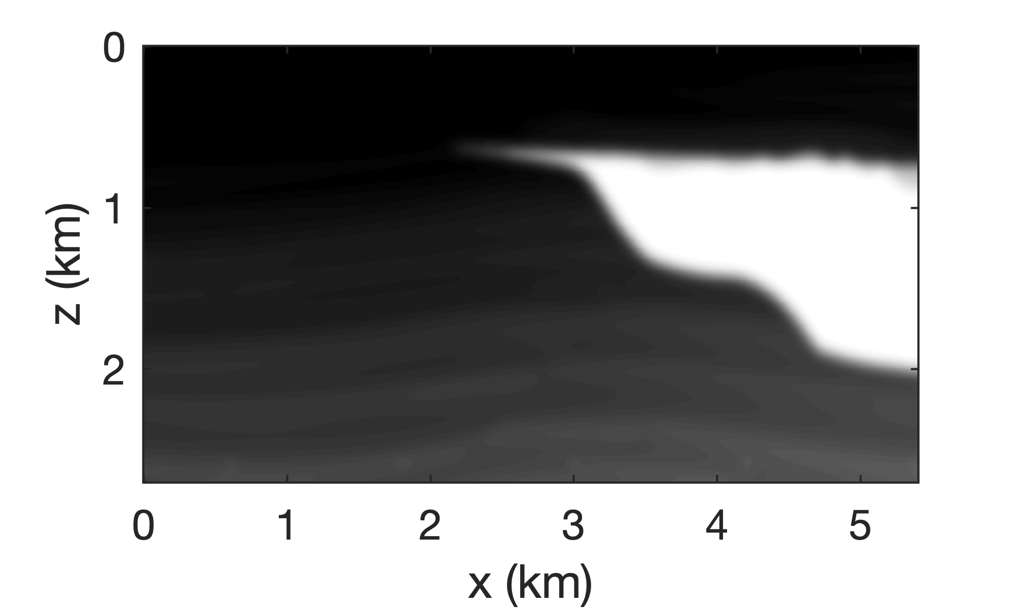
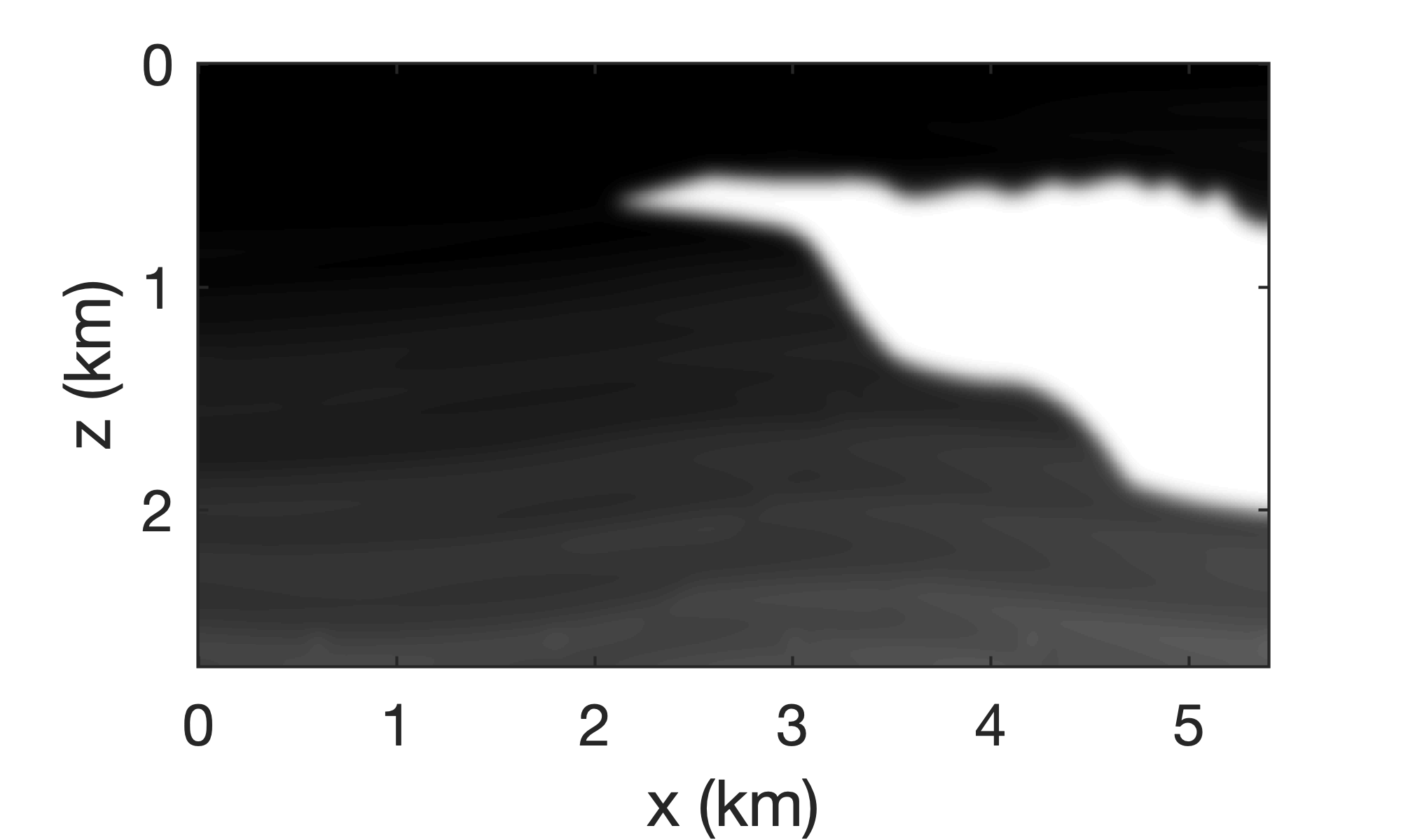
Given the L, R factorization, invariance-properties of EIVs (Kumar et al., 2019) can be used to map EIVs, or factors thereof, for one velocity model to another without the need to refactor—i.e., the factors for velocity model \(2\) can be related to these of velocity model \(1\) via \[ \begin{equation} \begin{aligned} \mathbf{L}_{2} &= \mathbf{H}_{2}^{-*} \cdot \mathbf{H}_{1}^{*} \cdot \mathbf{L}_{1}, \\ \\ \mathbf{R}_{2} &= \mathbf{H}_{2}^{-1} \cdot \mathbf{H}_{1} \cdot \mathbf{R}_{1}. \end{aligned} \label{eq:factors} \end{equation} \] involving fewer applications of the wave equation and its inverse (Yang et al., 2021). Based on these expressions, we are able to map the LR factors between the velocity models plotted in Figure 7. Given the new factors,
References
Biondi, B., and Symes, W. W., 2004, Angle-domain common-image gathers for migration velocity analysis by wavefield-continuation imaging: Geophysics, 69, 1283. Retrieved from http://sepwww.stanford.edu/sep/biondo/PDF/Journals/Geophysics/adcig-geo-online.pdf
de Bruin, C., Wapenaar, C., and Berkhout, A., 1990, Angle-dependent reflectivity by means of prestack migration: Geophysics, 55, 1223–1234.
Kalita, M., and Alkhalifah, T., 2016, Common-image gathers using the excitation amplitude imaging condition: GEOPHYSICS, 81, S261–S269. doi:10.1190/geo2015-0413.1
Kumar, R., Graff-Kray, M., Leeuwen, T. van, and Herrmann, F. J., 2018, Low-rank representation of extended image volumes––applications to imaging and velocity continuation: SEG technical program expanded abstracts. doi:10.1190/segam2018-2998404.1
Kumar, R., Graff-Kray, M., Vasconcelos, I., and Herrmann, F. J., 2019, Target-oriented imaging using extended image volumesa low-rank factorization approach: Geophysical Prospecting, 67, 1312–1328. doi:10.1111/1365-2478.12779
Kumar, R., Leeuwen, T. van, and Herrmann, F. J., 2013, AVA analysis and geological dip estimation via two-way wave-equation based extended images: SEG technical program expanded abstracts. SEG. Retrieved from https://slim.gatech.edu/Publications/Public/Conferences/SEG/2013/kumar2013SEGAVA/kumar2013SEGAVA.pdf
Kumar, R., Leeuwen, T. van, and Herrmann, F. J., 2014, Extended images in action: Efficient WEMVA via randomized probing: EAGE. Retrieved from http://www.earthdoc.org/publication/publicationdetails/?publication=76362
Leeuwen, T. van, and Herrmann, F. J., 2012, Wave-equation extended images: Computation and velocity continuation: EAGE technical program. EAGE. Retrieved from https://slim.gatech.edu/Publications/Public/Conferences/EAGE/2012/vanleeuwen2012EAGEext/vanleeuwen2012EAGEext.pdf
Leeuwen, T. van, Kumar, R., and Herrmann, F. J., 2017a, Enabling affordable omnidirectional subsurface extended image volumes via probing: Geophysical Prospecting, 65, 385–406. Journal Article. doi:https://doi.org/10.1111/1365-2478.12418
Leeuwen, T. van, Kumar, R., and Herrmann, F. J., 2017b, Enabling affordable omnidirectional subsurface extended image volumes via probing: Geophysical Prospecting, 65, 385–406. doi:10.1111/1365-2478.12418
Paul, S., and Ivan, V., 2011, Extended imaging conditions for wave-equation migration: Geophysical Prospecting, 59, 35–55. Retrieved from http://onlinelibrary.wiley.com/doi/10.1111/j.1365-2478.2010.00888.x/abstract
Rickett, J. E., and Sava, P. C., 2002, Offset and angle‐domain common image‐point gathers for shot‐profile migration: GEOPHYSICS, 67, 883–889. doi:10.1190/1.1484531
Sava, P., and Vasconcelos, I., 2011, Extended imaging conditions for wave-equation migration: Geophysical Prospecting, 59, 35–55. Retrieved from http://onlinelibrary.wiley.com/doi/10.1111/j.1365-2478.2010.00888.x/abstract
Shen, P., and Symes, W. W., 2008, Automatic velocity analysis via shot profile migration: Geophysics, 73, VE49–VE59. Retrieved from http://onlinelibrary.wiley.com/doi/10.1111/j.1365-2478.2010.00888.x/abstract
Stolk, C. C., Hoop, M. V. de, and Symes, W. W., 2009, Kinematics of shot-geophone migration: GEOPHYSICS, 74, WCA19–WCA34. doi:10.1190/1.3256285
Symes, W. W., 2008, Migration velocity analysis and waveform inversion: Geophysical Prospecting, 56, 765–790. Retrieved from http://www.trip.caam.rice.edu/reports/2007/amva2.pdf
Yang, M., Graff, M., Kumar, R., and Herrmann, F. J., 2021, Low-rank representation of omnidirectional subsurface extended image volumes: Geophysics, 86, 1MJ–WA152. doi:10.1190/geo2020-0152.1