High-frequency wavefield recovery with weighted matrix factorizations

Introduction

Seismic data acquisition is one of the key steps in initial phase of oil & gas exploration. Due to operational complexity and operational costs, acquired seismic data is usually not fully sampled, a prerequisite to subsequent steps such as multiple removal and migration all of which require densely sampled data.

Wavefield recovery is an important tool to solve the problem of poor sampling. In the last decade, wavefield recovery methods based on sparsity promotion in different transform domains, such as the Radon (Bardan, 1987), wavelet (Villasenor et al., 1996), and curvelet (Herrmann et al., 2007; Herrmann and Hennenfent, 2008) domain have been developed. Although these methods are valuable in terms of the quality of recovered data, they are relatively complex and computationally expensive. Fortunately, matrix completion methods (Kumar et al., 2015) based on low-rank matrix factorizations are relatively simple and computationally cheaper. The latter use the property that fully-sampled frequency slices permit accurate low-rank representations when organized in midpoint/offset. In Kumar et al. (2015); Oropeza and Sacchi (2011), authors exploit the fact that presence of noise or missing traces increases the rank of these frequency slices. We use this property to recover frequency slices via factored rank minimization (Kumar et al., 2014). While this matrix factorization method performs well at the low to mid frequencies, it struggles to recover high-frequency data, which need higher ranks to be accurately represented.

Recent work by A. Aravkin et al. (2014); Eftekhari et al. (2018) has shown that reliable prior information on the row and column subspaces of the underlying low rank matrix can be used to further improve wavefield recovery via matrix completion. For seismic data, we have access to this information when there is a strong similarity between adjacent frequency slices. In that case, the row and column subspaces can serve as prior information. This principle was first demonstrated by A. Aravkin et al. (2014) and we extend this line of research by recursively invoking prior as we work our way from the relatively low frequencies to the high frequencies where conventional matrix completion methods typically perform poorly.

We organize our paper as follows. First, we discuss wavefield recovery via matrix completion. Next, we discuss how to incorporate prior information on the row and column subspaces from neighboring lower frequencies in our matrix completion framework. We conclude demonstrating our approach on a field data example from the Gulf of Suez and show its better performance compared to conventional matrix completion especially at the higher frequencies.

Methodology

Low-rank matrix factorization

In Kumar et al. (2015) and A. Aravkin et al. (2014), authors exploit low rank of fully sampled seismic data by solving for each frequency problem of the type \[ \begin{equation} \minim_{\vector{X}_{i}} \quad \|\vector{X}_{i}\|_* \quad \text{subject to} \quad \|\mathcal{A}(\vector{X}_{i}) - \vector{b}_{i}\|_{2} \leq \epsilon. \label{eqBPDN} \end{equation} \] In this expression, the matrices \(\vector{X}_{i}\) for \(i=1\cdots n_f\) with \(n_f\) the number of angular frequencies represent fully sampled monochromatic frequency slices in the midpoint/offset domain, \(\mathcal{A}\) is the sampling operator collecting the data into a vector, and \(\vector{b}_i\) represents the observed data at the \({i}^{th}\) frequency. For each frequency, we recover the fully sampled data by minimizing the nuclear norm \(\|\cdot\|_*\) on each \(\vector{X}_{i}\) subject we fit the data within \(\epsilon\). The nuclear norm itself is defined as the sum of the singular values. We solve Equation \(\ref{eqBPDN}\) for all the frequencies to obtain our recovered data \(\vector{X} \in \mathbb{C}^{n_f \times n_m \times n_h}\), where \(n_m\) is the number of midpoints and \(n_h\) the number of offsets. As reported by Kumar et al. (2015), randomized sampling increases the rank of \(2\)D seismic data in midpoint offset domain, which is a favorable condition for matrix completion.

To avoid computationally expensive singular-value decompositions (SVD) while solving \(\ref{eqBPDN}\), we employ a low-rank matrix factorization approach. For this purpose, we factor the matrices (for notational simplicity we drop the subscript \(_i\)) \(\vector{X} \in \mathbb{C}^{n_m \times n_h}\) in Problem \(\ref{eqBPDN}\) into the low-rank factors \(\vector{L} \in \mathbb{C}^{n_m \times {r}}\) and \(\vector{R} \in \mathbb{C}^{n_h \times {r}}\) both of rank \({r}\). To avoid expensive SVDs, we follow Rennie and Srebro (2005) and replace the nuclear norm in Problem \(\ref{eqBPDN}\) by \[ \begin{equation} \begin{split} \minim_{\vector{L}, \vector{R}} \quad \frac{1}{2} {\left\| \begin{bmatrix} \vector{L} \\ \vector{R} \end{bmatrix} \right\|}_F^2 \quad \text{subject to} \quad \|\mathcal{A}(\vector{L}\vector{R}^{H}) - \vector{b}\|_{F} \leq \epsilon, \end{split} \label{eqSrcest} \end{equation} \] where \(^{H}\) is the Hermitian transpose and \(\|\cdot\|_F\) the Frobenius norm (2-norm of the vectorized matrix). Following Kumar et al. (2015) and A. Aravkin et al. (2014), we solve Problem \(\ref{eqSrcest}\) with spectral-projected gradients (Van Den Berg and Friedlander, 2008).

As we mentioned earlier, the performance of low-rank factorization methods degrade with increasing frequency reflected in increasing poor signal to noise ratios (SNRs) (Kumar et al., 2015). To improve the recovered data quality at higher frequencies, we include weighted matrix completion (A. Aravkin et al., 2014; Eftekhari et al., 2018).

Weighted low-rank matrix factorization

The key of our methodology is that we approximate fully sampled data in low-rank factored form. When using SVDs, this factored form reads \[ \begin{equation} \vector{X} \approx \vector{U}\Sigma\vector{V}^H, \label{eqsvd} \end{equation} \] where \(\vector{U} \in \mathbb{C}^{n_m \times r}\) and \(\vector{V} \in \mathbb{C}^{n_h \times r}\) are column and row subspaces of \(\vector{X}\), respectively. \(\Sigma \in \mathbb{C}^{{r} \times {r}}\) is a diagonal matrix containing the largest \(r\) singular values of the matrix \(\vector{X}\).

As shown by A. Aravkin et al. (2014); Eftekhari et al. (2018), information on these subspaces can be used to rewrite Problem \(\ref{eqBPDN}\) into its weighted form—i.e., we have \[ \begin{equation} \minim_{\vector{X}} \quad \|\vector{Q}\vector{X}\vector{W}\|_* \quad \text{subject to} \quad \|\mathcal{A}(\vector{X}) - \vector{b}\|_2 \leq \epsilon, \label{eqSrces} \end{equation} \] where \[ \begin{equation} \vector{Q} = {w}_{1}\vector{U}\vector{U}^H + \vector{U}^\perp \vector{U}^{{\perp}{H}} \label{eqprojl} \end{equation} \] and \[ \begin{equation} \vector{W} = {w}_{2}\vector{V}\vector{V}^H + \vector{V}^\perp \vector{V}^{{\perp}{H}} \label{eqprojr} \end{equation} \] are projection matrices on subspaces spanned by \(\vector{U}\), \(\vector{V}\) and their orthogonal complements \(\vector{U}^\perp\), \(\vector{V}^\perp\). The scalars \({w}_{1} \in (0,1]\) and \({w}_{2} \in (0,1]\) are weights that depend on the confidence we have in the priors—i.e., how close the matrix \(\vector{X}\) is to the actual \(\vector{X}_i\) we are dealing with at frequency \(i\). Small values for the weights \({w}_{1}\) and \({w}_{2}\) mean that we have confidence in the prior (the matrix \(\vector{X}\) is close). When \({w}_{1} \uparrow 1\) and \({w}_{2} \uparrow 1\), solving Problem \(\ref{eqSrces}\) becomes equivalent to solving the original Problem \(\ref{eqBPDN}\).

As before, we can rewrite Problem \(\ref{eqSrces}\) into a weighted low-rank factored form (A. Aravkin et al., 2014): \[ \begin{equation} \begin{split} \minim_{\vector{L}, \vector{R}} \quad \frac{1}{2} {\left\| \begin{bmatrix} \vector{Q}\vector{L} \\ \vector{W}\vector{R} \end{bmatrix} \right\|}_F^2 \quad \text{subject to} \quad \|\mathcal{A}(\vector{L}\vector{R}^{H}) - \vector{b}\|_{2} \leq \epsilon. \end{split} \label{eqLas} \end{equation} \] The question now is which subspaces to use for the columns and rows. Because frequency slices have information in common from frequency to frequency, we follow A. Aravkin et al. (2014); Eftekhari et al. (2018) and use the \(\vector{U}\) and \(\vector{V}\) from the previous lower frequency.

While A. Aravkin et al. (2014) somewhat successfully applied this approach for a single frequency slice, these authors never justified this approach and neither did they apply the weighting recursively working from the low to the higher frequencies. For this purpose, we quantify similarities (in the form of angles, see Eftekhari et al. (2018)) between subsequent frequency slices for the Gulf of Suez data. This will allow us to predict the performance of our method.

Quantifying similarity

Similarity between subsequent frequency slices depends on the largest principal angles (Eftekhari et al., 2018) between column subspaces and between row subspaces of subsequent frequency slices. Smaller angles correspond to more similarity between subspaces of subsequent frequency slices and vice versa. Therefore, we can choose smaller weights \({w}_{1}\) and \({w}_{2}\) when the angles are smaller. Smaller weights correspond to larger penalties (Eftekhari et al., 2018) on matrices that have subspaces orthogonal to \(\vector{U}\) and \(\vector{V}\) in \(\ref{eqSrces}\). When weights are small, we have more confidence in \(\vector{U}\) and \(\vector{V}\) and less confidence in their orthogonal counterparts. In Figure 1, we show angles between column subspaces (Figure 1b) and row subspaces (Figure 1a) for subsequent frequency slices of the Gulf of Suez data. We observe an overall decreasing trend in angles with increasing frequencies for both row and column subspaces. This trend indicates increasing similarity between subsequent frequency slices with increasing frequency. This trend is consistent with high-frequency approximate behavior of wavefields—i.e., as the frequency increases solutions become more and more like the high-frequency solution, and this gives us a handle how to choose the weights as the frequency increases.

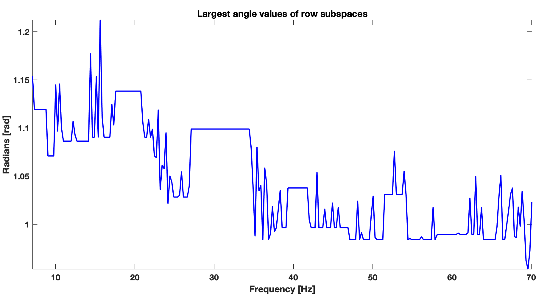
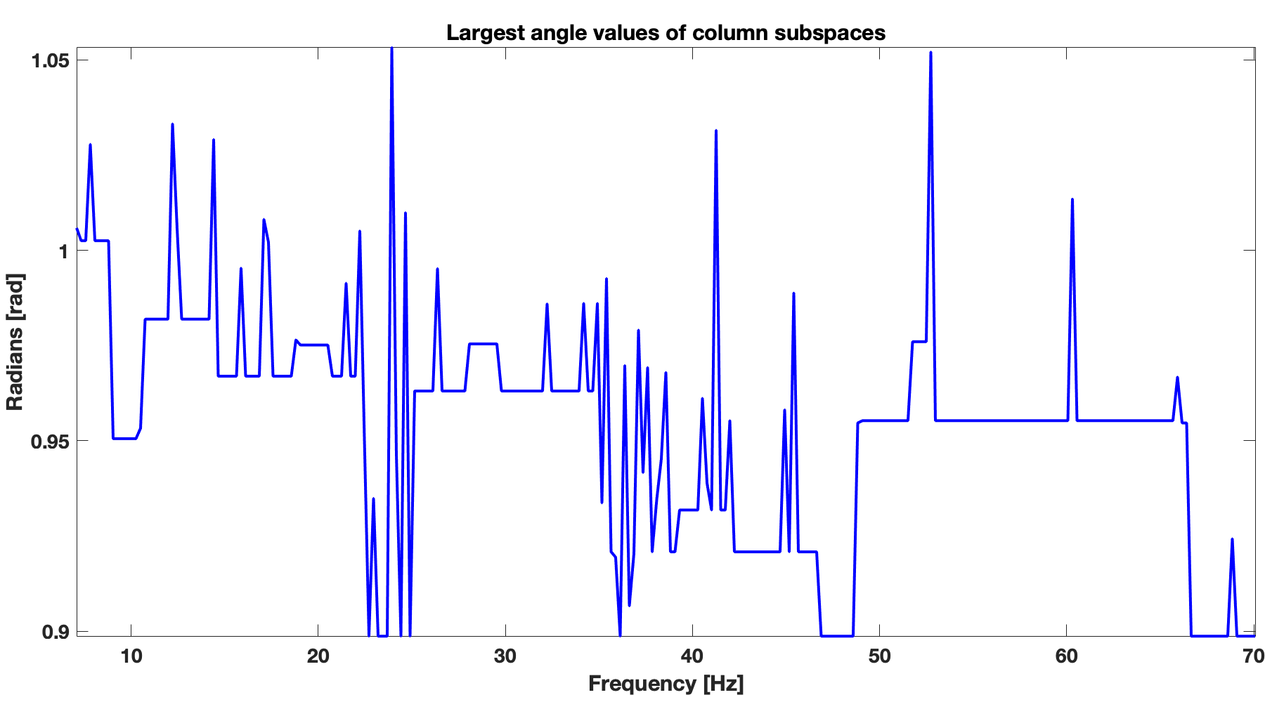
Figure 1 shows that as the frequency increase, the largest angles between the subspaces of neighboring frequencies decreases. Smaller the angle, more similar are subspaces. This angle test have demonstrated that the weighted matrix completion will perform better in high frequency band because of smaller angle in comparison to its lower frequency counterpart.

Numerical Experiments

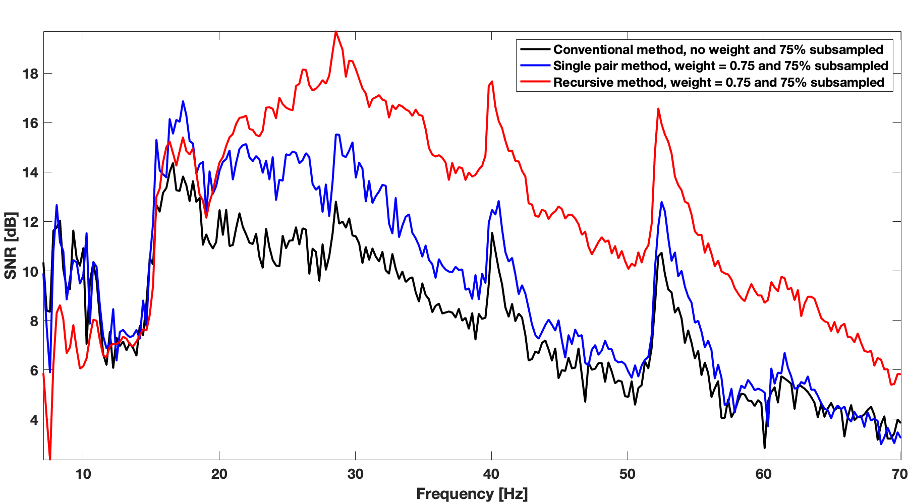
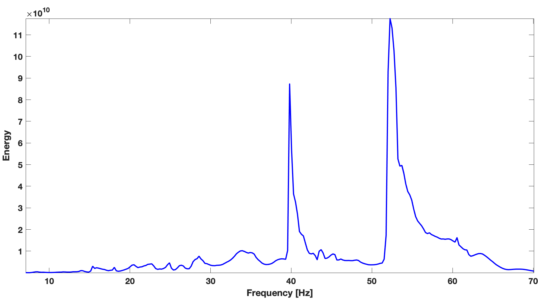
We demonstrate effectiveness of recursive weighted matrix completion method over the conventional matrix completion method and the weighted method just using previous frequency slice (named as single pair weighted method) in terms of data reconstruction quality. In single pair weighted method, we reconstruct previous frequency slice using conventional matrix completion. We use real \(2\)D seismic data with number of sources, \({ N }_{s}=354\), and number of receivers, \({ N }_{ r }=354\) acquired in Gulf of Suez for this comparison. Total number of time samples for this data set is \({ N }_{ t }=1024\) with sampling interval of \(0.004\, \mathrm{s}\). Most of the energy of the seismic line is concentrated in \(20\, \mathrm{Hz}\) to \(70\, \mathrm{Hz}\) frequency band (Figure 3b). To get the subsampled data (Figures 2b & 4b), we remove \(75 \%\) of sources using a jittered subsampling mask. Jittered subsampling method not only breaks the inherent properties such as low rank of fully sampled seismic data but also controls the maximum gap size of the incomplete data (Herrmann and Hennenfent, 2008). We show the results and comparisons in both frequency domain and time domain. For every frequency slice, we perform \(150\) iterations of spectral projected gradient algorithm for all these methods. Figure 2 shows results on a frequency slice at \(30\, \mathrm{Hz}\). Recovery with the unweighted method gives the result with S/R of \(11.43\, \mathrm{dB}\). Whereas recovery with the single pair weighted method gives a higher S/R of \(15.20\, \mathrm{dB}\), our recursive weighted method gives the highest S/R of of \(18.48\, \mathrm{dB}\), \(7.05\, \mathrm{dB}\) improvement in S/R over the unweighted method. Figure 2d, Figure 2f and Figure 2h show differences between these three different methods and ground truth data. The reconstruction using recursive prior knowledge gives the least residual in Figure 2h among these three methods. The residual of reconstruction without using any prior knowledge is Figure 2d and the residual of single pair weighted reconstruction is Figure 2f.

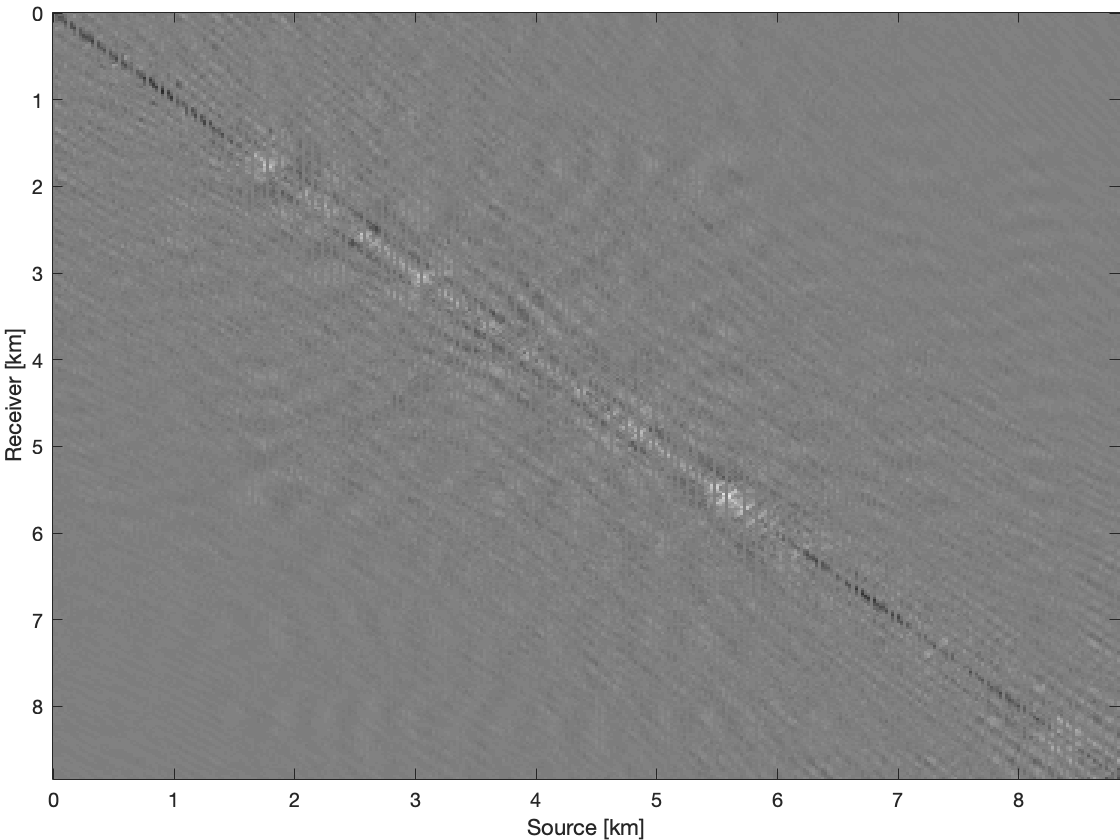
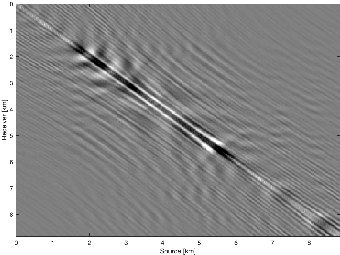
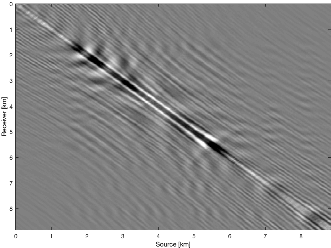
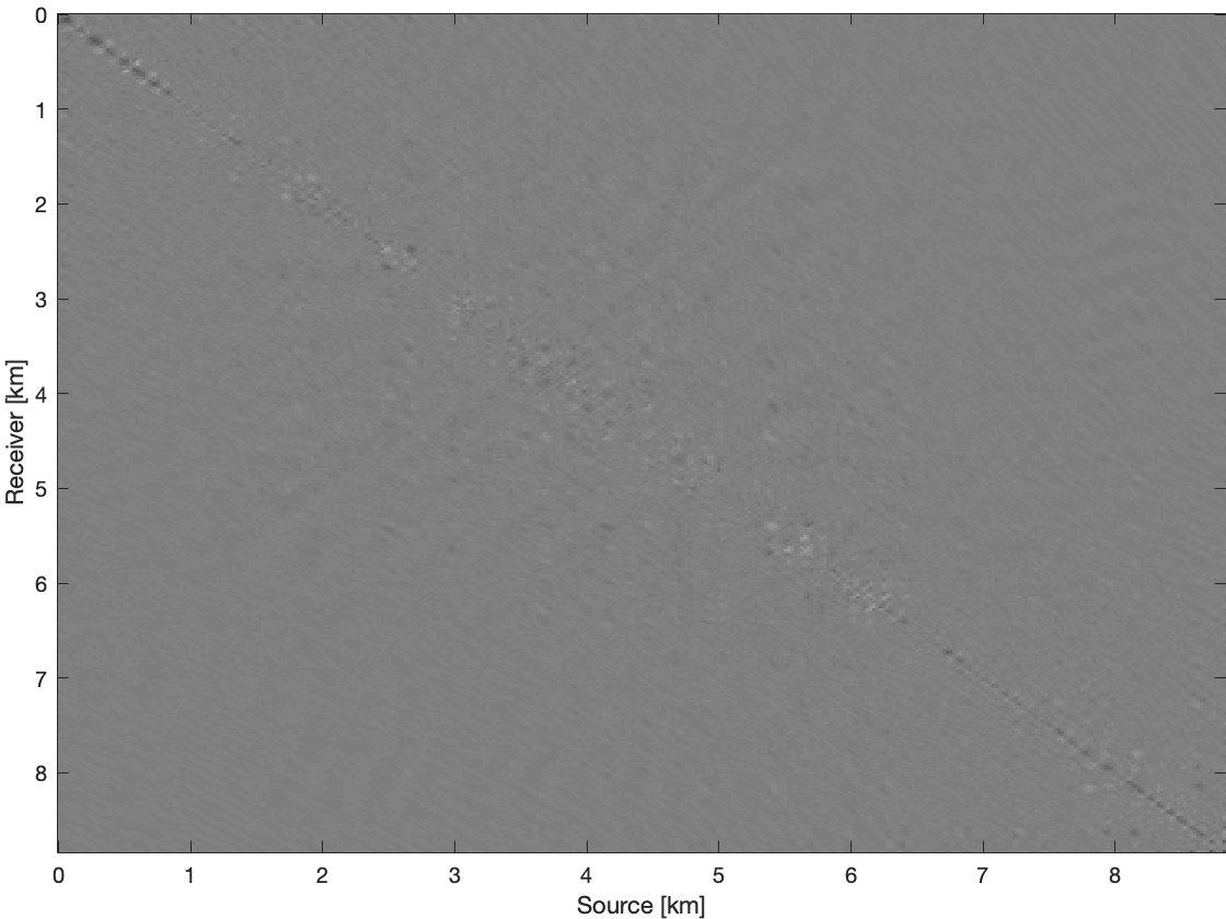
Figure 3a shows recursive weighted method’s performance (red color plot) over range of frequencies in terms of signal to noise of completion. Recursive weighted recovery clearly outperforms the conventional recovery without weight (black color plot in Figure 3a) and the single pair weighted recovery (blue color plot in Figure 3a) in the frequency range which contains most of the energy (Figure 3b).

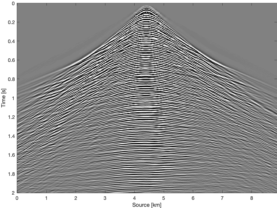
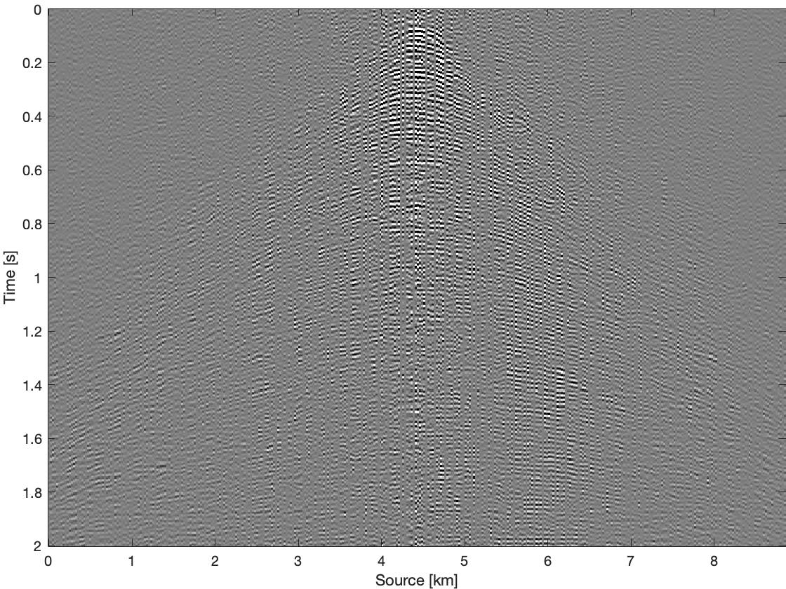
To further compare these three methods for time domain data, we apply them on all frequency slices and transfer results back to time domain. Figure 4 shows results and differences for one common receiver gather extracted from complete time domain data. With the conventional recovery we get S/R of \(6.87\, \mathrm{dB}\), whereas with single pair weighted recovery we get S/R of \(7.85\, \mathrm{dB}\) and with recursive weighted recovery we get S/R of \(11.63\, \mathrm{dB}\). With recursive weighted recovery we get almost \(5\, \mathrm{dB}\) improvement for complete time domain data over conventional recovery. It is also obvious to see the advantage of the recursive weighted method from three differences in Figure 4d, Figure 4f and Figure 4h. The residual is significantly reduced in Figure 4h in contrast to Figure 4d and Figure 4f.

Conclusions

In this work, we have proposed recursive weighted matrix completion to improve data reconstruction quality especially at high frequencies where the conventional matrix completion method performs poorly. In contrast to conventional low-rank matrix factorization without weighting or with non-recurrent pairwise weighting, our recursively weighted method performs better at the high frequencies, especially at frequencies where the data has the most energy. We also demonstrated the effectiveness of our recursive recovery on real data. Future work will be to extend the application of recursive weighted matrix completion to realistic size 3D seismic data reconstruction and also to simultaneous source acquisition.

Acknowledgement

The first and second authors have equal contribution to this work. This research was carried out as part of the SINBAD II project with the support of the member organizations of the SINBAD Consortium.