Large scale high-frequency wavefield reconstruction with recursively weighted matrix factorizations

Introduction

For economical extraction of hydrocarbon resources from the subsurface and to prevent hazardous situations oil and gas companies often rely on imaging and accurate estimates of the earth’s subsurface physical parameters such as wavespeed, density, etc. To obtain subsurface images and to recover these physical parameters, practitioners apply a series of processing steps to the raw seismic data collected from field during seismic data acquisition. Some of these processing steps, such as migration, demultiple, etc. require seismic data to be finely sampled and preferably on a regular grid. Unfortunately, seismic data acquisition on a fine regular grid is often prohibitively expensive and also operationally complex. Therefore, a general practice adapted by the oil and gas industry is to acquire seismic data on a coarse irregular grid, followed by wavefield reconstruction to a finer grid. In this work, we consider wavefield reconstruction from randomized samples taken from a periodic grid. The reader is referred to (Lopez et al., 2016) for an off-the-grid extension of presented wavefield reconstruction methodology.

In recent years, several methods for wavefield reconstruction have been developed. Many of these methods perform wavefield reconstruction in a transformed domain involving Fourier (S. Xu et al., 2005), Radon (Bardan, 1987), wavelet (Villasenor et al., 1996), or curvelet (F. J. Herrmann and Hennenfent, 2008) domain. To a varying degree, these transforms promote sparsity on seismic data, which is a key component of wavefield reconstruction based on compressive sensing (Candes et al., 2006; D. L. Donoho, 2006). While powerful, sparsity-based wavefield reconstruction does not scale well to 3D seismic where the data volumes become prohibitively large when structure is promoted along more than three dimensions, e.g. along all four source and receiver coordinates. By exploiting low-rank properties of matrices and tensors (Kumar et al., 2015; Oropeza and Sacchi, 2011), some of these high dimensional challenges have been overcome by building on early work of Recht et al. (2010), who extended some of the ideas of compressed sensing to matrices. Similar to CS, matrix completion relies on the fact that the underlying fully sampled data organized in a matrix permits a low-rank approximation. As in CS, randomized sampling breaks the low-rank structure, which informs (convex) optimization techniques that recover wavefields by minimizing the rank. Kumar et al. (2015) and Da Silva and Herrmann (2015) exploited this property and formalized matrix-/tensor-based wavefield reconstructions that are practical for large-scale seismic datasets (Kumar et al., 2017).

As demonstrated in the work by Kumar et al. (2015), low-rank matrix completion methods work well when reconstructing seismic data at the lower angular frequencies but the recovery quality degrades when we move to the higher frequencies (\(>15\, \mathrm{Hz}\)). This degradation in recovery quality is caused by the property that high-frequency frequency slices are not well approximated by low-rank matrix factorization (Kumar et al., 2015; A. Aravkin et al., 2014). Unfortunately, techniques such as multiple elimination and migration need access to high-frequency data to create high-fidelity artefact-free high-resolution images. This is especially true when physical properties are of interest in areas of complex geology.

To meet the challenges of recovering seismic data at high frequencies, we build on earlier work by A. Aravkin et al. (2014) and Eftekhari et al. (2018) who discussed how to improve the performance of low-rank matrix completion by including prior information in the form of weighting matrices. The weighting matrices are projections spanned by the row and column subspaces (and their complements) of a low-rank matrix factorization of a matrix that is close to the to-be-recovered matrix. As with weighted \(\ell_1\)-norm minimization, these weighting matrices improve the wavefield recovery if the principle angle between the subspaces of the weighting matrices and the to-be-recovered matrix is small. Conceptually, this is the matrix counterpart of weighted \(\ell_1\)-norm minimization proposed by Mansour et al. (2012). A. Aravkin et al. (2014) and Eftekhari et al. (2018) showed that wavefield recovery via matrix completion can be improved when low-rank factorizations from adjacent frequency slices are used to define these weighting matrices. A. Aravkin et al. (2014) used this principle assuming access to the low-rank factorization of an adjacent frequency slice using a modified version of the spectral-projected gradient algorithm (Van Den Berg and Friedlander, 2008). Also, Eftekhari et al. (2018) showed that for small principle angles, these weighing matrices reduce sampling requirement for successful data reconstruction by a logarithmic factor in comparison to the sampling requirement for the conventional matrix completion method.

While the initial results on wavefield reconstruction via weighted matrix completion were encouraging, the presented approach was not very practical because it relied on having access to the weights. In addition, the optimization relied on a computationally expensive optimization algorithm. We overcome these shortcomings by proposing a parallelizable recursive method that uses a recently developed alternating minimization procedure (Y. Xu and Yin, 2013; Jain et al., 2013) proposed by Lopez et al. (2015). Thanks to the recursive reconstruction, as first proposed by Y. Zhang et al. (2019), and the improved optimization we will demonstrate that we are able to improve the performance of our wavefield reconstruction algorithm.

The outline of our paper is as follows. We first provide a short overview of the principles of wavefield reconstruction via matrix completion. We follow this brief exposition by describing the challenges of high-frequency wavefield reconstruction and how these challenges can be addressed through weighted matrix completion. After this introduction, we describe how to derive a formulation in factored form, which allows to drastically reduce the problem size rendering our approach practical for 3D seismic data. In particular, we describe how our algorithm can be parallelized and applied to a large-scale high-frequency seismic wavefield reconstruction problem.

Wavefield reconstruction via weighted matrix completion

According to the seminal work of Recht et al. (2010), matrices that exhibit low-rank structure can be recovered from random missing entries through a nuclear norm minimization procedure. During the optimization the sum of the singular values is minimized. As long as the randomized subsampling decreases the rate of decay of the singular values, this type of minimization allows for the recovery of matrices that are well approximated by low-rank matrices when fully sampled. Kumar et al. (2015) used this principle to recover frequency slices from seismic lines in the midpoint-offset domain or from 3D seismic data permuted in non-canonical form (Da Silva and Herrmann, 2015). In either case, the resulting frequency slice can be approximated accurately by a low-rank matrix factorization.

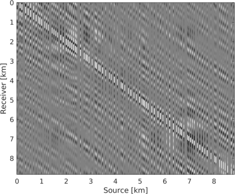
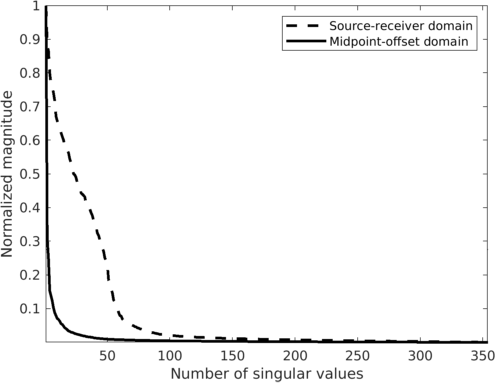
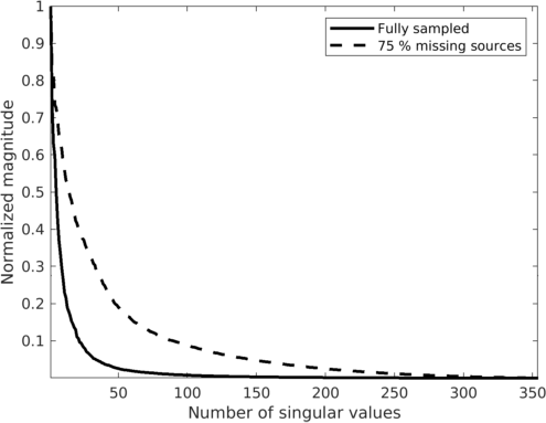
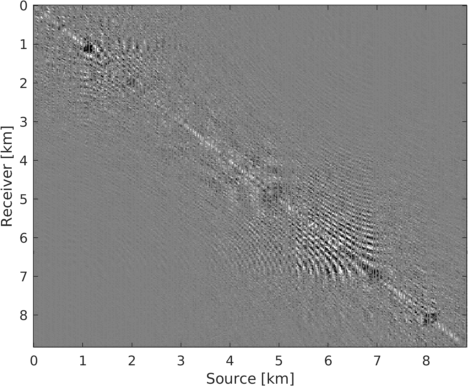
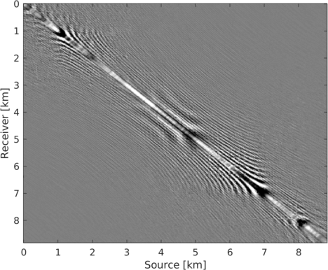
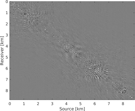
To illustrate the underlying principle of wavefield reconstruction via matrix completion, we consider a \(12\, \mathrm{Hz}\) monochromatic frequency slice assembled from a 2D line acquired in the Gulf of Suez. Figure 1, includes the real part of this frequency slice in the source-receiver and midpoint-offset domain after removing \(75\%\) of the sources via jittered subsampling (Hennenfent and Herrmann, 2008). Compared to uniform random subsampling, jittered subsampling controls the maximal spatial gap between sources, which favors wavefield reconstruction. While the monochromatic data contained in these frequency slices is comparable, the behavior of the singular values before and after subsampling is very different before and after transforming to the midpoint-offset domain (juxtapose Figures 2a and 2b). The singular values for the matricization in the shot-domain (denoted by the dashed lines) decay slowly when fully sampled and fast when subsampled, which can be understood since removing rows or columns from a matrix reduces the rank. The converse is true for data in the midpoint-offset domain, which shows a fast decay of the singular values for the fully sampled data and a slow decay after randomized subsampling. The latter creates favorable conditions for recovery via matrix completion (Kumar et al., 2015) via \[ \begin{equation} \vector{X} := \argmin_{\vector{Y}} \quad \|\vector{Y}\|_* \quad \text{subject to} \quad \|\mathcal{A}(\vector{Y}) - \vector{B}\|_{F} \leq \epsilon, \label{eqNucmin} \end{equation} \] which promotes low-rank matrices.

By solving this minimization problem, we aim to recover the minimum nuclear norm (\(\|\vector{X}\|_* = \sum\sigma_i\) with the sum running over the singular values of \(\vector{X}\)) of the complex-valued data matrix \(\vector{X} \in \mathbb{C}^{m \times n}\), with \(m\) offsets and \(n\) midpoints. Aside from minimizing the nuclear-norm objective, the minimizer fits the observed data \(\vector{B} \in \mathbb{C}^{m \times n}\) at the sampling locations to within some tolerance \(\epsilon\) measured by the Frobenious norm—i.e., \(\|\vector{D}\|_{F} = \sqrt{\sum_j \sum_k {D}_{jk}^2}\) for a matrix \(\vector{D}.\) In this expression, the linear operator \(\mathcal{A}\) implements the sampling mask putting zeros at source (and possibly receiver) locations that are not collected in the field. Here, the matrix \(\vector{Y}\) is the optimization variable. Equation \(\ref{eqNucmin}\) is similar to the classic Basis Pursuit DeNoising problem (BPDN, Van Den Berg and Friedlander, 2008) and can be solved with a modified version of the SPG\(\ell_1\) algorithm adapted for nuclear-norm minimization (A. Aravkin et al., 2014). To solve problem \(\ref{eqNucmin}\), SPG\(\ell_1\) solves a series of constrained subproblems during which the nuclear-norm constraint is relaxed to fit the observed data.

The challenge of high-frequency wavefield recovery

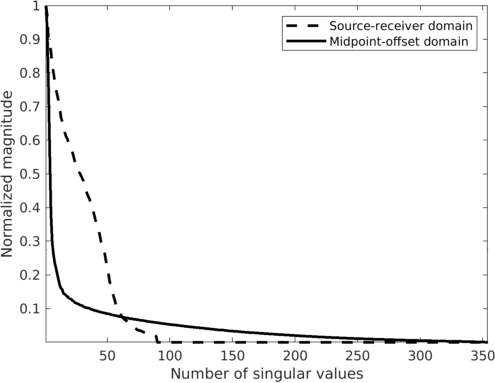
Wavefield reconstruction via matrix completion (cf. problem \(\ref{eqNucmin}\)) relies on the assumption that the singular values of monochromatic data organized in matrix decay rapidly. For the lower frequencies (\(< 15.0\, \mathrm{Hz}\)) this is indeed the case but unfortunately this assumption no longer holds for the higher frequencies. To illustrate this phenomenon, we compare in Figure 3 the decay of the singular values for the two matricizations of Figure 2 at \(12.0\, \mathrm{Hz}\) and \(60.0\, \mathrm{Hz}\). While the singular values at \(12.0\, \mathrm{Hz}\) indeed decay quickly this is clearly no longer the case at \(60.0\, \mathrm{Hz}\) (juxtapose solid lines in Figures 3a and 3b) where the singular values for the fully sampled data decay more slowly. This slower decay at the high frequencies is caused by the increased complexity and oscillatory behavior exhibited by data at higher temporal frequencies. Despite the fact that the randomized source subsampling slows the decay down, the slower decay of the fully sampled data leads to poor wavefield reconstruction (Figure 4a) and unacceptable large residuals (Figure 4b) at \(60.0\, \mathrm{Hz}\).

Weighted matrix completion

As Figures 3, 4a, and 4b illustrate, the success of wavefield reconstruction by minimizing the nuclear norm (cf. equation \(\ref{eqNucmin}\)) hinges on rapid decay of the singular values an assumption violated at the higher frequencies. This shortcoming can, at least in part, be overcome by using prior information from a related problem in the form of weights, an approach initially put forward by A. Aravkin et al. (2014) and further theoretically analyzed by Eftekhari et al. (2018). In its original form, the weights were derived from the reconstruction of the wavefield at a neighboring temporal frequency, which leads to a significant improvement for the reconstruction and the residual plotted in Figures 4c and 4d, respectively. By applying this approach recursively from low to high frequencies, Y. Zhang et al. (2019) improved the reconstruction even further judged by the quality of Figure 4e and the size of the residual plotted in Figure 4f. In this work, we further extend this result by reformulating the optimization problem and by introducing a parallel algorithm that limits communication.

We obtained the above weighted wavefield reconstructions by minimizing (A. Aravkin et al., 2014; Eftekhari et al., 2018) \[ \begin{equation} \vector{X} := \argmin_{\vector{Y}} \quad \|\vector{Q}\vector{Y}\vector{W}\|_* \quad \text{subject to} \quad \|\mathcal{A}(\vector{Y}) - \vector{B}\|_F \leq \epsilon, \label{eqWeighted} \end{equation} \] where the weighting matrices \(\vector{Q} \in \mathbb{C}^{m \times m}\) and \(\vector{W} \in \mathbb{C}^{n \times n}\) are projections given by \[ \begin{equation} \vector{Q} = {w}_{1}\vector{U}\vector{U}^H + \vector{U}^\perp \vector{U}^{{\perp}^{H}} \label{eqQ} \end{equation} \] and \[ \begin{equation} \vector{W} = {w}_{2}\vector{V}\vector{V}^H + \vector{V}^\perp \vector{V}^{{\perp}^{H}}, \label{eqV} \end{equation} \] where the symbol \(^H\) denotes complex transpose. These projections are spanned by the row and column subspaces \(\vector{U}\), \(\vector{V}\) and their orthogonal complements \(\vector{U}^\perp\) and \(\vector{V}^\perp\). Also, these subspaces \(\vector{U}\), \(\vector{V}\) have orthonormal columns making \(\vector{U}\vector{U}^H\) and \(\vector{V}\vector{V}^H\) orthogonal projections. The pair of matrices \(\{\mathbf{U},\mathbf{V}\}\) are low rank and can be obtained from the factorization of a lower adjacent frequency slice. The choice for the weights \({w}_1\) and \({w}_2\) in equations \(\ref{eqQ}\) and \(\ref{eqV}\) depends on the similarity between the corresponding row and column subspaces of the two adjacent frequency slices. We follow Eftekhari et al. (2018) and quantify this similarity by the largest principle angle between these subspaces. The smaller this angle, the more similar the subspaces from the two adjacent frequency slices will be. In situations where the adjacent frequency slices are near orthogonal—i.e., have a near \(90^\circ\) angle, we choose \({w}_{1}\uparrow 1\) and \({w}_{2} \uparrow 1\) so that the weighting matrices \(\vector{Q}\) and \(\vector{W}\) become identity matrices. In that case, the weighting matrices should not add information—i.e., the solution of problem \(\ref{eqWeighted}\) should become equivalent to solving the original problem in equation \(\ref{eqNucmin}\). Conversely, when the subspaces are similar—i.e., they have an angle \(\ll 90^\circ\), then the \({w}_{1}\) and \({w}_{2}\) should be chosen small such that we penalize solutions more in the orthogonal complement space. Depending on our confidence in the given factorization, we chose these weights close to one when we have little confidence and close to zero when we have more confidence.

While replacing the nuclear-norm objective in equation \(\ref{eqNucmin}\) by its weighted counterpart in equation \(\ref{eqWeighted}\) is a valid approach responsible for improvements reported in Figure 4, its solution involves non-trivial weighted projections (see equation \(7.3\) in A. Aravkin et al., 2014). These computationally costly operations can be avoided by rewriting optimization problem \(\ref{eqWeighted}\) in a slightly different form where the weights are moved from the objective to the data constraint—i.e., we have \[ \begin{equation} \vector{\bar X} := \argmin_{\vector{\bar Y}} \quad \|\vector{\bar Y}\|_* \quad \text{subject to} \quad \|\mathcal{A}(\vector{Q}^{-1}\vector{\bar Y}\vector{W}^{-1}) - \vector{B}\|_F \leq \epsilon. \label{eqWeightednew} \end{equation} \] In this formulation, the optimization is carried out over the new variable \(\vector{\bar Y} = \vector{Q}\vector{Y}\vector{W}\). After solving for this variable, we recover the solution of the original problem \(\vector{X}\) from \(\vector{\bar X}\) as follows: \(\vector{X} = \vector{Q}^{-1}\vector{\bar X}\vector{W}^{-1}\). We arrived at this formulation by using the fact that the matrices \(\vector{Q}\) and \(\vector{W}\) are invertible (for non-zeros weights \({w}_{1}\) and \({w}_{2}\)) with inverses given by \[ \begin{equation} \vector{Q}^{-1} = \frac{1}{w}_{1}\vector{U}\vector{U}^H + \vector{U}^\perp \vector{U}^{{\perp}^{H}} \label{eqQinv} \end{equation} \] and \[ \begin{equation} \vector{W}^{-1} = \frac{1}{w}_{2}\vector{V}\vector{V}^H + \vector{V}^\perp \vector{V}^{{\perp}^{H}}. \label{eqWinv} \end{equation} \] Because we moved the weighting matrices to the data constraint, we no longer have to project onto a more complicated constraint as in A. Aravkin et al. (2014), which results in solutions of equation \(\ref{eqWeightednew}\) at almost the same computational costs as in the original formulation (Equation \(\ref{eqNucmin}\)). This formulation forms the basis for our approach to wavefield reconstruction that is capable of handling the large data volumes of 3D seismic.

Scalable multi-frequency seismic wavefield reconstruction

So far, our minimization problems relied on explicit formation of the data matrix and on the singular-value decomposition (SVD, A. Aravkin et al. (2014)) both of which are unfeasible for industry-scale 3D wavefield reconstruction problems. To address this issue, we discuss how to recast the above weighted matrix completion approach into factored form, which has computational benefits and, as we will show below, can still be parallelized.

Weighted low-rank matrix factorization

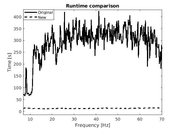
To avoid computing costly SVDs, we first cast the solution of equation \(\ref{eqWeightednew}\) into factored form: \[ \begin{equation} \begin{split} \vector{\bar L}, \vector{\bar R} := \argmin_{\vector{\bar L_\#}, \vector{\bar R_\#}} \quad \frac{1}{2} {\left\| \begin{bmatrix} \vector{\bar L_\#} \\ \vector{\bar R_\#} \end{bmatrix} \right\|}_F^2 \quad \text{subject to} \quad \|\mathcal{A}(\vector{Q}^{-1}\vector{\bar L_\#}\vector{\bar R_\#}^{H}{\vector{W}^{-H}}) - \vector{B}\|_{F} \leq \epsilon, \end{split} \label{eqWeighteLRopt} \end{equation} \] where \(\vector{\bar L} = \vector{Q}\vector{L}\) and \(\vector{\bar R} = \vector{W}\vector{R}\). Under certain technical conditions (Candes and Recht, 2009), which include choosing the proper rank \(r\), the factored solution, \(\vector{X}=\vector{L}\vector{R}^H\) with \(\vector{L} = \vector{Q}^{-1}\vector{\bar L}\) and \(\vector{R} = \vector{W}^{-1}\vector{\bar R}\), corresponds to the solution of the weighted problem included in equation \(\ref{eqWeighted}\). Here, the matrices \(\vector{L} \in \mathbb{C}^{m \times r}\) and \(\vector{R} \in \mathbb{C}^{n \times r}\) are the low-rank factors of \(\vector{X}\). Using the property that the matrices \(\vector{W}^{H} = \vector{W}\) and \(\vector{Q}^{H} = \vector{Q}\) in equation \(\ref{eqWeighteLRopt}\) are idempotent, we replace \(\vector{W}^{-H}\) by \(\vector{W}^{-1}\) to avoid extra computation. Compared to the original convex formulation, equation \(\ref{eqWeighteLRopt}\) can be solved with alternating optimization, which is computationally efficient as evidenced from the runtimes plotted in Figure 5 as a function of temporal frequency. Of course, this approach only holds as long as the monochromatic data matrices can be well approximated by low rank matrices—i.e., \(r\ll\min(m,n)\).

While the above weighted formulation allows us to solve the problem in factored form, it needs access to the subspaces \(\{\mathbf{U},\mathbf{V}\}\), which requires computing the full SVD (Eftekhari et al., 2018). Since we cannot compute this full SVD, we instead orthogonalize the low-rank factors from adjacent frequency slices themselves by carrying out computationally cheap SVDs on the factors rather than on the full data matrix and then keeping the top \(r\) left singular vectors. This approach is justified because orthogonalizing low-rank factors allows approximating orthogonal subspaces spanned by the full frequency slice.

The results presented in Figure 4 were obtained in factored form and demonstrated clearly how the incorporation of weight matrices improves recovery especially when these weight matrices are calculated recursively from low to high frequencies (juxtapose Figures 4c, 4d and 4e, 4f). This improvement is due to the fact that low-frequency data matrices can be better approximated by low-rank matrices, which improves the recovery and therefore the weighted reconstruction.

Weighted parallel recovery

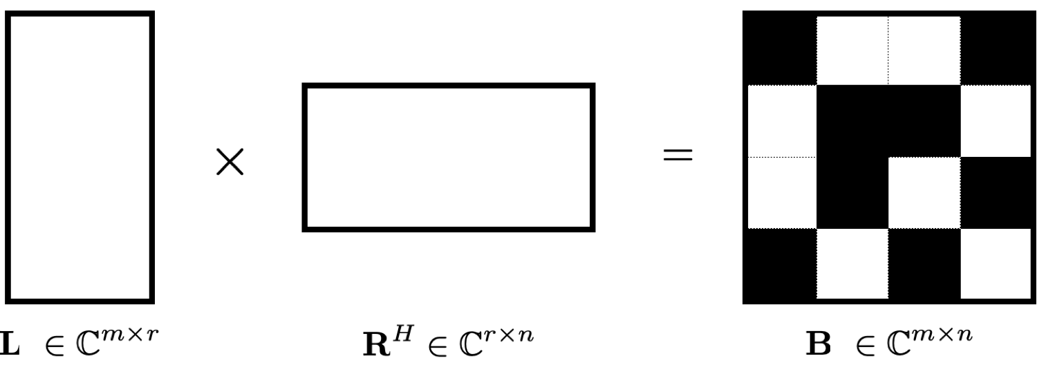
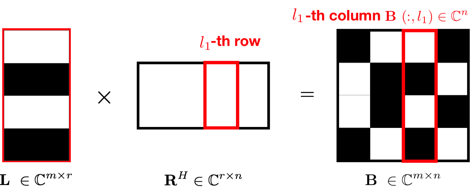
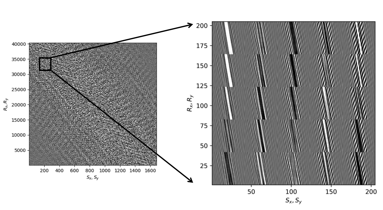
The example in Figure 4 made it clear that wavefield reconstruction via matrix factorization improves when including weight matrices that carry information on the row and column subspaces. However, inclusion of these weight matrices makes it more difficult to parallelize the algorithm because the parallelized alternating optimization approach by Recht and Ré (2013) and Lopez et al. (2015) no longer applies straightforwardly. That approach relies on decoupled computations on a row-by-row and column-by-column basis (see Figure 6) in which case one alternates between minimizing the rows via \[ \begin{equation} \vector{R}(l_1,:)^{H} := \argmin_{\vector{v}} \quad \frac{1}{2} {\left\| \vector{v} \right\|}^2 \quad \text{subject to} \quad \|\mathcal{A}_{l_1}(\vector{L}\vector{v}) - \vector{B}(:,l_1)\| \leq \gamma \label{eqpalunweightedL} \end{equation} \] for \(l_1 = 1\cdots n\) and the columns via \[ \begin{equation} \vector{L}(l_2,:)^{H} := \argmin_{\vector{u}} \quad \frac{1}{2} {\left\| \vector{u} \right\|}^2 \quad \text{subject to} \quad \|\mathcal{A}_{l_2}((\vector{R}\vector{u})^{H}) - \vector{B}(l_2,:)\| \leq \gamma \label{eqpalunweightedR} \end{equation} \] for \(l_2 = 1\cdots m\). With this approach, the rows of the right factor \(\mathbf{R}\) are updated first by iterating over the rows via the index \(l_1=1\cdots n\). These updates are followed by updates on the rows of the left \(\mathbf{L}\) factor by iterating over the rows via the index \(l_2=1\cdots m\). Contrary to the serial problem, these optimizations are conducted on individual vectors \(\vector{v} \in \mathbb{C}^{r}\) and \(\vector{u} \in \mathbb{C}^{r}\) in parallel because they decouple—i.e., the \(l_1,l_2\)th row of \(\vector{R}, \vector{L}\) only involve the \(l_1, l_2\)th column/row of the observed data matrix \(\vector{B}\) and submatrices \(\mathcal{A}_{l_1}, \mathcal{A}_{l_2}\) that act on these columns/rows. To simplify notation, we introduced the symbol \(:\) to extract the \(l_1\)th column, \(\vector{B}(:,l_1)\), or \(l_2\)th row, \(\vector{B}(l_2,:)\). As before, we allow for the presence of noise by solving the optimizations to within a user-specified \(\ell_2\)-norm tolerance \(\gamma\).

Because the operations in equations \(\ref{eqpalunweightedL}\) and \(\ref{eqpalunweightedR}\) decouple, they allow for a parallel implementation that scales well for large-scale industrial 3D seismic problems. However, the decoupled formulation does not include weighting matrices limiting its usefulness for recovery problems at higher frequencies that require weighting matrices. Below we present a novel approach to ameliorate this problem in which we take equations \(\ref{eqpalunweightedL}\) and \(\ref{eqpalunweightedR}\) as a starting point and pre- and post multiply the data misfit terms by \(\mathbf{Q}\) and \(\mathbf{W}\) after including the weighting matrices as in equation \(\ref{eqWeighteLRopt}\). Next, we use the property that for large weights, the matrices \(\mathbf{Q}\) and \(\mathbf{W}\) nearly commute with the measurement operator \(\mathcal{A}\)—i.e., we have \(\mathbf{Q}\mathcal{A}(\mathbf{Q}^{-1}\mathbf{\bar{X}W}^{-1})\approx\mathcal{A}(\mathbf{\bar{X}W}^{-1})\) and \(\mathcal{A}(\vector{Q}^{-1}\mathbf{\bar{X}W}^{-1})\vector{W}\approx \mathcal{A}(\vector{Q}^{-1}\mathbf{\bar{X}})\) where \(\mathbf{\bar{X}}\) represents the fully sampled data matrix or its factored form. With these approximations, we arrive at the following weighted iterations: \[ \begin{equation} \vector{\bar R}(l_1,:)^{H} := \argmin_{\vector{\bar v}} \quad \frac{1}{2} \left\|\vector{\bar v}\right\|_2^2 \quad \text{subject to} \quad \|\mathcal{A}_{l_1}(\vector{Q}^{-1}\vector{\bar L}\vector{\bar v}) - \vector{B}_R(:,l_1)\| \leq \gamma \label{eqwtRpar} \end{equation} \] for \(l_1 = 1\cdots n\) and \[ \begin{equation} \vector{\bar L}(l_2,:)^{H} := \argmin_{\vector{\bar u}} \quad \frac{1}{2} \left\|\vector{\bar u}\right\|^2 \quad \text{subject to} \quad \|\mathcal{A}_{l_2}((\vector{\bar R}\vector{\bar u})^{H}\vector{W}^{-1}) - \vector{B}_L(l_2,:)\| \leq \gamma \label{eqwtLpar} \end{equation} \] for \(l_2 = 1\cdots m\). In these expressions, we replaced the incomplete data matrix by \(\mathbf{B}_R=\mathbf{B}\mathbf{W}\) and \(\mathbf{B}_L=\mathbf{Q}\mathbf{B}\), respectively. This means that we pre- and post-multiply the observed monochromatic data matrix \(\mathbf{B}\) with \(\mathbf{Q}\) and \(\mathbf{W}\) before extracting its columns or rows.

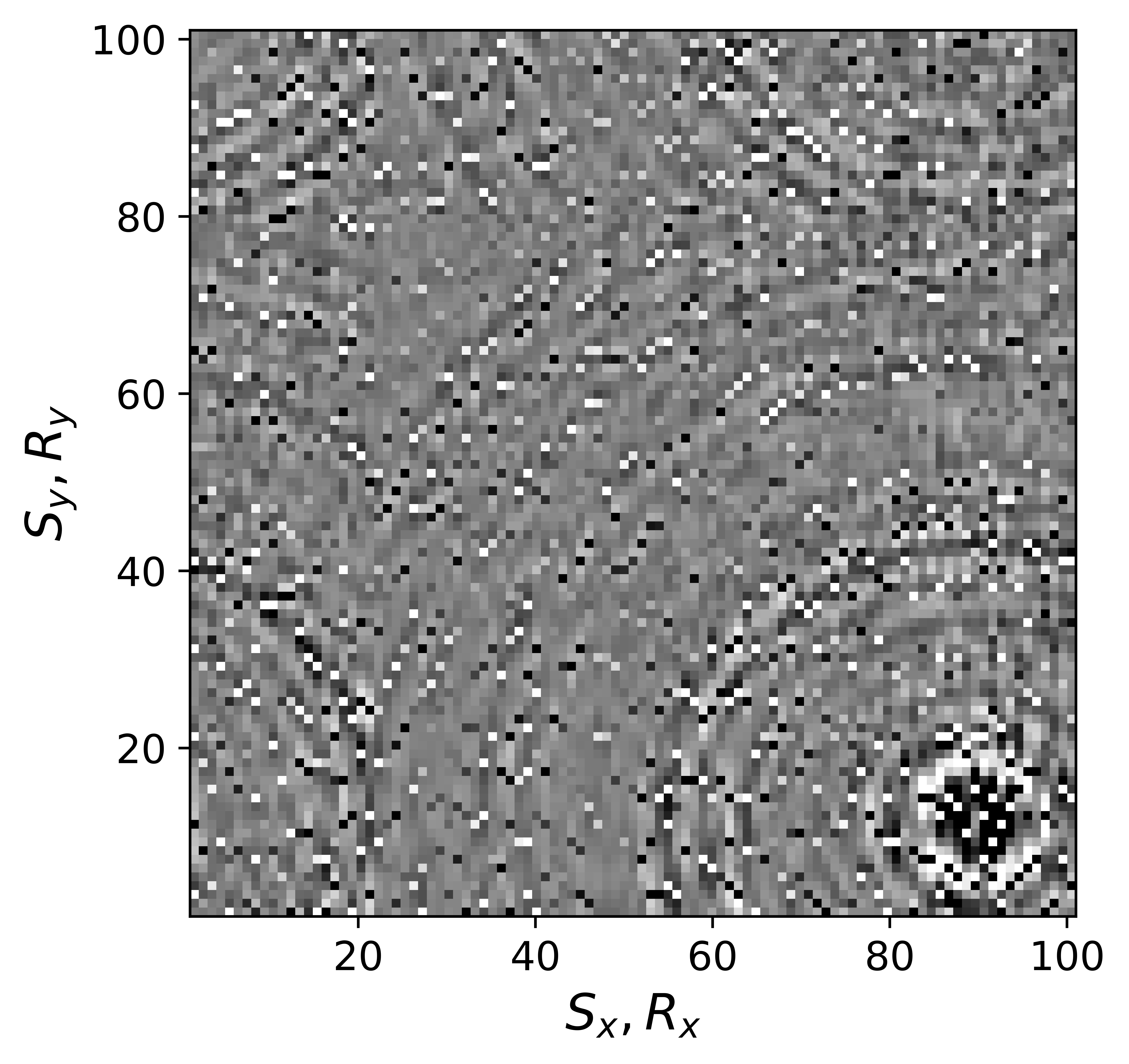
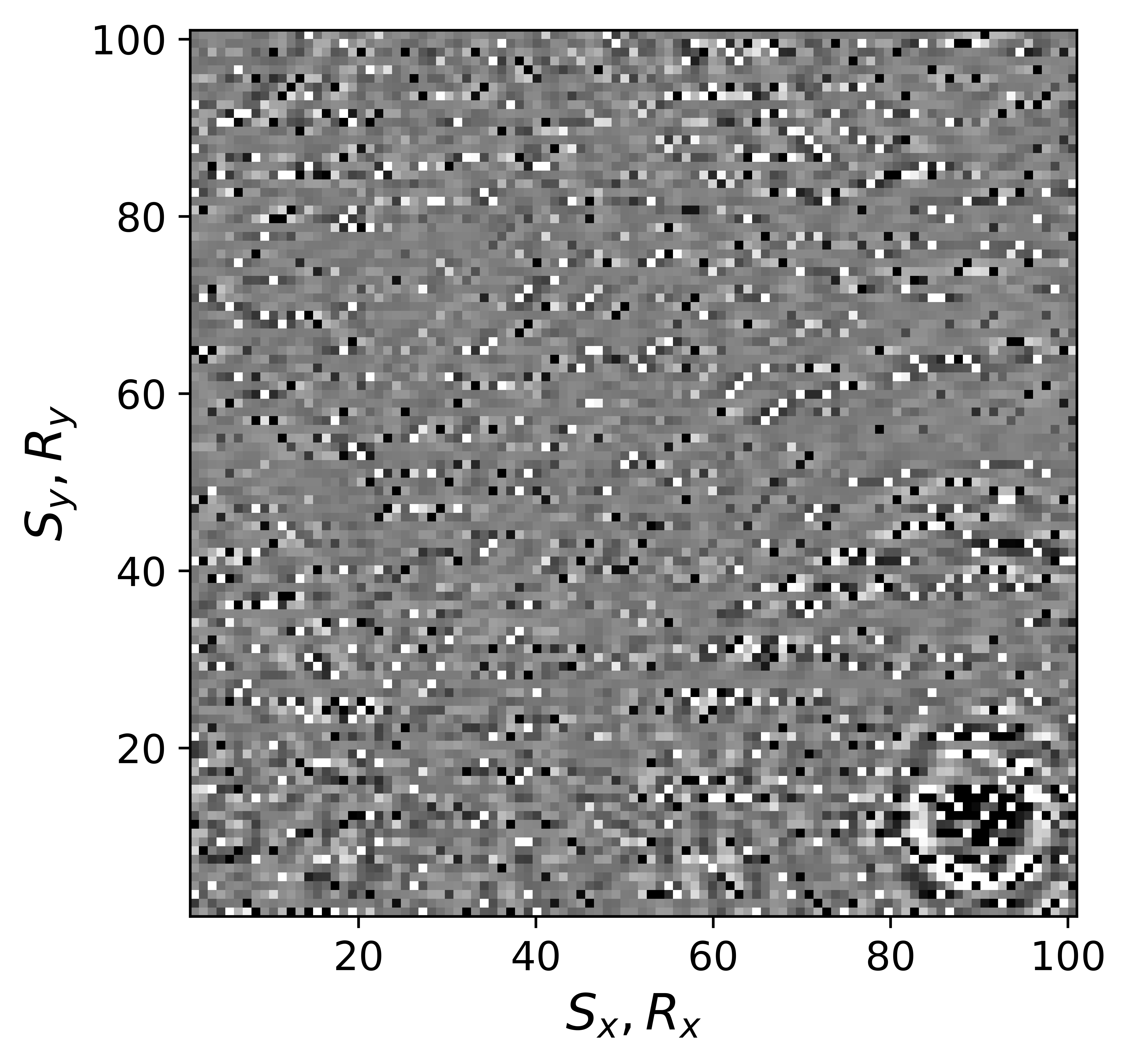
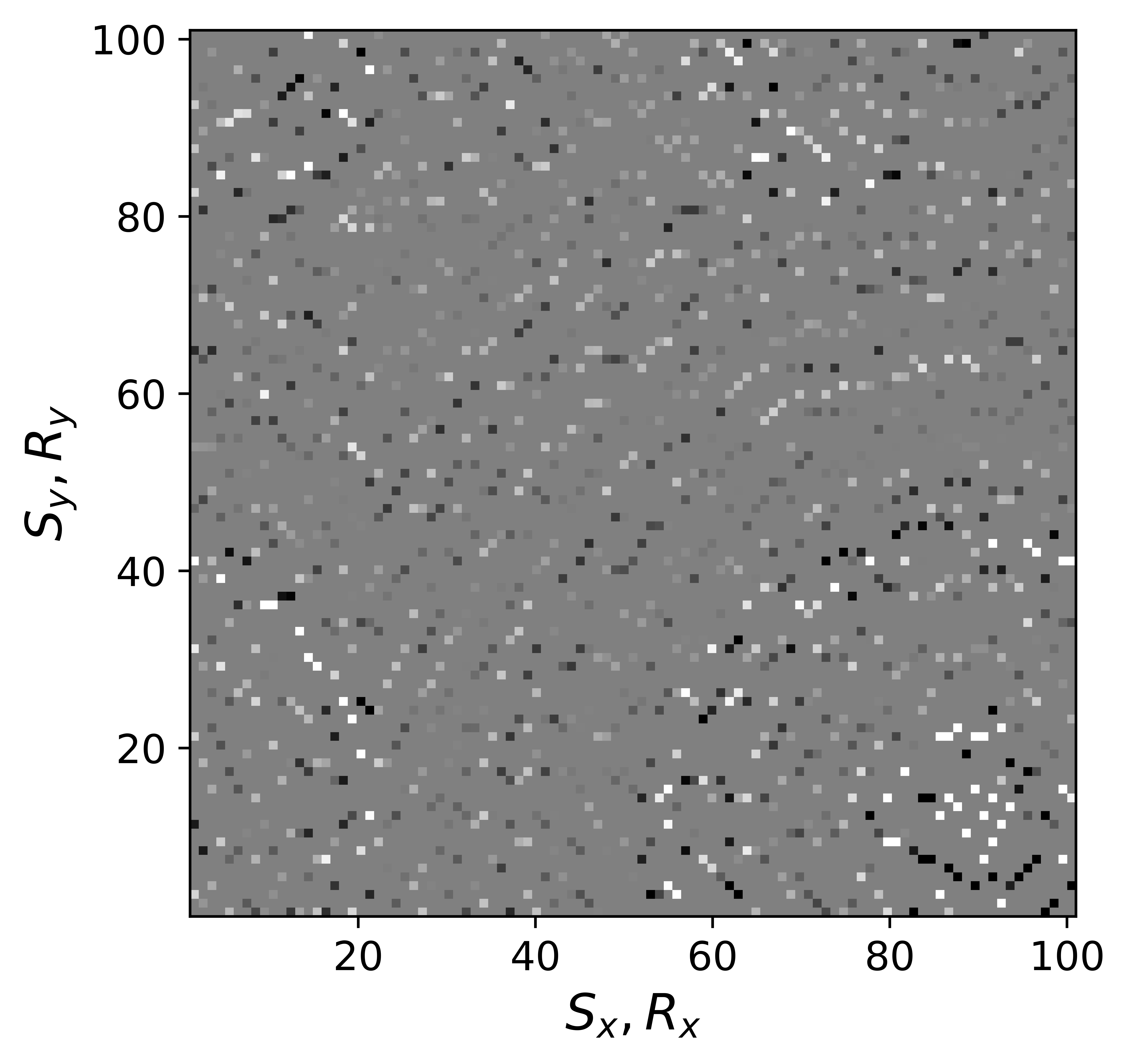
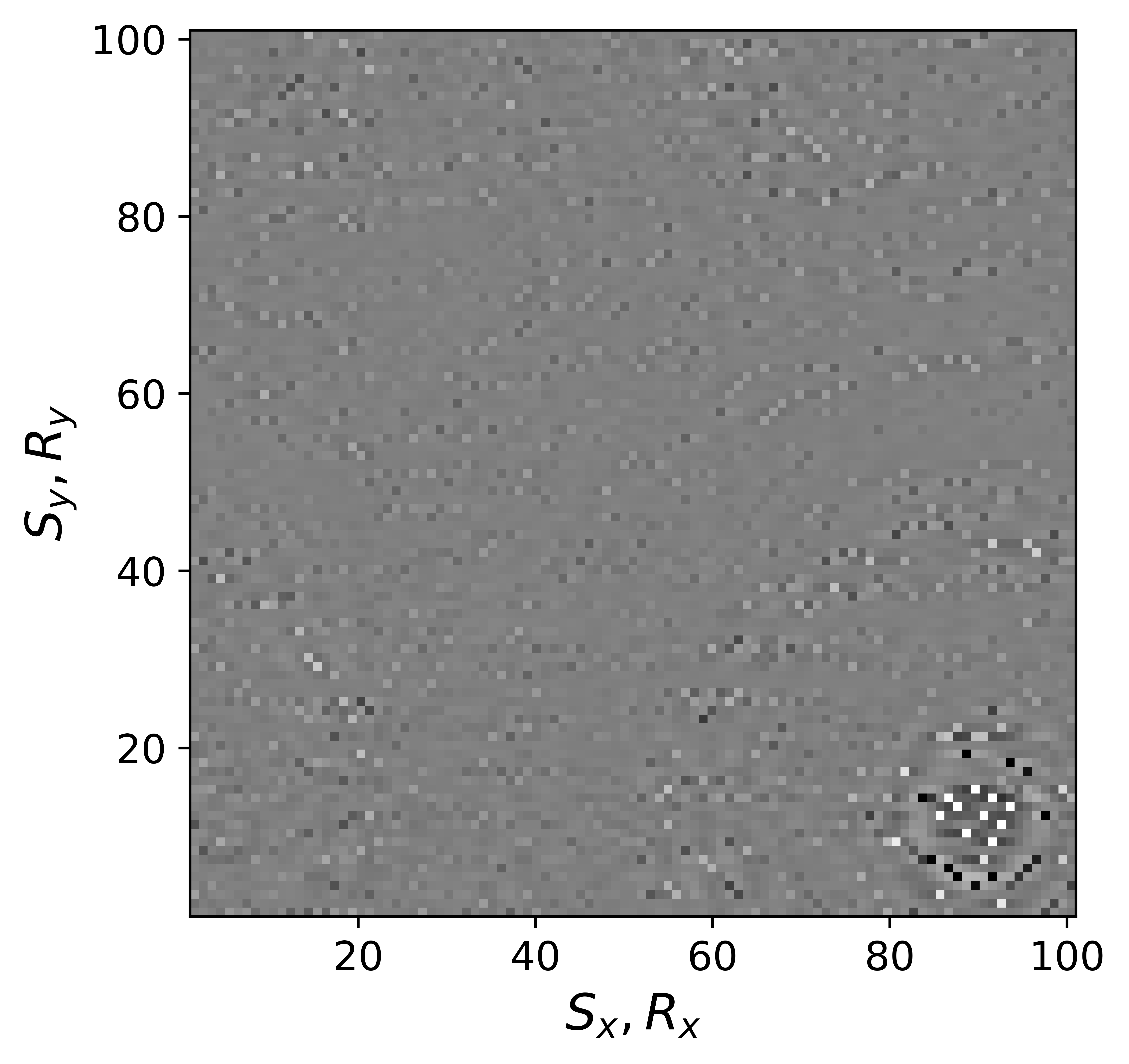
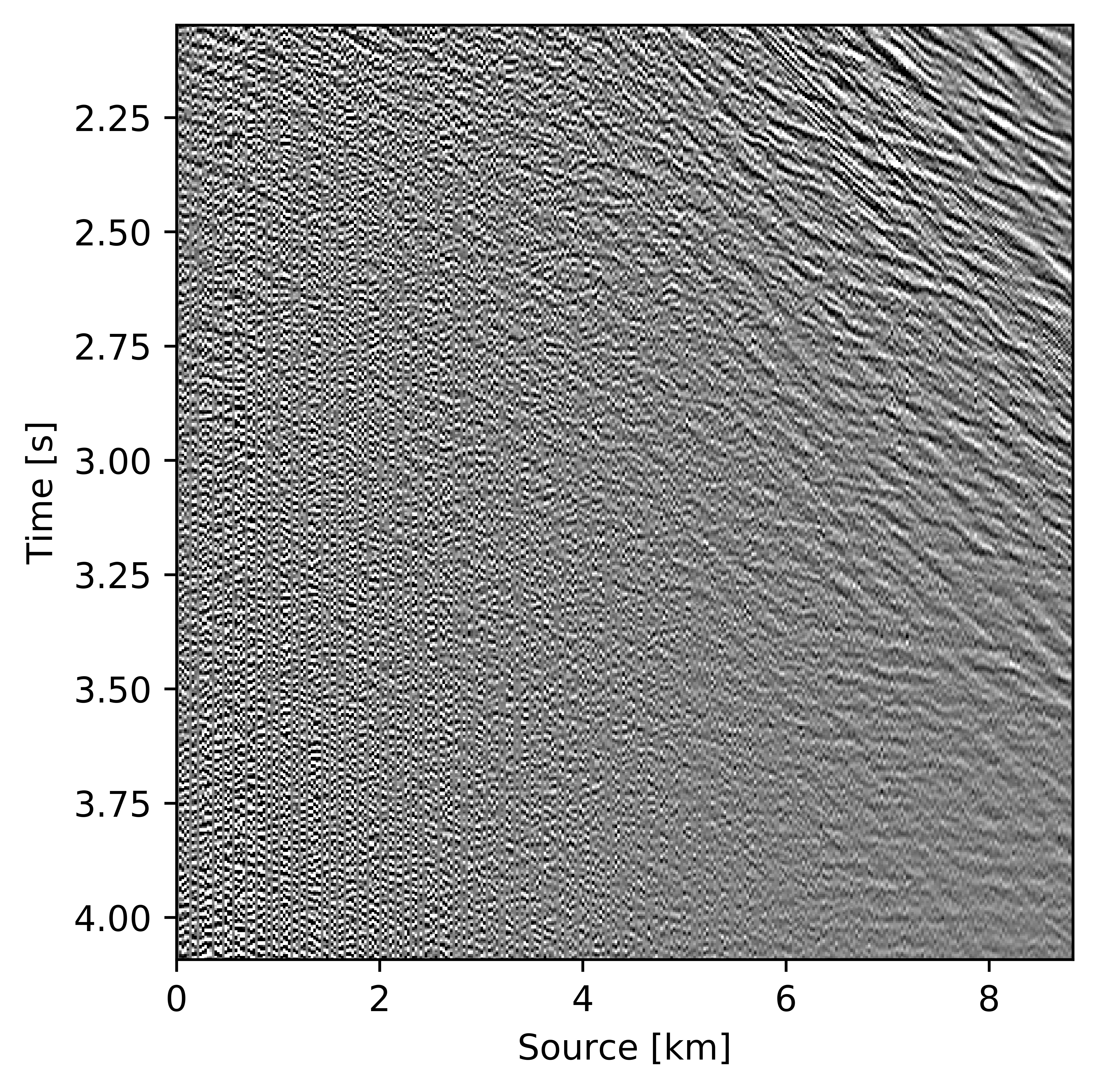
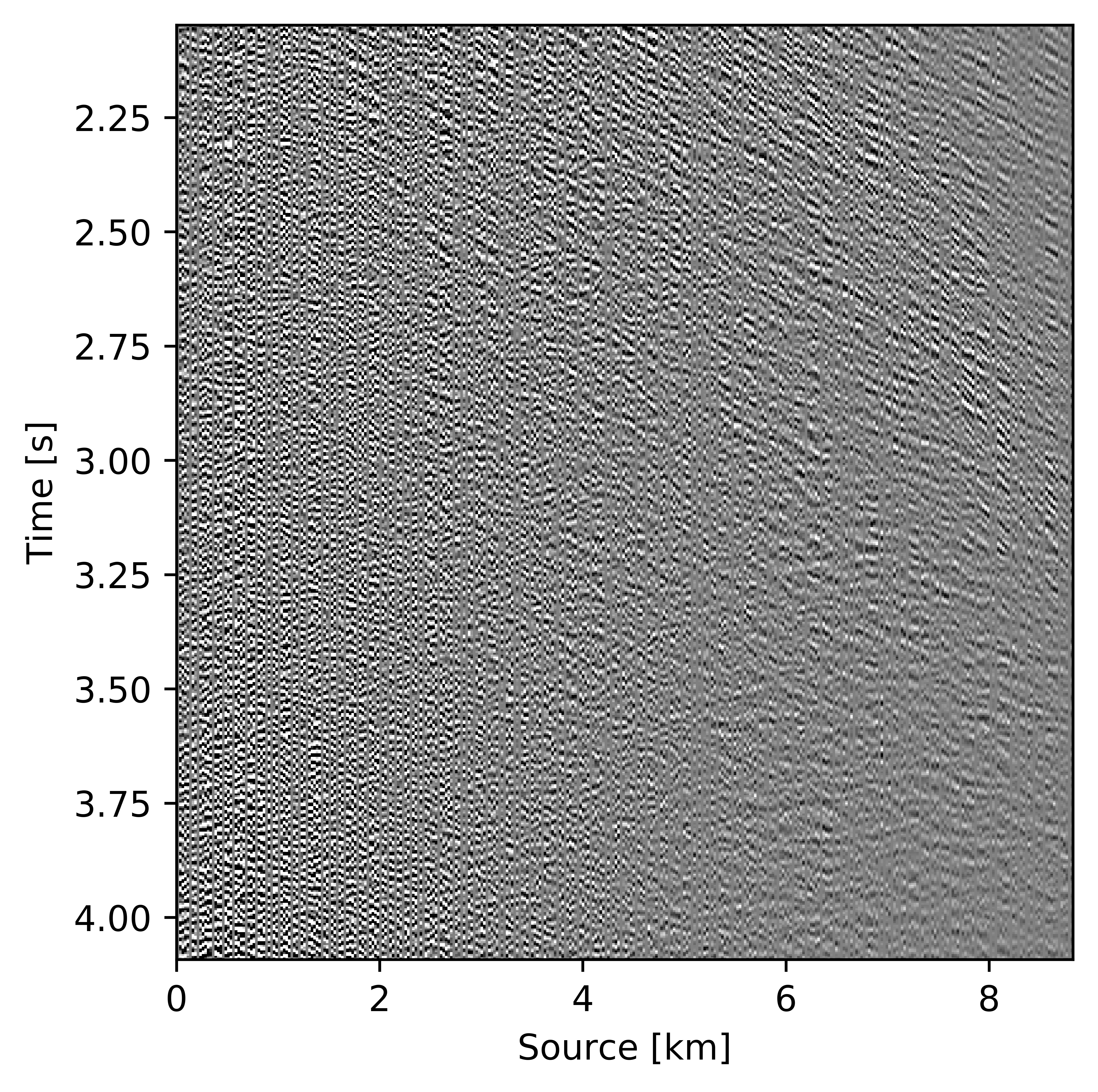
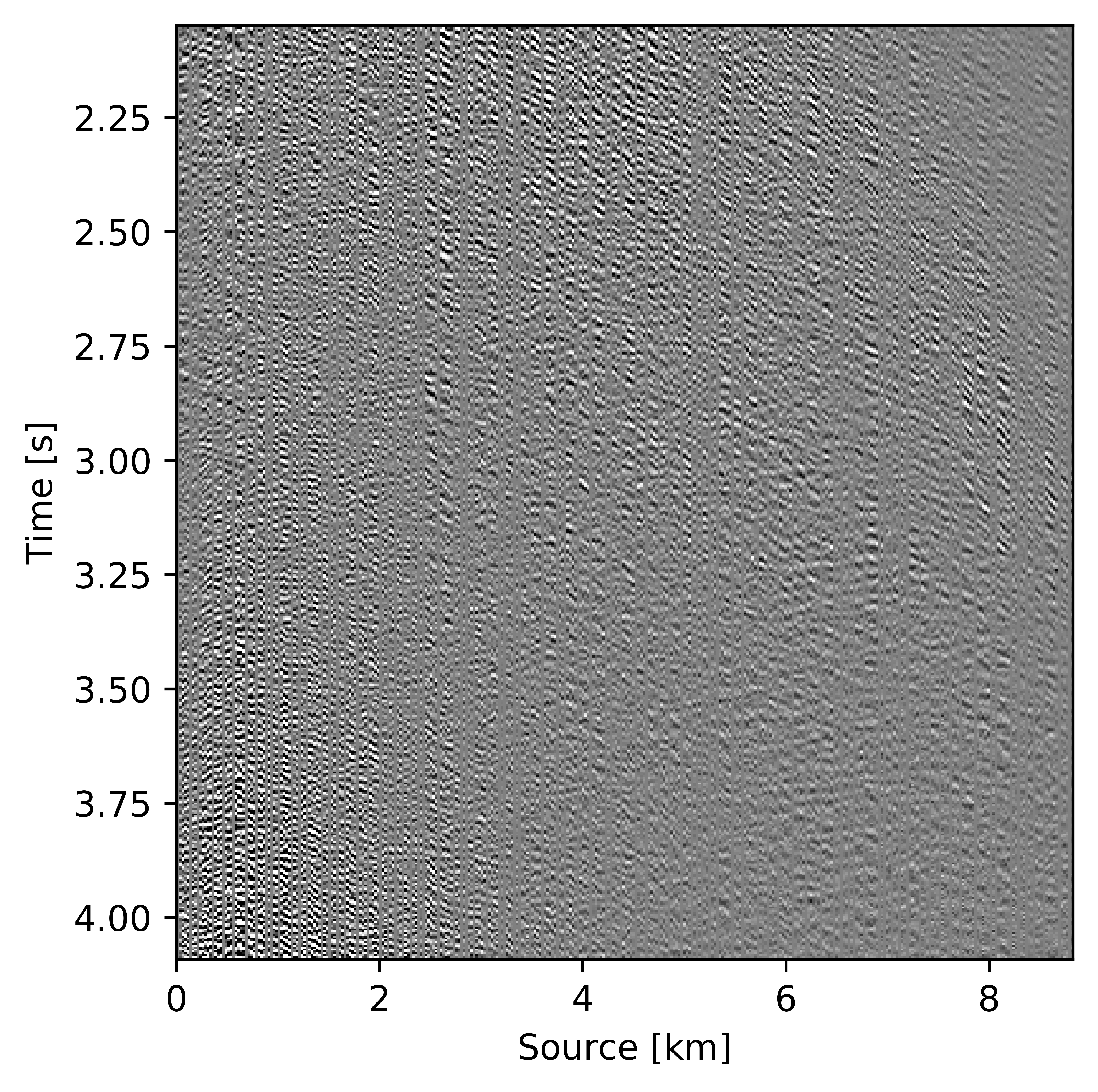
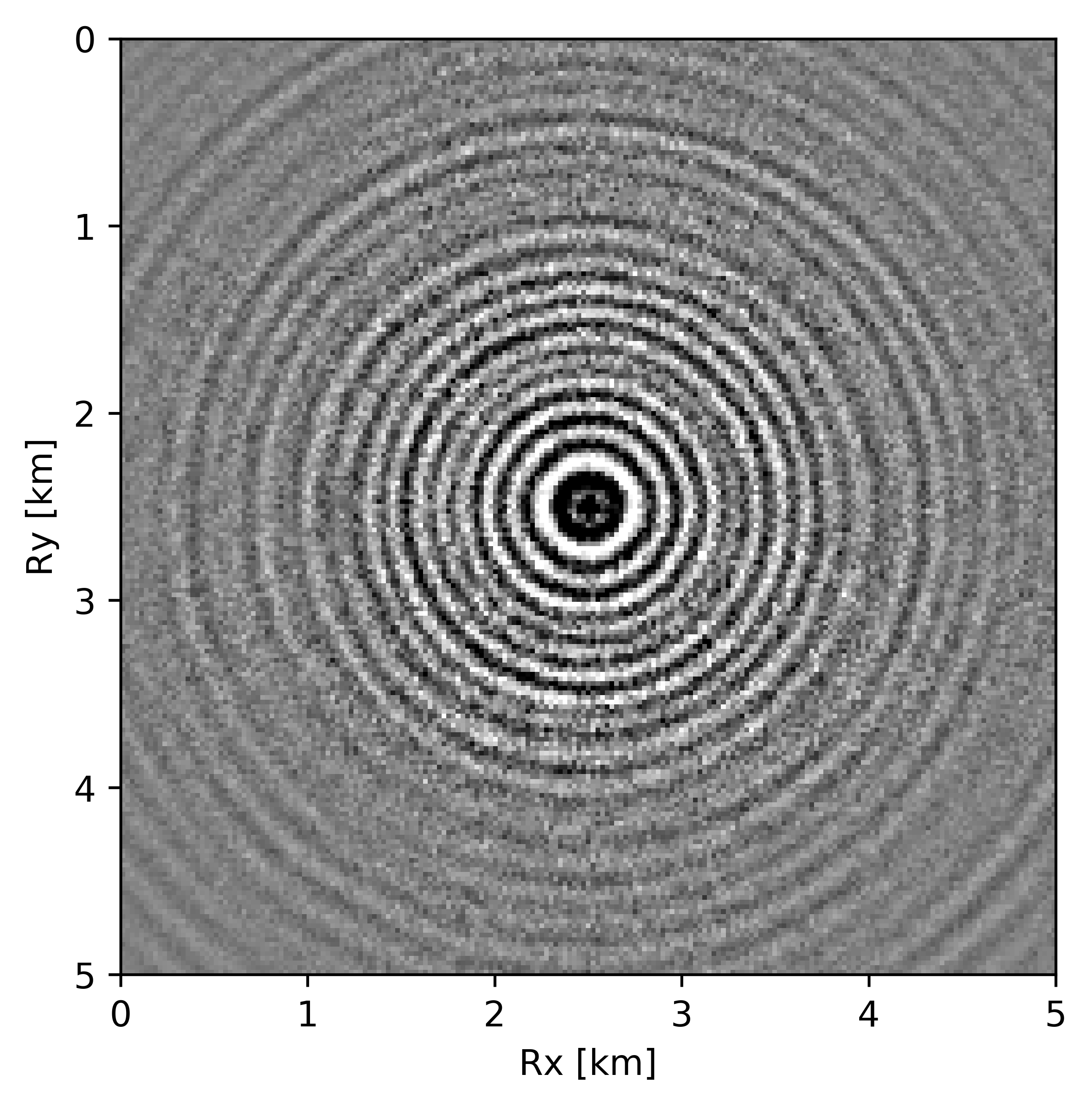
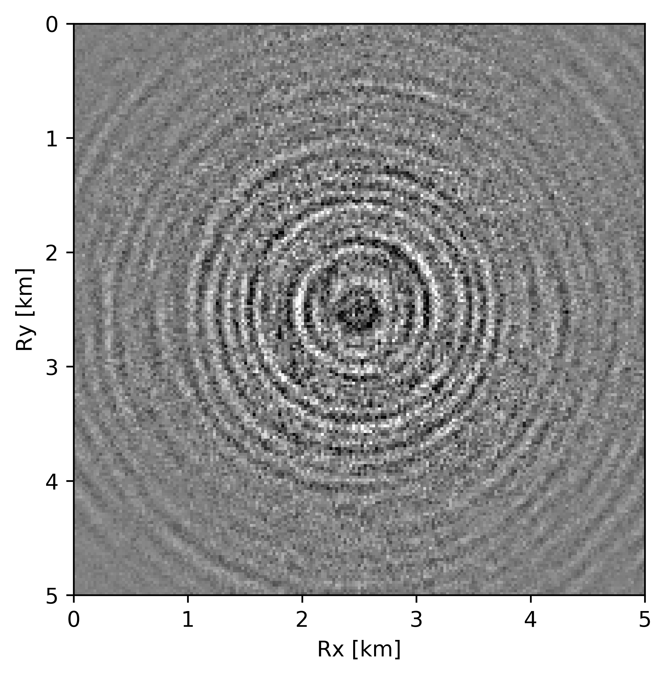
The above derivation is only valid if the above approximations involving commutations of the weight matrices with the sampling operator \(\mathcal{A}\) are sufficiently accurate. To verify that these approximations are indeed justified, we compare in Figure 7 their accuracy by comparing plots of \(\mathbf{Q}\mathcal{A}(\mathbf{Q}^{-1}\mathbf{\bar{X}W}^{-1})\) and \(\mathcal{A}(\mathbf{\bar{X}W}^{-1})\) for two different values of the weights in equations \(\ref{eqQinv}\) and \(\ref{eqWinv}\). As expected, for the small value \(w_{1,2}=0.25\) the weighting matrix \(\mathbf{Q}\) does not commute with the sampling matrix (see Figures 7a – 7c). However, for \(w_{1,2}=0.75\) the approximation is reasonably accurate (see Figures 7d – 7f). Similarly, in Figure 8 we compare plots of \(\mathcal{A}(\mathbf{Q}^{-1}\mathbf{\bar{X}W}^{-1})\mathbf{W}\) and \(\mathcal{A}(\mathbf{Q}^{-1}\mathbf{\bar{X}})\) for small and large weights. As before, for smaller weights \(w_{1,2} = 0.25\), the weighing matrix \(\mathbf{W}\) does not commute with the sampling matrix (see Figures 8a – 8c). However, for \(w_{1,2}=0.75\) the approximation is again reasonably accurate (see Figures 8d – 8f). Remember, the weights \(w_{1,2}\) reflect confidence we have in the weight matrices and are chosen small when we have confidence that the weighting matrices \(\mathbf{Q}\) and \(\mathbf{W}\) add information to the recovery. This means we need to select a value for the weights \(w_{1,2}\) that balances between how much prior information we want to invoke and how accurate the commutation relations need to be. Choosing small weights goes at the expense of large “commutation” errors while large weights leads to small “commutation” errors but limits the inclusion of the prior information via the weights.

Although, the decoupled equations \(\ref{eqwtRpar}\) and \(\ref{eqwtLpar}\) can now be parallelized over the rows of the low-rank factors \(\vector{\bar R}\) and \(\vector{\bar L}\), they come at additional computational cost. Unlike sparse observed data collected in the matrix \(\mathbf{B}\), the data matrices \(\mathbf{B}_R\) and \(\mathbf{B}_L\) are dense (have all non-zero entries) because of the multiplications by \(\mathbf{W}\) and \(\mathbf{Q}\). However, when the weights \(w_{1,2}\) are relatively large we observe that both dense matrices \(\mathbf{B}_L\), \(\mathbf{B}_R\) (Figure 9b and 9d) can be well approximated by the sparse observed data matrix \(\vector{B}\) judged by the difference plots in Figure 9. With this approximation, equations \(\ref{eqwtRpar}\) and \(\ref{eqwtLpar}\) can be solved computationally efficiently.

While the above formulation allows us to carry out weighted factored wavefield recovery in parallelized form, we observed that taking inverses of \(\mathbf{Q}\) and \(\mathbf{W}\) in the data misfit objective (see equation \(\ref{eqWeighteLRopt}\)) leads to inferior recovery because these involve reciprocals of the weights (see equations \(\ref{eqQinv}\) and \(\ref{eqWinv}\)). The value range of these reciprocals is no longer contained to the interval \((0, 1]\) and this can lead to numerical problems during the recovery. To circumvent this issue, we propose an alternative but equivalent form for the weighted formulation with weights defined as \[ \begin{gather} \label{eqparQ} \vector{\widehat{Q}} = \vector{U}\vector{U}^H + {w}_{1}\vector{U}^\perp \vector{U}^{{\perp}^{H}} = {w}_{1}\vector{Q}^{-1},\\ \label{eqparW} \vector{\widehat{W}} = \vector{V}\vector{V}^H + {w}_{2}\vector{V}^\perp \vector{V}^{{\perp}^{H}} = {w}_{2}\vector{W}^{-1} \end{gather} \] With these alternative definitions, we can as before approximate \(\mathbf{\widehat{Q}}^{-1}\mathcal{A}(\mathbf{\widehat{Q}}\mathbf{\bar{X}}\mathbf{\widehat{W}})\) by \(\mathcal{A}(\mathbf{\bar{X}\widehat{W}})\) and \(\mathcal{A}(\vector{\widehat{Q}\bar{X}\widehat{W}})\mathbf{\widehat{W}}^{-1}\) by \(\mathcal{A}(\vector{\widehat{Q}\bar{X}})\), yielding the following decoupled parallellizable equations for the factors \[ \begin{equation} \begin{aligned} \vector{\bar R}(l_1,:)^{H} := \quad & \argmin_{\vector{\bar v}} \quad \frac{1}{2} \left\|\vector{\bar v}\right\|^2 \\ & \text{subject to} \\ & \|\mathcal{A}_{l_1}(\widehat{\vector{Q}}\vector{\bar L}\vector{\bar v}) - {w_1}{w_2}\vector{B}(:,l_1)\| \leq {w_1}{w_2}\gamma \end{aligned} \label{eqwtRparv2} \end{equation} \] for \(l_1=1\cdots n\) and \[ \begin{equation} \begin{aligned} \vector{\bar L}(l_2,:)^{H} := \quad & \argmin_{\vector{\bar u}} \quad \frac{1}{2} \left\|\vector{\bar u}\right\|^2 \\ & \text{subject to} \\ & \|\mathcal{A}_{l_2}((\vector{\bar R}\vector{\bar u})^{H}\vector{\widehat{W}}) - {w_1}{w_2}\vector{B}(l_2,:)\| \leq {w_1}{w_2}\gamma \end{aligned} \label{eqwtLparv2} \end{equation} \] for \(l_2=1\cdots m\) . Equations \(\ref{eqwtRparv2}\) and \(\ref{eqwtLparv2}\) form the basis for our recovery approach summarized in Algorithm 1 below, which corresponds to \[ \begin{equation} \minim_{\vector{\bar X}} \quad \|\vector{\bar X}\|_* \quad \text{subject to} \quad \|\mathcal{A}(\vector{\widehat{Q}}\vector{\bar X}\vector{\widehat{W}}) - w_1w_2\vector{B}\|_F \leq w_1w_2\epsilon, \label{eqWeightednew2} \end{equation} \] which is equivalent to equation \(\ref{eqWeightednew}\) as we show in Appendix A.

In Algorithm 1, Line 2 corresponds to solving for each row of the low-rank factor \(\vector{\bar R}^\left(k+1 \right)\) at the \(\left(k+1 \right)^{th}\) iteration using the estimate of low-rank factor \(\vector{\bar L}^\left(k \right)\) from the \(\left(k \right)^{th}\) iteration. Similarly, Line 3 corresponds to solving for each row of the low-rank factor \(\vector{\bar L}^\left(k+1 \right)\) at the \(\left(k+1 \right)^{th}\) iteration using the estimate of low-rank factor \(\vector{\bar R}^\left(k+1 \right)\). Finally, Lines 5 and 6 correspond to retrieving the low-rank factors \(\vector{L}\) and \(\vector{R}\) from \(\vector{\bar L}\) and \(\vector{\bar R}\), respectively.

Case studies

We now conduct a series of experiments to evaluate the accuracy of the proposed weighted wavefield reconstruction methodology. In all cases, we have access to the ground truth fully sampled data. This allows us to assess the accuracy by means of visual inspection and S/R’s (Signal to noise ratio). Our examples include the seismic line from the Gulf of Suez we discussed earlier and a complex full-azimuth synthetic 3D dataset.

Gulf of Suez field data: 2D example

To evaluate the performance of our recursively weighted wavefield recovery method on field data, we conduct an experiment on a 2D line from the Gulf of Suez. The fully sampled split-spread dataset consists of \(1024\) time samples, acquired with \(354\) sources and \(354\) receivers. Time is sampled at \(0.004\, \mathrm{s}\). The source-receiver spacing is \(25\, \mathrm{m}\). To test our algorithm, we reconstruct this 2D line from randomly subsampled traces, which we obtain by removing \(75\%\) of the sources via optimal jittered subsampling (F. J. Herrmann and Hennenfent, 2008).

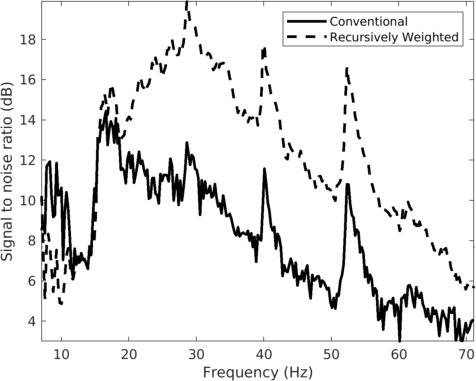
We assess the performance of recursively weighted matrix factorization by comparing wavefield recovery with and without weighting as a function of the angular frequency. To avoid the impact of noise at the low frequencies, we start the recovery at \(7.0\, \mathrm{Hz}\). Since this is a small problem, we reconstruct the frequency slices by performing \(150\) iterations of the SPG-LR algorithm (Van Den Berg and Friedlander, 2008; A. Aravkin et al., 2014) for each frequency. We compare wavefield reconstructions with and without weights the results of which are summarized in Figure 10. From these results we can see that above \(17\)Hz, the wavefield reconstruction clearly benefits from including weights for reconstructions carried out with the same number of iterations but without weighting.

For comparison purposes, we also reconstruct missing data using the conventional matrix factorization method. For fairness of comparison, we once again use \(150\) iterations of SPG-LR algorithm for each frequency slice. As expected other than few lower frequency slices where conventional method performs well, we get improvements in signal to noise ratio (Figure 10) across all other frequency slices with our recursively weighted approach.

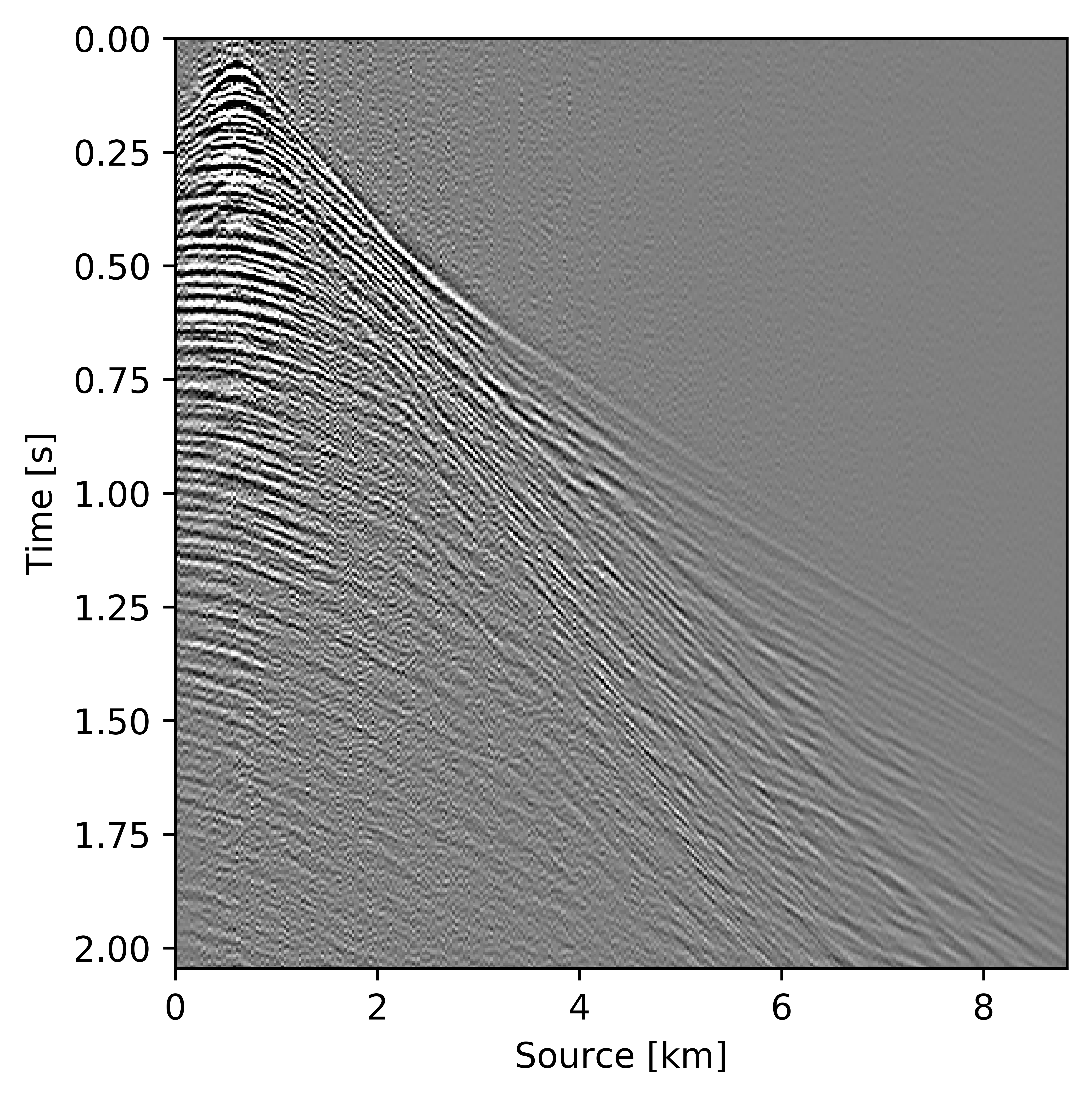
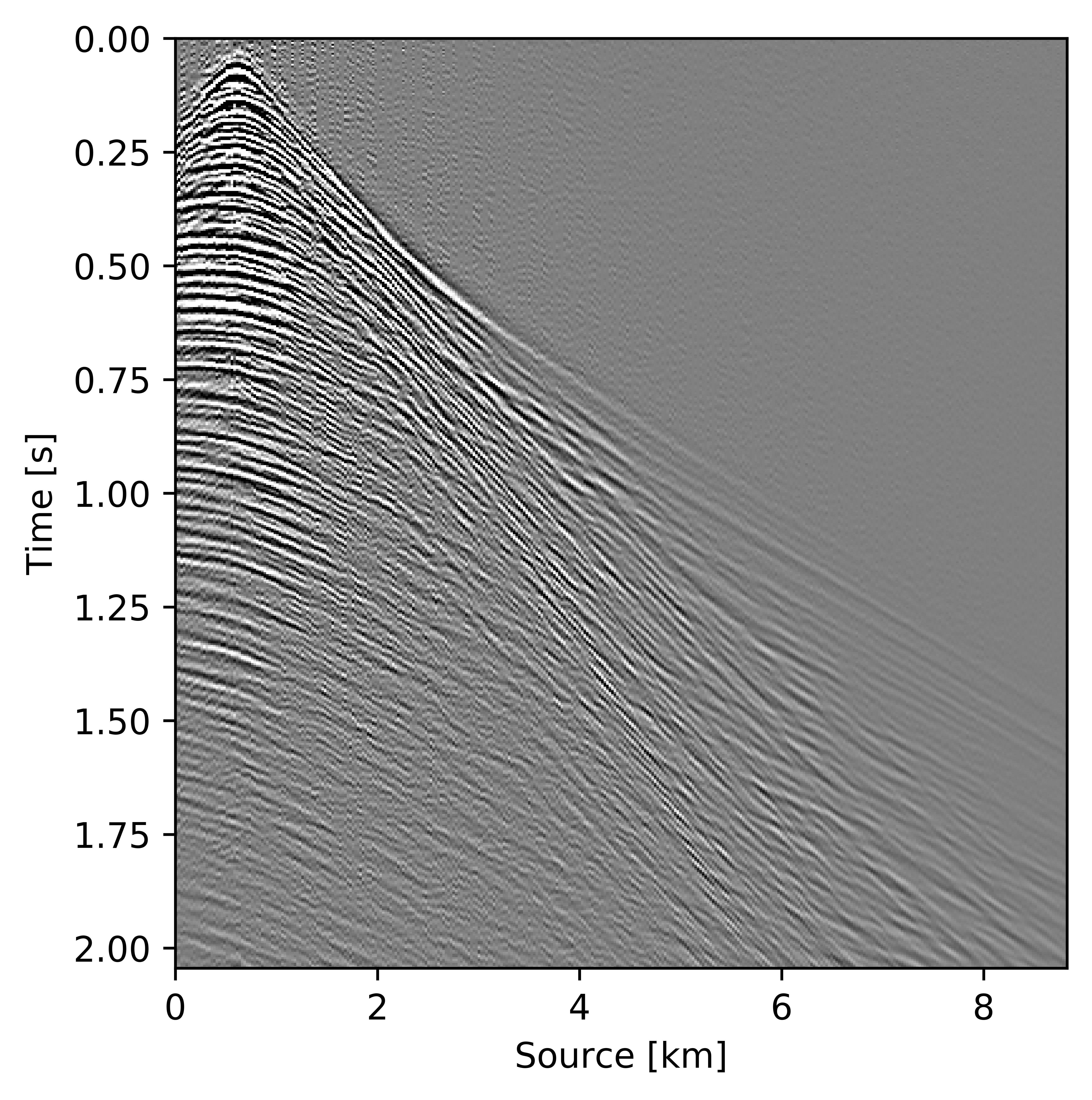
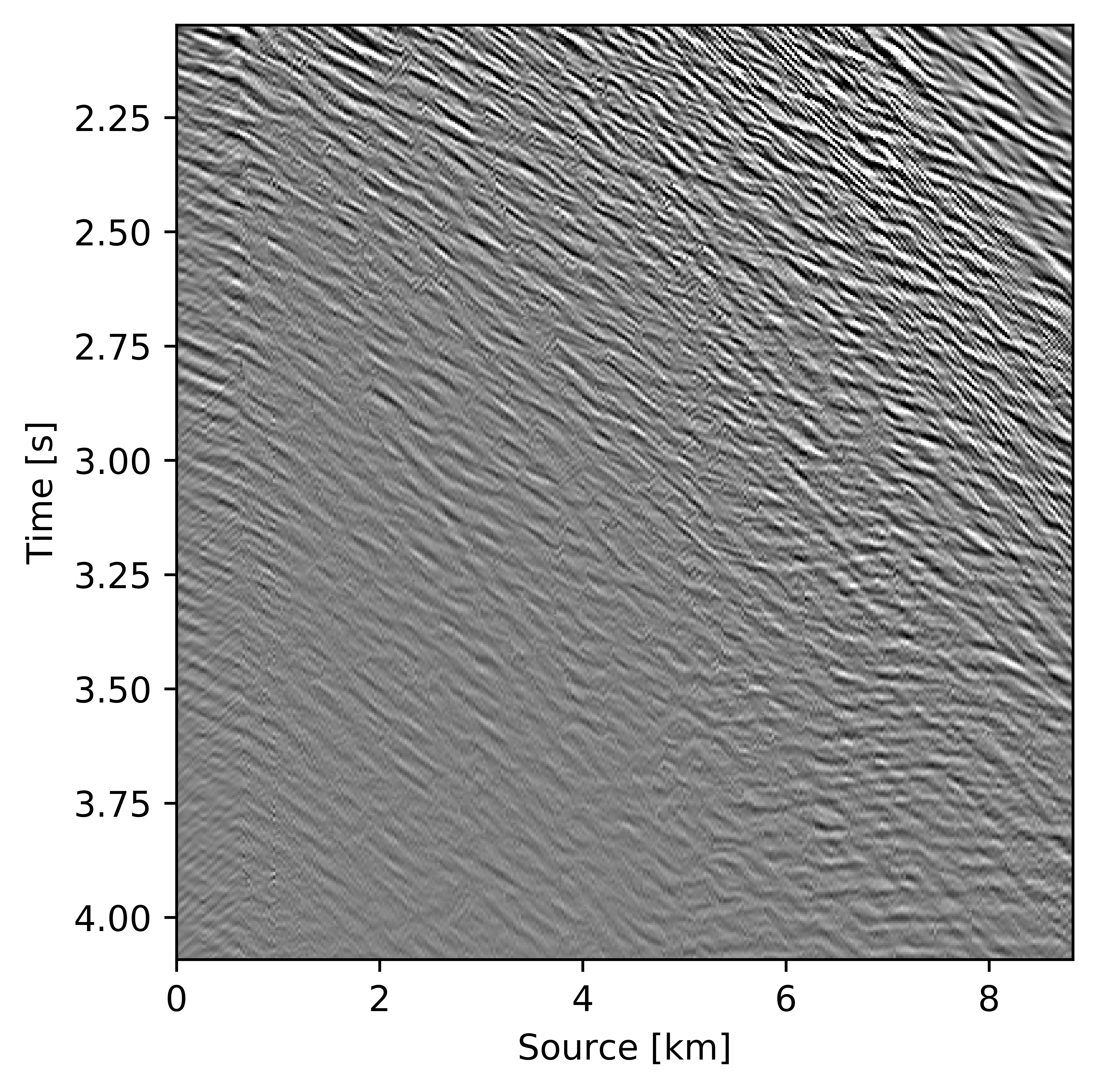
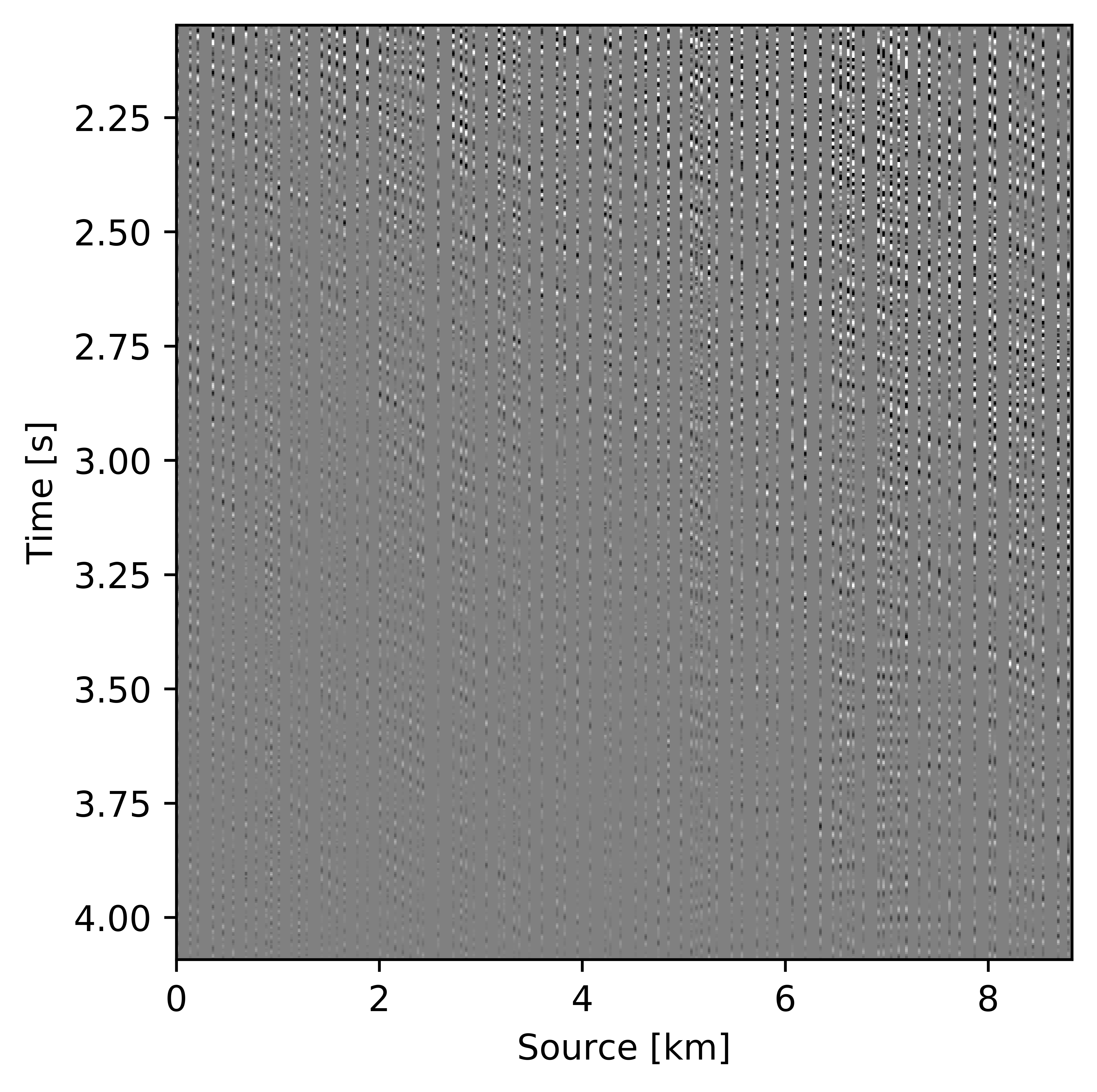
Figures 11c and 12c include the shallow and deeper parts of a reconstructed common receiver gather extracted from results based on the conventional method yielding \(S/R = 6.9\, \mathrm{dB}\). In the data residual plots (Figures 11d and 12d), we observe signal leakage and noise due to reconstruction artifact in both shallow and deeper parts. By signal leakage we mean that there are coherent events in the data residual plot indicating incomplete reconstruction of data. Also, at far offsets we observe signal leakage in the difference plot. Far offset data is important for FWI (Full Waveform Inversion) purposes since it contains turning waves. On the other hand, we observe better reconstructed data in the common receiver gather (Figures 11e and 12e) extracted from reconstructed data using the recursively weighted approach with improved \(S/R\) of \(11.7\, \mathrm{dB}\). Its corresponding data residual plot (Figures 11f and 12f) shows less signal leakage in comparison to its conventional counterpart. Even at far offsets, we observe better reconstruction of signal.

Synthetic Compass model data: 3D example

In 2D seismic surveys, receivers only measure wavefields traveling in the vertical plane along sources and receivers. Therefore, we fail to capture reflections out of the 2D source-receiver plane. This lack of recording of out of plane scattering ultimately affects the quality of the subsurface image, especially in regions where there is strong lateral heterogeneity. To capture 3D effects most of the seismic exploration surveys are 3D nowadays during which sources and receivers are spread along the surface rather than confined to a single line. To evaluate the performance of our recursively weighted low-rank matrix factorization methodology in this more challenging 3D setting, we consider synthetic 3D data simulated on the Compass model (E. Jones et al., 2012). We choose this model because it contains velocity kickbacks, strong reflectors, and small wavelength details constrained by real well-log data collected in the North Sea. Because of the complexity of this dataset, which mimics marine acquisition with a towed array, we face similar challenges in wavefield reconstruction as we would face dealing with real 3D field data. The authors Da Silva and Herrmann (2015) also used this 3D dataset to evaluate their tensor-based wavefield reconstruction algorithm based on the Hierarchical Tucker decompositions.

For this experiment, we use a subset of the total data volume of \(501 \times 201 \times 201 \times 41 \times 41\) gridpoints—i.e., \(n_t \times n_{rx} \times n_{ry} \times n_{sx} \times n_{sy}\) along the time, receiver \(x\), receiver \(y\), source \(x\), and source \(y\) directions. Here, \(n_t\) is the number of samples along time, \(n_{rx}\), \(n_{ry}\) are number of receivers along \(x\) and \(y\) directions respectively and \(n_{sx}\), \(n_{sy}\) are number of sources along \(x\) and \(y\) directions respectively. In both spatial directions, the spacing between the adjacent sources is \(150.0\, \mathrm{m}\) and \(25.0\, \mathrm{m}\) between adjacent receivers. The sampling interval along time is \(0.01\, \mathrm{s}\). To get the subsampled data, we remove \(75\%\) of the receivers from jittered locations (F. J. Herrmann and Hennenfent, 2008). We use this incomplete data as input to our recursively weighted wavefield reconstruction scheme.

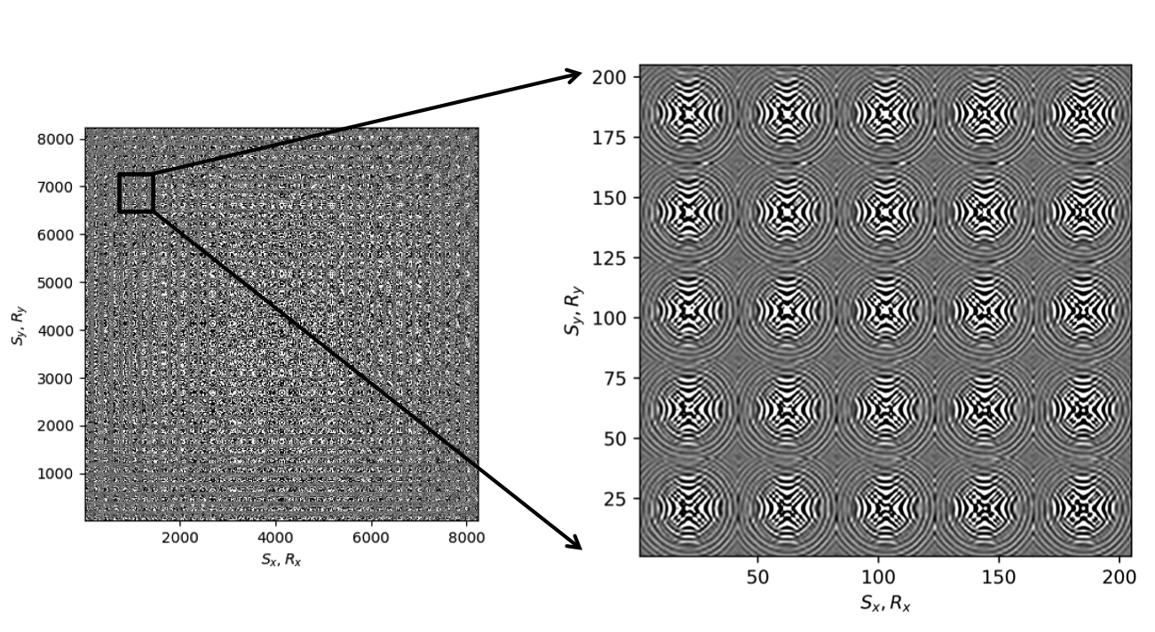
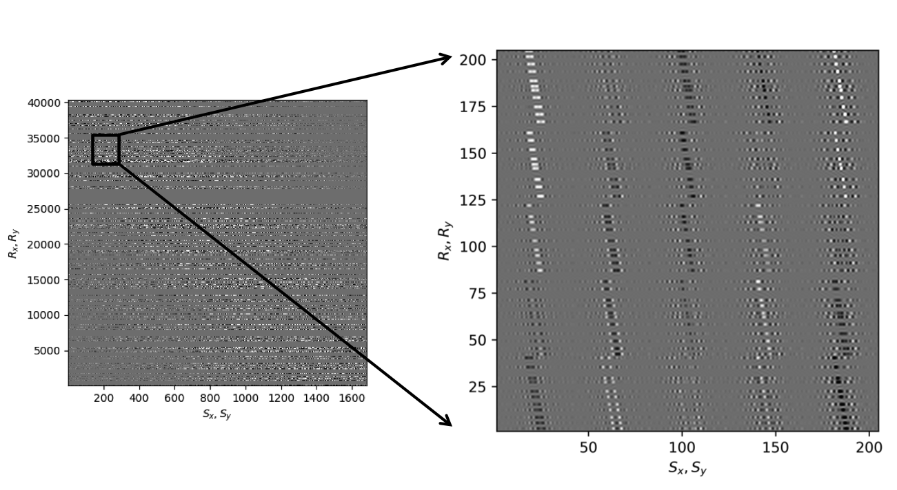
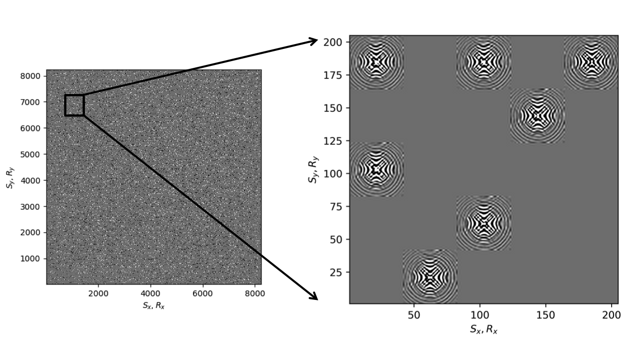
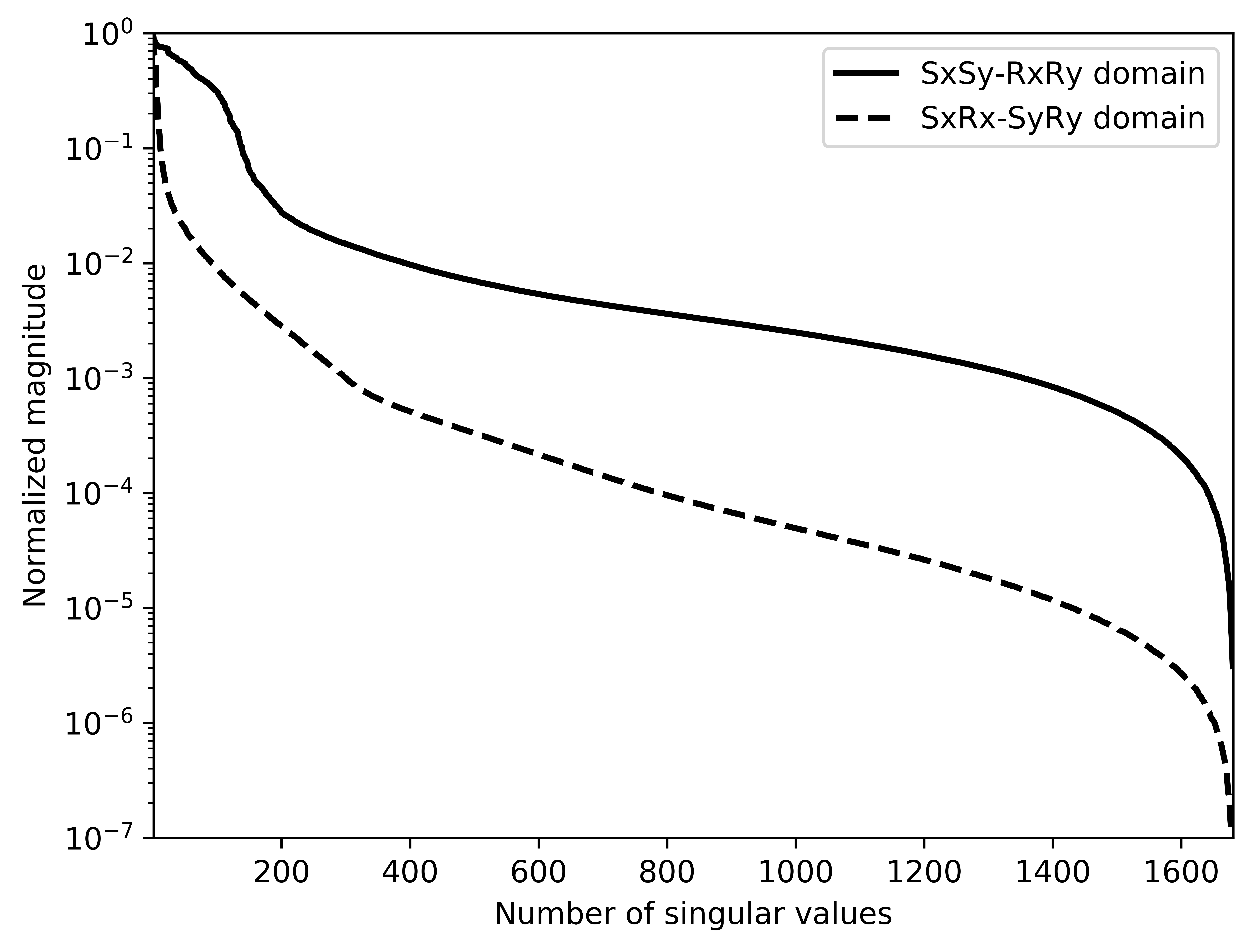
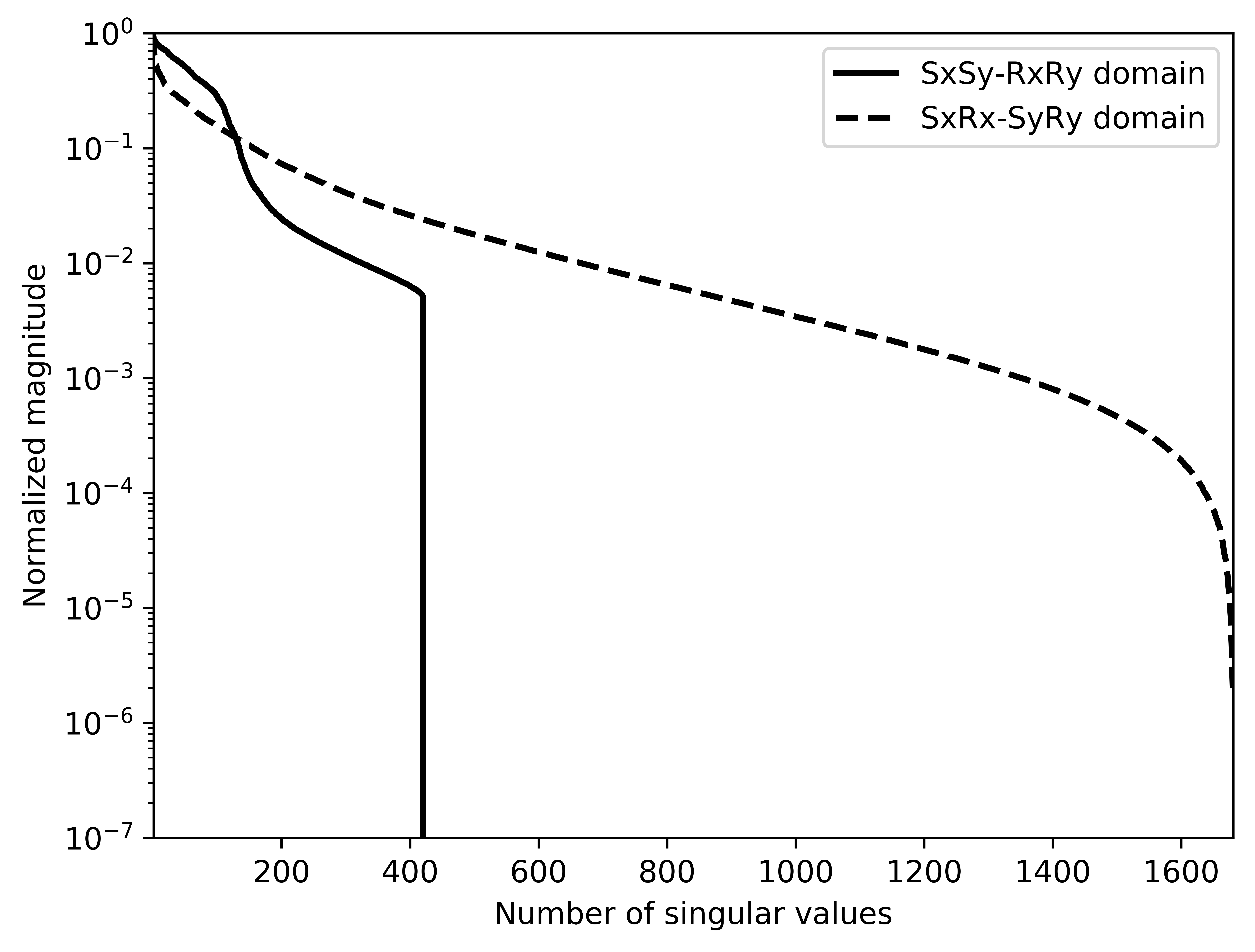
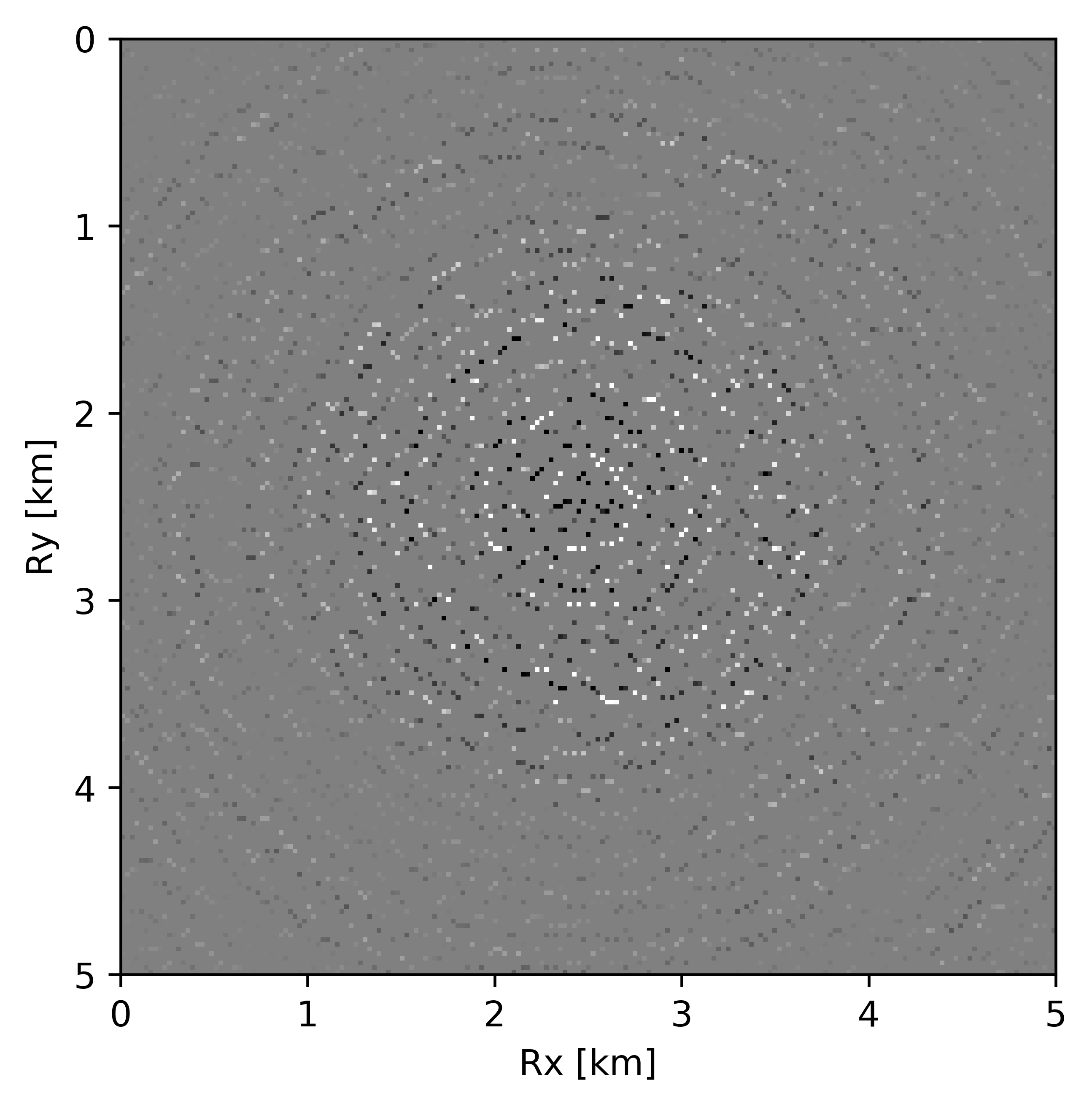
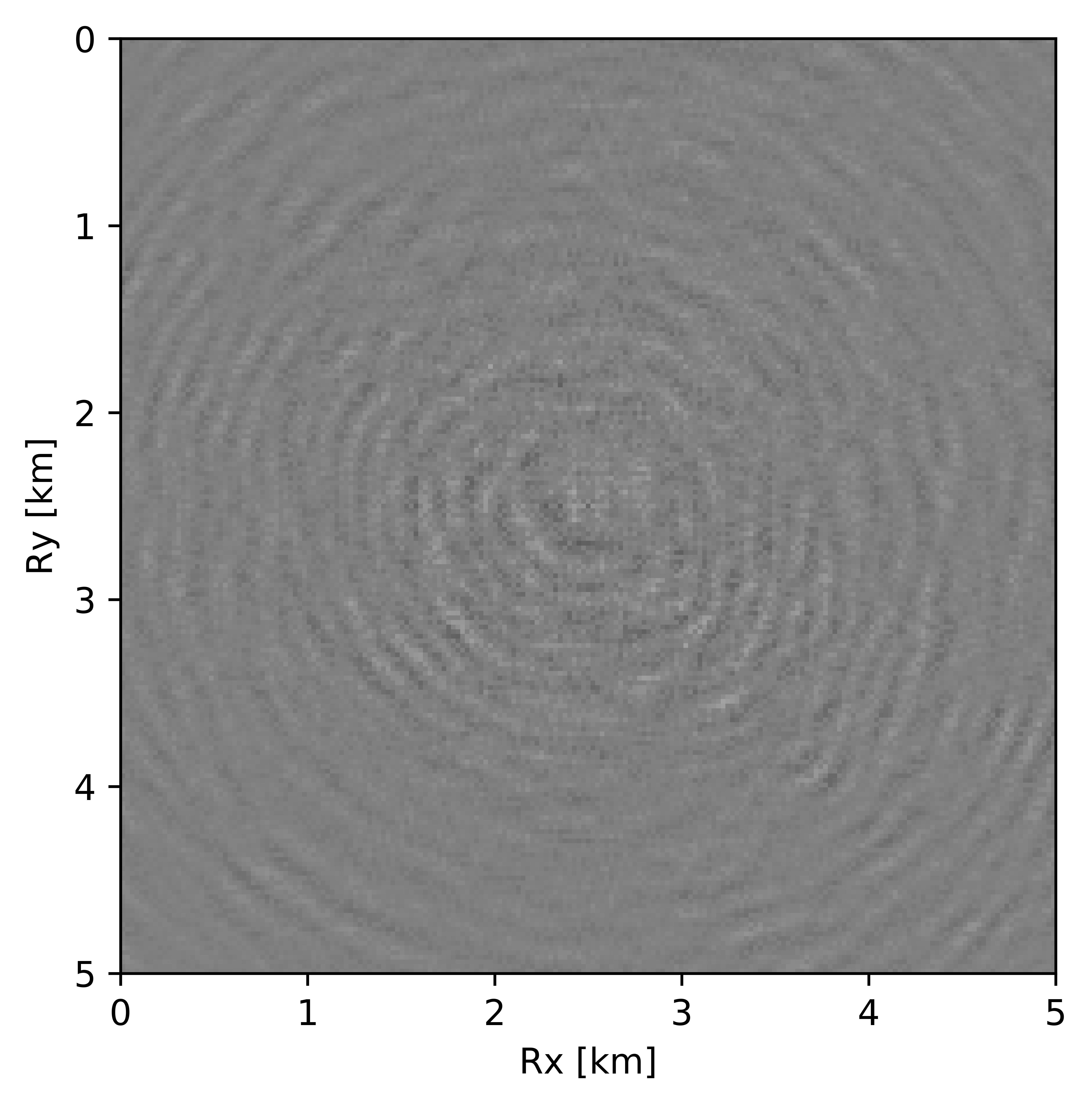
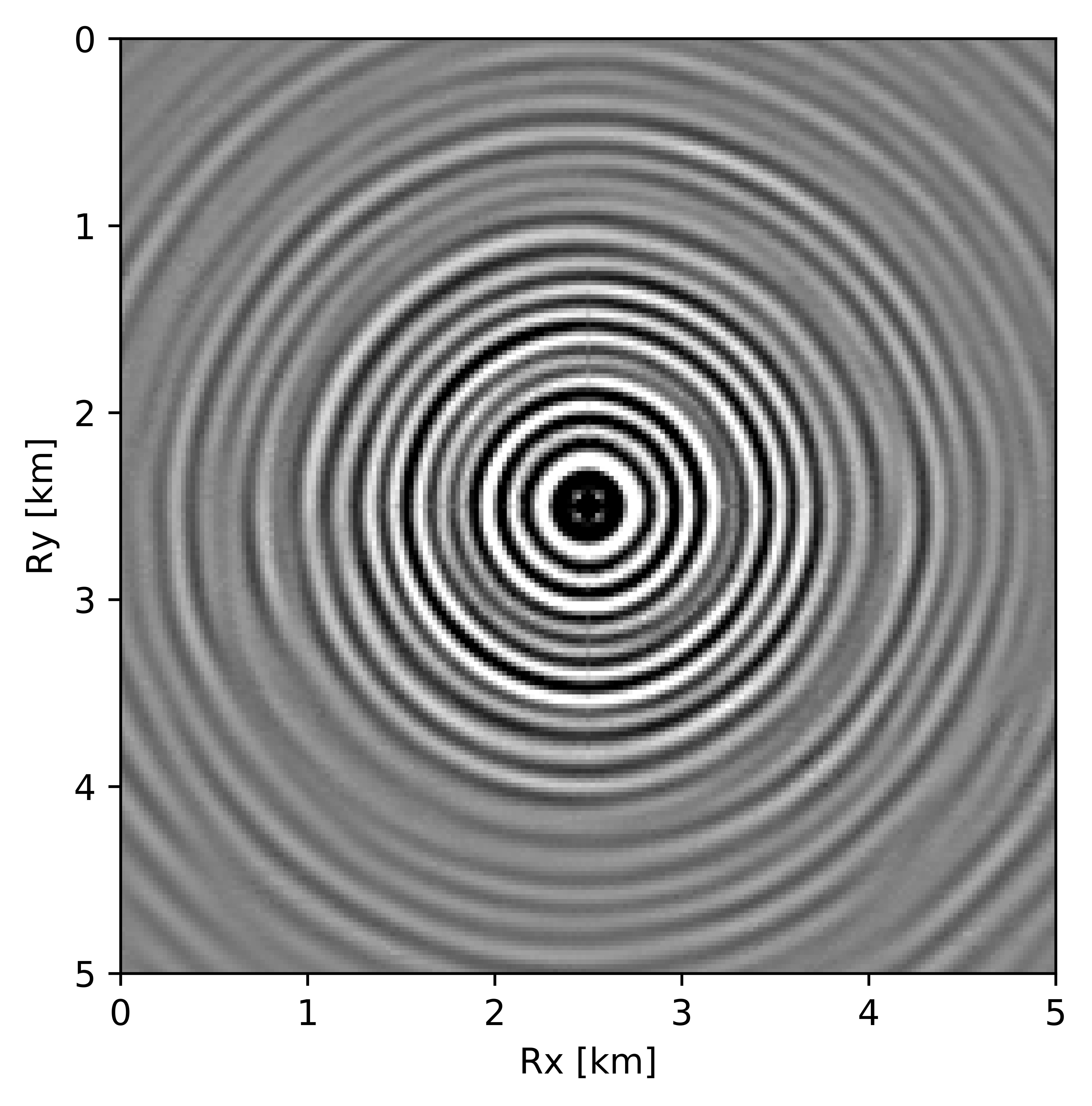
Before proceeding further, let us first briefly discuss the organization of the data in which we will carry out the wavefield reconstructions. While we could in principle transform the data into the midpoint offset domain as in the 2D case, we follow Da Silva and Herrmann (2015) and Demanet (2006) and exploit the fact that monochromatic 3D frequency slices rearranged along the \(x\) and \(y\)-coordinates for sources and receivers can be well approximated by a low-rank factorization. In this rearrangement the data is organized as a matrix with \({S}_{x}, {R}_{x}\) and \(S_y, R_y\) coupled along the columns and rows respectively unfolded along is coordinate directions. Here \(S_{x,y}\) and \(R_{x,y}\) are the source and receiver coordinates along the \(x\) and \(y\) directions. After rearrangement in this non-canonical form, the frequency slices are low-rank while data with randomly missing receivers is not (juxtapose \(10.0\, \mathrm{Hz}\) frequency slices in Figures 13c and 13d and the singular value plots in Figures 14a and 14b). We choose \(10\, \mathrm{Hz}\) frequency slice as the changes in the rate of decay of singular values upon sampling at lower frequencies is more prominent in comparison to changes we observe at higher frequencies. This frequency choice allows us to better demonstrate the reasoning behind choosing \({S}_{x}, {R}_{x}\) and \(S_y, R_y\) domain for reconstruction. In the canonical organization, missing receivers leads to missing rows and this decreases the rank (cf. solid lines in Figure 14) in the non-canonical rearrangements the rank increases (cf. dashed lined in Figure 14). The sudden drop in the singular values in the canonical arrangement is a direct consequence of the fact that removing complete rows or columns decreases the rank. From the behavior of the singular values before and after removal of the receivers, it is clear that the simple rearrangement of the data in the non-canonical organization can serve as the transform domain in which to recover that data via weighted low-rank factorization.

As before, we now perform the full-azimuth 3D wavefield reconstruction for each frequency slice using our proposed recursively weighted low-rank matrix factorization approach. Since this is a relatively large problem, we employ the parallel framework presented in the previous section (Algorithm 1) for \(4\) alternations with \(40\) iterations of SPG-\(\ell_2\) per frequency slice. We choose these values because for a given rank parameter we observed better continuity of signals and lesser noise in the reconstructed data. In addition to setting the number of alternations, i.e. switching between Equations \(\ref{eqwtRparv2}\) and \(\ref{eqwtLparv2}\), the algorithm needs us to specify the rank of the factorization and the weights. Based on tests performed using different rank values and weights, we selected a rank of \(r=228\) and a value for the weights of \(w_{1,2}=0.75\), because they provide a good balance between quality of reconstructed data (in terms of continuity of events, lesser noise) and computational time.

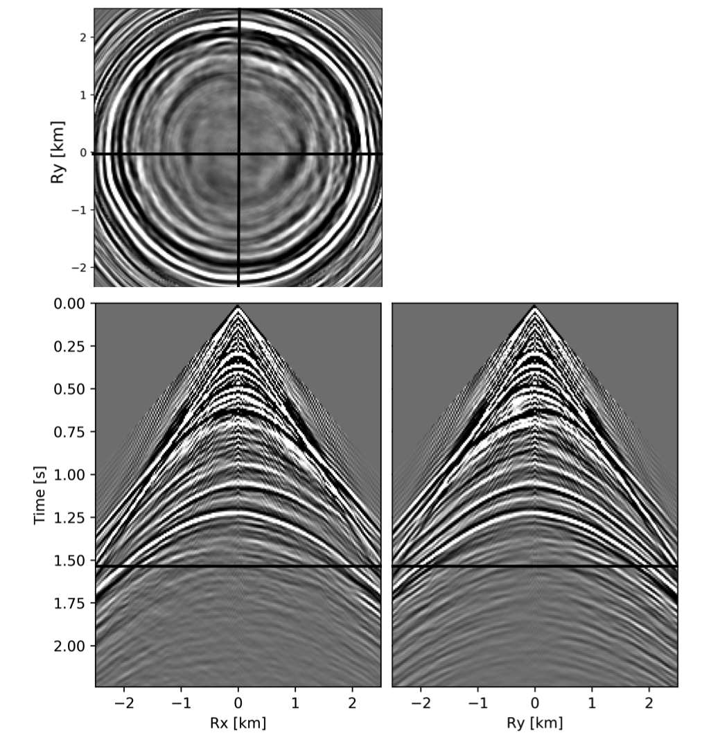
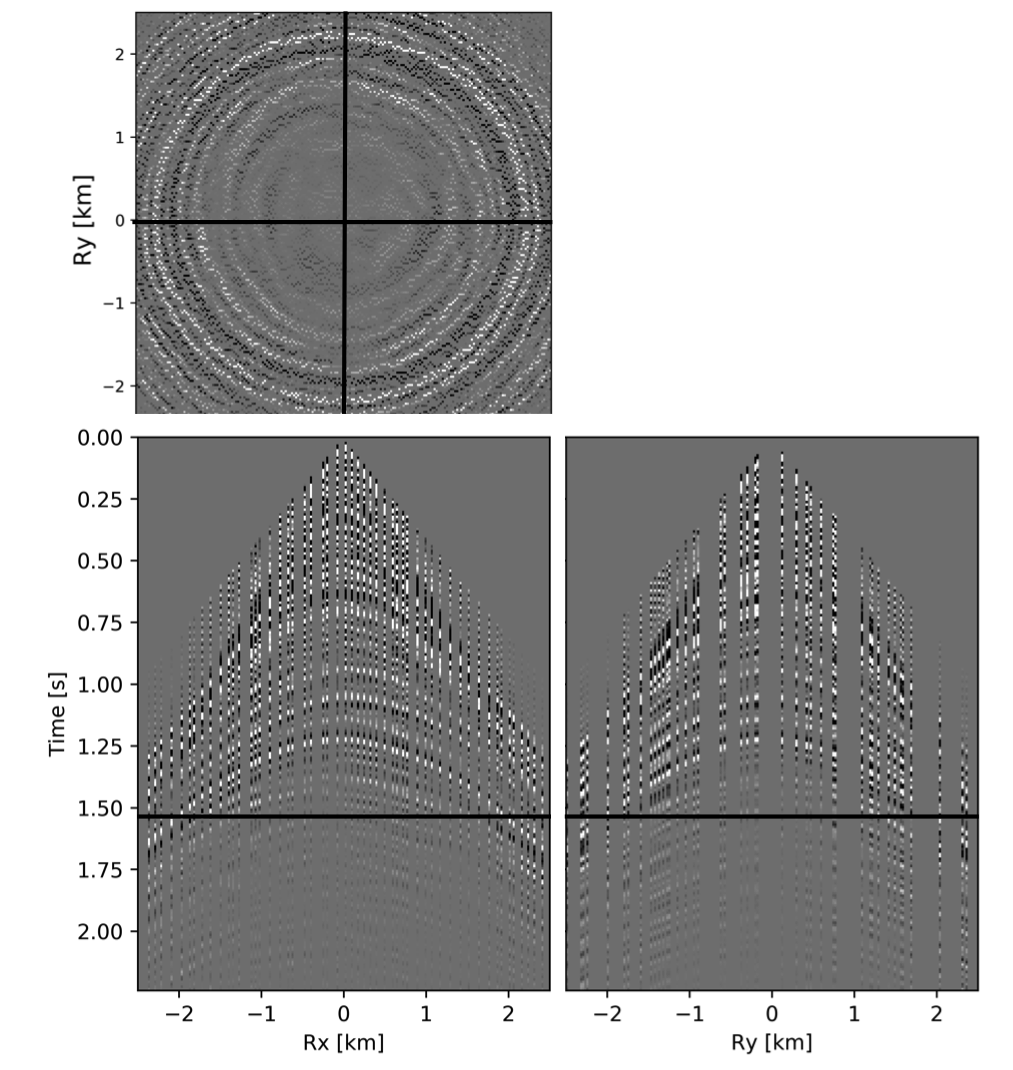
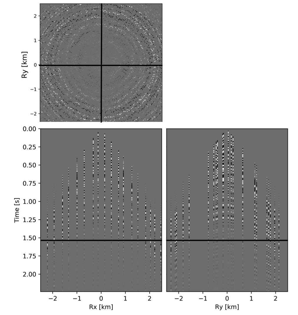
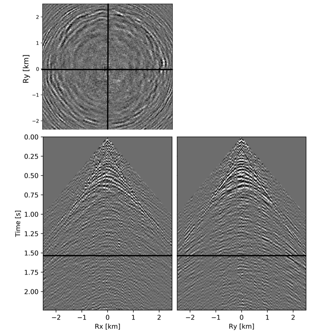
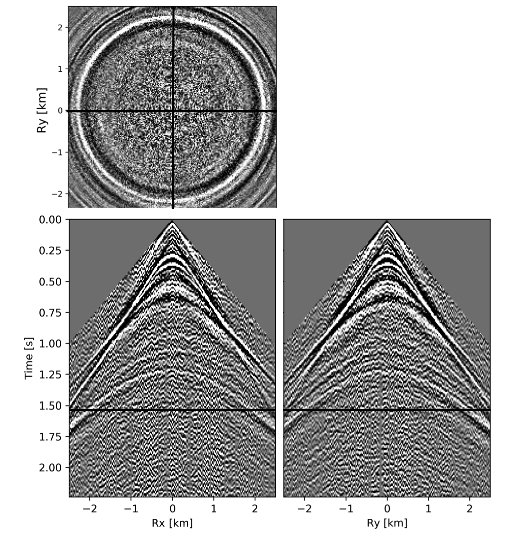
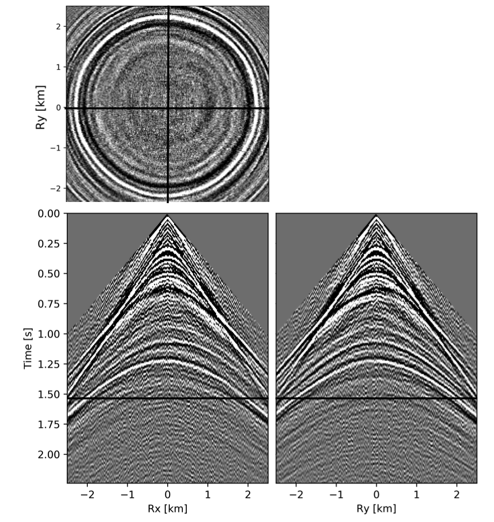
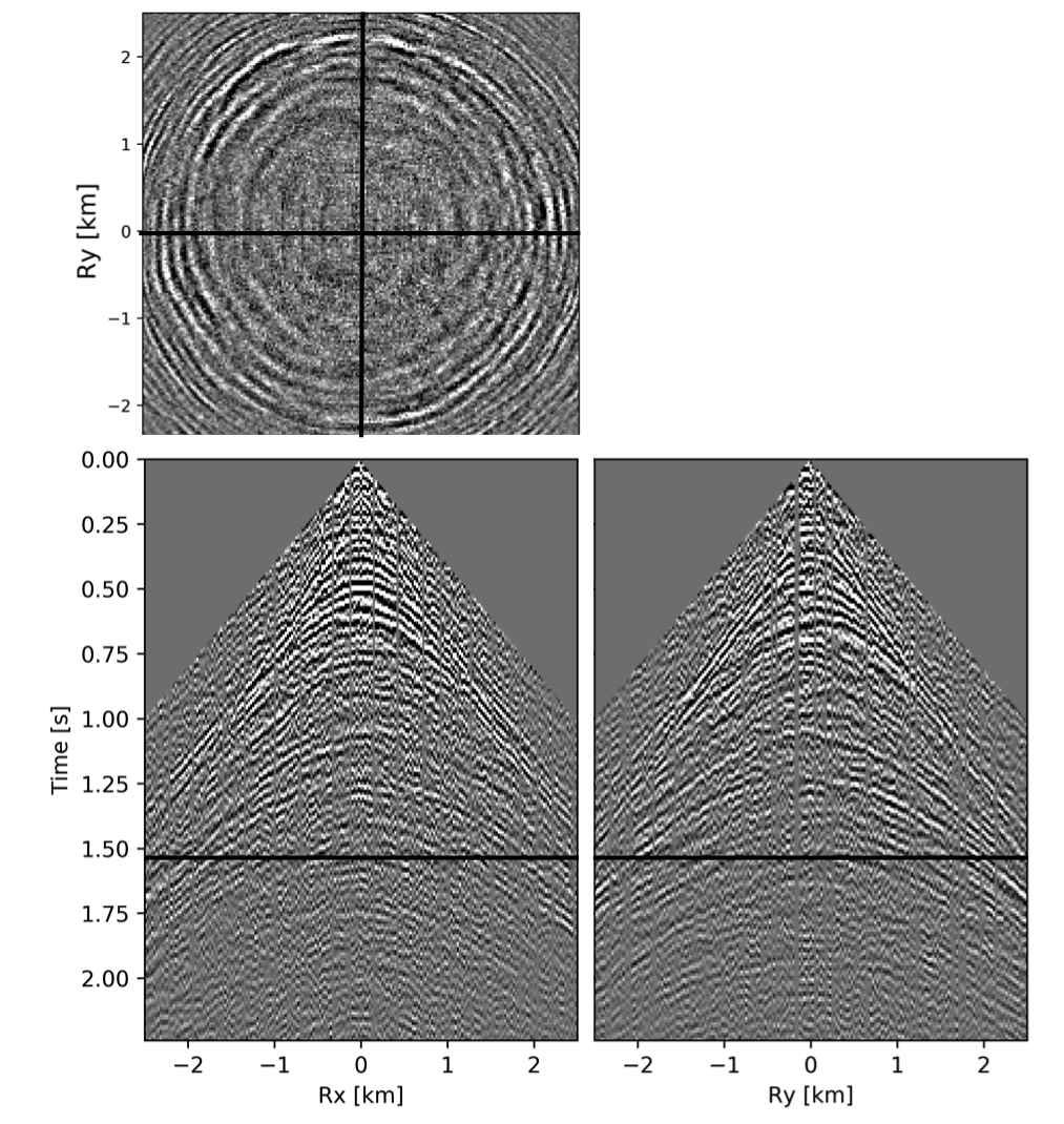
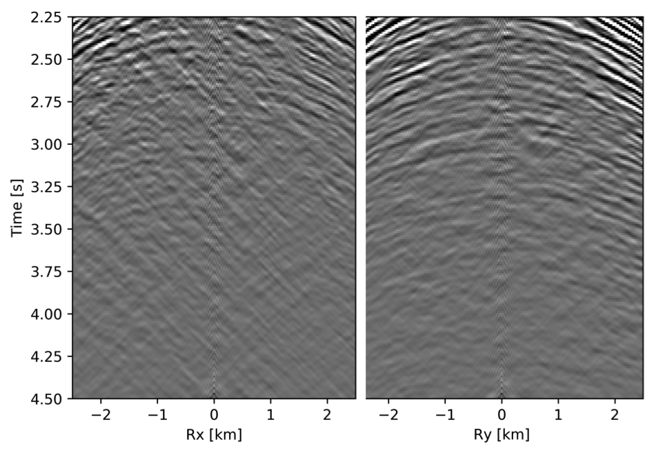
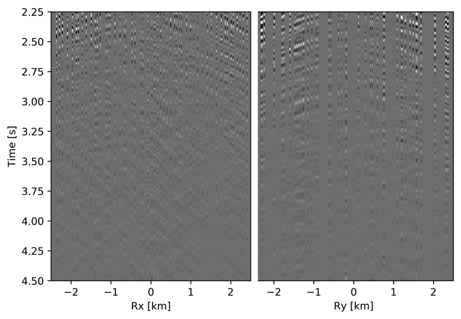
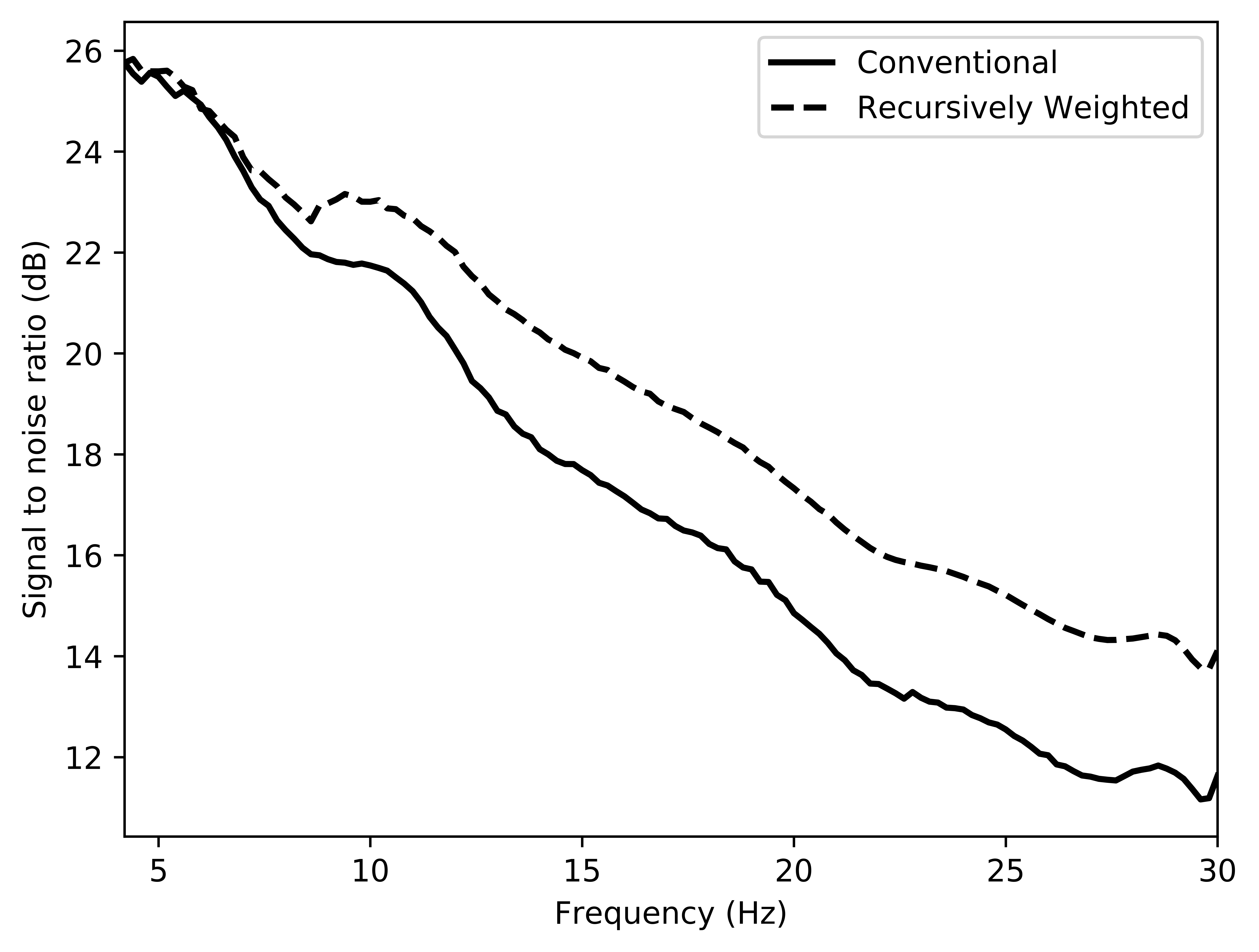
To avoid noise at the very low frequencies observed due to simulation artifacts, we start our recursively weighted from \(4.4\, \mathrm{Hz}\). For comparison, we also use conventional matrix completion for wavefield reconstruction. Here, we use the same number of alternations and SPG-\(\ell_2\) iterations as before. We also use same rank of \(228\). For visualization purpose we show results in a common shot gather (Figure 15a) extracted from \(15\, \mathrm{Hz}\) frequency slice. Here we choose higher frequency of \(15\, \mathrm{Hz}\) instead of \(10\, \mathrm{Hz}\) to show how the recursively weighted method is able to give better reconstruction at high frequency in comparison to reconstructed data obtained from the conventional method. In Figure 15b we show subsampled shot gather with \(75 \%\) missing receivers. Using the conventional method we get S/R of \(17.7\, \mathrm{dB}\) for the reconstructed data at \(15.0\, \mathrm{Hz}\) (Figure 15d). Whereas, with the recursively weighted method we get improved S/R of \(19.9\, \mathrm{dB}\) (Figure 15f). We also observe less leakage of signal and less noise in the residual plots for the data reconstructed using recursively weighted method (Figure 15g) in comparison to the data reconstructed using the conventional method (Figure 15e). From Figure 18a, we also observe improvement in the S/R of reconstructed data for all the frequencies with the recursively weighted method (dashed black line in Figure 18a) in comparison to its conventional counterpart (solid black line in Figure 18a). In Figures 16 and 17 we also show comparison of the recursively weighted and conventional method in time domain common shot gather at earlier and later arrivals respectively. In Figure 16, we also show comparison of a time slice at \(1.6\, \mathrm{s}\) extracted from a 3D common shot gather. Figure 16a shows two common shot gathers extracted from the true data along \(x\) and \(y\) directions along with a time-slice on top left corner. Figure 16b shows the corresponding observed data with missing receivers. We observe improved reconstruction of signals in the common shot gather (with \(S/R = 17.8\, \mathrm{dB}\)) reconstructed from recursively weighted method (Figure 16f) in comparison to the reconstructed data from the conventional method (Figure 16d) with \(S/R\) of \(15.3\, \mathrm{dB}\). Even in the residual plots we observe less leakage of signal with the recursively weighted method (Figure 16g) in comparison to its conventional counterpart (Figure 16e). In Figures 17a and 17b, we show the same common shot gather at later time along \(x\) and \(y\) directions extracted from true and observed data respectively. We observe noise in the data and corresponding residual (Figures 17c and 17d) reconstructed from the conventional method. Whereas, we observe better reconstruction and less noise in the data reconstructed (Figures 17e and 17f) from the recursively weighted method.

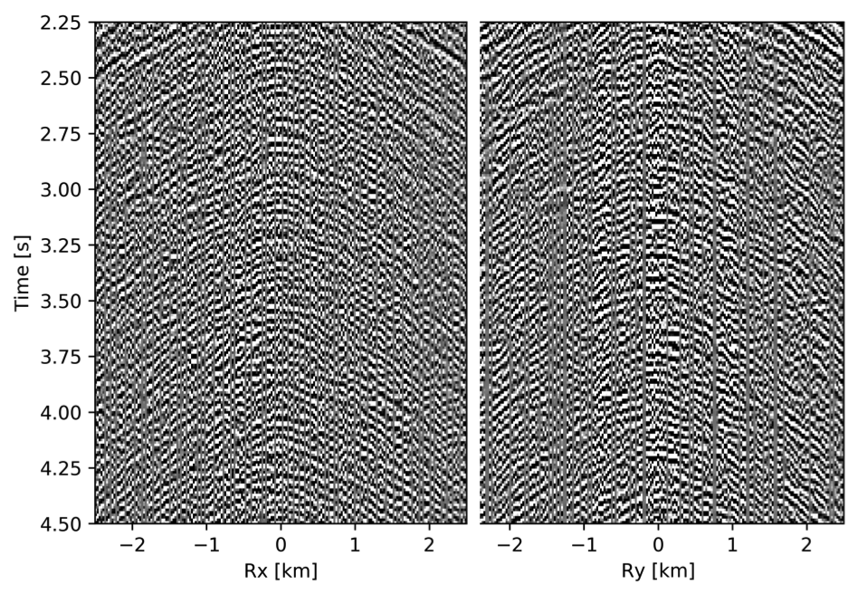
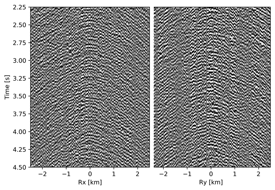
BG synthetic 3D data with \(90 \%\) missing receivers

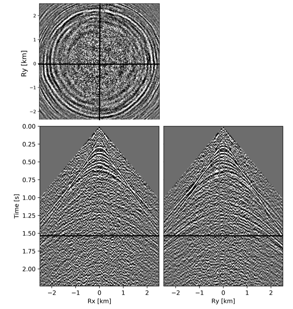
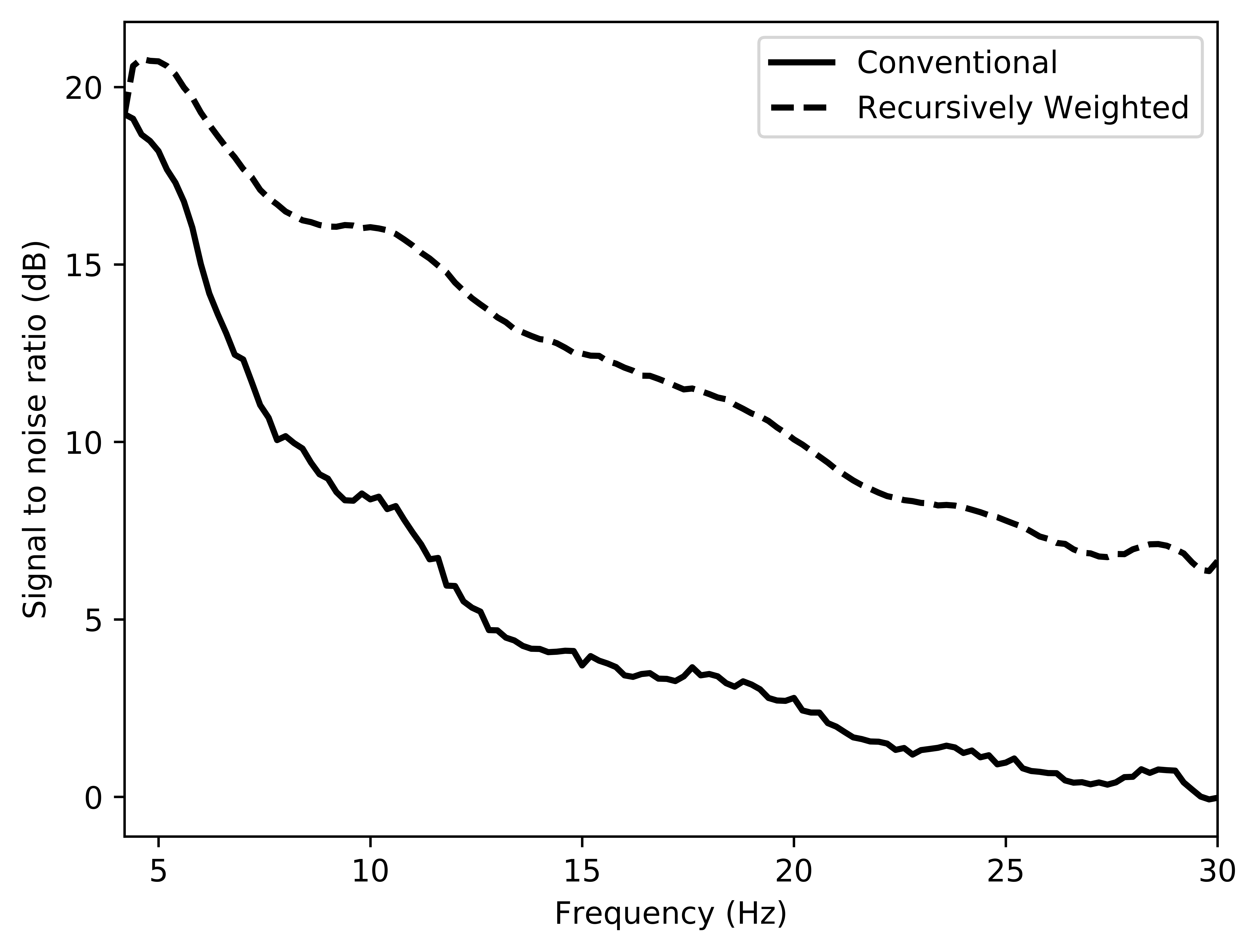
Next we test the ability of the recursively weighted method with a reduced number of samples. We subsample the BG synthetic 3D data by \(90\%\) using jitter subsampling, i.e. we use only \(10\%\) of receivers for wavefield reconstruction. We use \(4\) alternations and \(40\) inner iterations of SPG-\(\ell_2\) in each alternation per frequency slice for both conventional and recursively weighted method. We use rank parameter of \(228\) for all the frequency slices. Like before we arrive at these values by inspecting the quality of reconstructed data based on the continuity of signal and attenuated noise in the reconstructed data. To avoid noise at lower frequencies we start recursively weighted method from \(4.4\, \mathrm{Hz}\). As evident from the signal to noise ratio plot (Figure 18b), we observe improvement in data reconstruction quality across all the frequency slices using the recursively weighted method (dashed black line in Figure 18b) in comparison to its conventional counterpart (solid black line in Figure 18b). In a common shot gather extracted from a frequency slice at \(15\, \mathrm{Hz}\), we observe better continuity and less noise in the reconstructed wavefield (Figure 15j) in comparison to the reconstruction obtained from its conventional counterpart (Figure 15h). We observe more leakage of signal in the data residual with the conventional method (Figure 15i) in comparison to the data residual obtained from recursively weighted method (Figure 15k). In Figure 16 we compare data reconstruction in time domain using conventional (Figures 16h and 16i) and recursively weighted method (Figures 16j and 16k). We again observe better data reconstruction and reduced data residual with the recursively weighted method in comparison to reconstruction obtained from the conventional method.

Discussion

From the above case studies it is clear that recursively weighted low-rank matrix completion provides several benefits over conventional method. The reconstructed data preserves the signals and continuity of events even at high frequencies and at deeper sections where amplitude is very weak. We arrive at these results by exploiting the fact that fully sampled seismic data can be approximated by a low-rank matrix in some transform domain and randomized/jittered sampling degrades (or negatively affects) this low-rank property. We also exploit the fact that there is some degree of similarity between the subspaces of adjacent frequency slices of the seismic data.

Our method, which uses recursively weighted low-rank matrix completion, outperforms its conventional counterpart in terms of quality of the reconstructed data specially at higher frequencies. At higher frequencies conventional low-rank matrix completion performs poorly because these increasingly complex matrices eventually violate our low-rank assumption. As we mentioned earlier, good quality high frequency content in the data is important for high-resolution imaging of earth’s subsurface and also for inversion of earth’s physical parameters with fine details.

Weighted matrix completion was first introduced by A. Aravkin et al. (2014) to improve the seismic data reconstruction quality of the conventional matrix completion framework. Here we have exploited the potential of weighted method by recursively reconstructing data from low to high frequencies. Also, we have made the original weighted method formulation proposed by A. Aravkin et al. (2014) computationally efficient by switching the weights from objective to data misfit constraint function.

Similarity between the adjacent frequency slices and appropriate choice of weights play key role in the success of recursively weighted method. Conventional method is easily parallelized over frequencies making it computationally very efficient. Whereas, the interdependence between frequency slices in the recursively weighted method does not allow us to parallelize the recursively weighted method over frequencies. This poses computational challenge especially for large scale 3D datasets. By using the strategies of alternating minimization and decoupling we have made the recursively weighted method computationally efficient for higher weights. Depending on the availability of computational resources, the recursively weighted method can be efficiently applied to large scale 3D datasets. Our parallel weighted framework partially exploits the benefits of weighted low-rank matrix factorization since it can be parallelized only for higher weights. Despite this, our numerical experiments demonstrate improvements in the reconstructed data quality across all the frequencies for 3D seismic data generated on a geologically complicated velocity model resembling part of true Earth’s subsurface. To exploit the full benefits of weighted method for large 3D datasets, our future work will focus on extending this methodology to exploit parallelism even for smaller weight values.

By directly using the low-rank factors from a subsequent previous frequency slice to calculate the weight matrix, our recursively weighted framework avoids taking SVDs of the complete dataset to calculate its row and column subspaces. Our SVD free parallel weighted framework can be applied to industry scale large seismic datasets. With the advent of cloud computing there are plenty of computational resources available. But the main issue is to use these resources to optimize both the turnaround time and the budget. Therefore, next steps will be to re-engineer the weighted framework to efficiently use the cloud based computational resources using the ideas of serverless computing. For example, Witte et al. (2019) designed serverless computing architecture to perform large scale 3D seismic imaging.

Both the datasets used for experiments have sources and receivers on a uniform grid but in reality this is not the situation. Because of environmental and operational constraints sources and receivers are often shifted from the uniform grid. If we do not take into account of this shift in our reconstruction framework then we can encounter poor performance of the reconstruction framework. By incorporating an extra operator (Lopez et al., 2016) corresponding to these shifts from the uniform grid we can apply our weighted framework to field data recorded on a non-uniform grid.

Conclusions

While successful at the low to midrange frequencies, wavefield reconstruction based on matrix factorization fails at the higher frequency where seismic data is no longer low rank. We overcome this problem by exploiting similarities between low-rank factorizations of adjacent monochromatic frequency slices organized in a form that reveals the underlying low-rank structure of, the for budgetary and physical reasons not accessible, fully sampled data. During matrix factorization these similarities take the form of alignment of the subspaces in which the low-rank factors live. By introducing weight matrices that project these factors onto the nearby subspace of the adjacent frequency, the performance of the low-rank matrix factorization improves if this beneficial feature is used recursively starting at the lower frequencies. However, turning this approach into an algorithm that scales to industry-scale wavefield reconstruction problems for full-azimuth data requires a number of additional important steps. First, we need to avoid costly projections onto weighted constraints. We accomplish this by moving the weights to the data misfit. This simple reformulation results in an equivalent formulation, which is computationally significantly faster. Secondly, while the recursively applied weighting matrices improve the performance for the high frequencies, the introduction of these matrices does not allow for a row-by-row and column-by-column parallelization of the alternating minimization procedure we employ to carry out the matrix factorizations on which our low-rank wavefield reconstruction is based. We overcome this problem by balancing the emphasis we put on information from adjacent frequency slices with our ability to decouple the operations so that the algorithm can be parallelized. By means of carefully selected examples on a 2D field dataset and on a full-azimuth 3D dataset, we demonstrate the ability of the proposed algorithm to handle high frequencies. We also show that the proposed algorithm scales well to 3D problems with large percentages of traces missing. From these results, we argue that the proposed approach could be a valuable alternative to transform-based methods that are force to work on small multidimensional patches.

Acknowledgment

First and second authors have equal contribution to this paper. This research was funded by the Georgia Research Alliance and the Georgia Institute of Technology.

Appendix A

In this section, we justify our parallel implementation of the weighted matrix completion problem. Beginning at equation \(\ref{eqWeighted}\), our original weighted program, we will arrive at equations \(\ref{eqwtRparv2}\) and \(\ref{eqwtLparv2}\) which specify our implemented parallel counterpart.

Recall equation \(\ref{eqWeighted}\) \[ \begin{equation*} \vector{X} := \argmin_{\vector{Y}} \quad \|\vector{Q}\vector{Y}\vector{W}\|_* \quad \text{subject to} \quad \|\mathcal{A}(\vector{Y}) - \vector{B}\|_F \leq \epsilon. \end{equation*} \] Because this is a convex program and \(\vector{Q}\),\(\vector{W}\) are invertible when \(w_1,w_2>0\), we can show that \[ \begin{equation} \begin{split} \vector{Q}\vector{X}\vector{W} := \argmin_{\vector{Y}} \quad \|\vector{Y}\|_* \quad \text{subject to} \quad \|\mathcal{A}(\vector{Q}^{-1}\vector{Y}\vector{W}^{-1}) - \vector{B}\|_F \leq \epsilon, \end{split} \tag{A$1$} \label{WNN2} \end{equation} \] where \[ \begin{equation*} \vector{Q}^{-1} = \frac{1}{{w}_{1}}\vector{U}\vector{U}^H + \vector{U}^\perp \vector{U}^{{\perp}^{H}} \end{equation*} \] and \[ \begin{equation*} \vector{W}^{-1} = \frac{1}{{w}_{2}}\vector{V}\vector{V}^H + \vector{V}^\perp \vector{V}^{{\perp}^{H}}. \end{equation*} \] From a numerical perspective, we wish to avoid implementing the operators \(\vector{Q}^{-1}\), \(\vector{W}^{-1}\) due to the factors \(w_1^{-1}\), \(w_2^{-1}\) which may be large and cause algorithmic instability. Instead, by multiplying both sides of the constraint of equation \(\ref{WNN2}\) by \(w_1w_2\) we obtain the equivalent program \[ \begin{equation} \begin{split} \vector{Q}\vector{X}\vector{W} := \argmin_{\vector{Y}} \quad \|\vector{Y}\|_* \quad \text{subject to} \quad \|\mathcal{A}(\vector{\widehat{Q}}\vector{Y}\vector{\widehat{W}}) - w_1w_2\vector{B}\|_F \leq w_1w_2\epsilon, \end{split} \tag{A$2$} \label{WNN3} \end{equation} \] where we have defined \[ \begin{equation*} \vector{\widehat{Q}} = \vector{U}\vector{U}^H + w_1\vector{U}^\perp \vector{U}^{{\perp}^{H}} \end{equation*} \] and \[ \begin{equation*} \vector{\widehat{W}} = \vector{V}\vector{V}^H + w_2\vector{V}^\perp \vector{V}^{{\perp}^{H}}. \end{equation*} \] Choosing a rank parameter \(r\), we now apply a factorization approach and solve \[ \begin{equation} \begin{split} \vector{\bar L}, \vector{\bar R} := \quad & \argmin_{\vector{\bar L_\#}, \vector{\bar R_\#}} \quad \frac{1}{2} {\left\| \begin{bmatrix} \vector{\bar L_\#} \\ \vector{\bar R_\#} \end{bmatrix} \right\|}_F^2 \\ & \text{subject to} \\ & \|\mathcal{A}(\vector{\widehat{Q}}\vector{\bar L_\#}\vector{\bar R_\#}^{H}{\vector{\widehat{W}}}) - {w}_{1}{w}_{2}\vector{B}\|_{F} \leq {w}_{1}{w}_{2}\epsilon, \end{split} \tag{A$3$} \label{eqApp1} \end{equation} \] which gives the approximation \(\vector{\bar L}{\vector{\bar R}}^H \approx \vector{Q}\vector{X}\vector{W}\). Given an initial left factor estimate, \({\vector{\bar L}}^0\), we proceed with a block coordinate descent (Y. Xu and Yin, 2013) approach which at the \(k\)-th iteration solves \[ \begin{equation} \begin{split} {\vector{\bar R}}^k := \argmin_{\vector{\bar R_\#}} \quad \|\vector{\bar R_\#}\|_F^2 \quad \text{subject to} \quad \|\mathcal{A}(\vector{\widehat{Q}}{\vector{\bar L}}^{k-1}\vector{\bar R_\#}^H\vector{\widehat{W}}) - w_1w_2\vector{B}\|_F \leq w_1w_2\epsilon, \end{split} \tag{A$4$} \label{WNNaltR} \end{equation} \] and upon output switches to optimize over the left factor \[ \begin{equation} \begin{split} {\vector{\bar L}}^k := \argmin_{\vector{\bar L_\#}} \quad \|\vector{\bar L_\#}\|_F^2 \quad \text{subject to} \quad \|\mathcal{A}(\vector{\widehat{Q}}{\vector{\bar L_\#}}(\vector{\bar R}^k)^H\vector{\widehat{W}}) - w_1w_2\vector{B}\|_F \leq w_1w_2\epsilon. \end{split} \tag{A$5$} \label{WNNaltL} \end{equation} \] After \(k\) iterations, we obtain estimate \({\vector{\bar L}}^k({\vector{\bar R}}^k)^H \approx \vector{Q}\vector{X}\vector{W}\).

Our next goal is to approximately solve problems \(\ref{WNNaltL}\) and \(\ref{WNNaltR}\) in a distributed manner, to be implemented in a parallel computing architecture. To this end, we apply our approximate commutative property, i.e., \(\mathcal{A}(\vector{\widehat{Q}}\vector{Y}\vector{\widehat{W}}) \approx \mathcal{A}(\widehat{Q}\vector{Y})\vector{\widehat{W}}\) and \(\mathcal{A}(\vector{\widehat{Q}}\vector{Y}\vector{\widehat{W}}) \approx \vector{\widehat{Q}}\mathcal{A}(\vector{Y}\vector{\widehat{W}})\) for large values of \(w_1\) and \(w_2\). Using these approximations, we obtain \[ \begin{equation} \begin{split} {\vector{\bar L}}^k \approx \argmin_{\vector{\bar L_\#}} \quad \|\vector{\bar L_\#}\|_F^2 \quad \text{subject to} \quad \|\vector{\widehat{Q}}\mathcal{A}({\vector{\bar L_\#}}(\vector{\bar R}^k)^H\vector{\widehat{W}}) - w_1w_2\vector{\widehat{Q}}\vector{\widehat{Q}}^{-1}\vector{B}\|_F \leq w_1w_2\epsilon. \end{split} \tag{A$6$} \label{WNN31} \end{equation} \] Define \(\vector{\widehat B}_L = \vector{\widehat{Q}}^{-1}\vector{B}\). Using the inequality property \(\|\vector{A}\vector{B}\|_F \leq \|\vector{A}\|\|\vector{B}\|_F\) for any two matrices, where \(\|\circ\|\) is the spectral norm, in the constraint, we see that \[ \begin{equation*} \begin{split} \|\vector{\widehat{Q}}\left(\mathcal{A}({\vector{\bar L_\#}}(\vector{\bar R}^k)^H\vector{\widehat{W}}) - w_1w_2\vector{\widehat B}_L\right)\|_F \leq \|\vector{\widehat{Q}}\|\|\mathcal{A}({\vector{\bar L_\#}}(\vector{\bar R}^k)^H\vector{\widehat{W}}) - w_1w_2\vector{\widehat B}_L\|_F \\ = \|\mathcal{A}({\vector{\bar L_\#}}(\vector{\bar R}^k)^H\vector{\widehat{W}}) - w_1w_2\vector{\widehat B}_L\|_F. \end{split} \end{equation*} \] The last equality holds since \(\|\vector{\hat{Q}}\| = \max\{1,w_1\} = 1\). Therefore, if we instead solve \[ \begin{equation} \begin{split} {\vector{\tilde L}}^k := \argmin_{\vector{\bar L_\#}} \quad \|\vector{\bar L_\#}\|_F^2 \quad \text{subject to} \quad \|\mathcal{A}({\vector{\bar L_\#}}(\vector{\bar R}^k)^H\vector{\widehat{W}}) - w_1w_2\vector{\widehat B}_L\|_F \leq w_1w_2\epsilon, \end{split} \tag{A$7$} \label{WNN3L} \end{equation} \] we expect \({\vector{\tilde L}}^k \approx {\vector{\bar L}}^k\) due to approximate commutativity and therefore \({\vector{\tilde L}}^k\) is feasible for \(\ref{WNN31}\) . A similar argument can be established for the right factor, where we solve \[ \begin{equation} \begin{split} {\vector{\tilde R}}^k := \argmin_{\vector{\bar R_\#}} \quad \|\vector{\bar R_\#}\|_F^2 \quad \text{subject to} \quad \|\mathcal{A}(\vector{\widehat{Q}}{\vector{\tilde L}^{k-1}}\vector{\bar R_\#}^H) - w_1w_2\vector{\widehat B}_R\|_F \leq w_1w_2\epsilon, \end{split} \tag{A$8$} \label{WNN3R} \end{equation} \] with \(\vector{\widehat B}_R = \vector{B}\vector{\widehat W}^{-1}\).

The main advantage in computing iterates \({\vector{\tilde R}}^k,{\vector{\tilde L}}^k\), rather than \({\vector{\bar R}}^k,{\vector{\bar L}}^k\), is that these programs allow for a distributed implementation. The data matrices \(\mathbf{\widehat{B}}_R\) and \(\mathbf{\widehat{B}}_L\) in equations \(\ref{WNN3R}\) and \(\ref{WNN3L}\) are dense (have all non-zero entries) making computation expensive. However, when the weights \(w_{1,2}\) are relatively large we observe that both dense matrices \(\mathbf{\widehat{B}}_R\), \(\mathbf{\widehat{B}}_L\) can be well approximated by the sparse observed data matrix \(\vector{B}\). This leads to subproblems \(\ref{eqwtRparv2}\) and \(\ref{eqwtLparv2}\) and concludes our derivation.