Deep Bayesian inference for seismic imaging with tasks

Ali Siahkoohi¹, Gabrio Rizzuti², and Felix J. Herrmann^1
1 School of Computational Science and Engineering, Georgia Institute of Technology
² Georgia Institute of Technology; Now at Utrecht University
Email: alisk@gatech.edu, g.rizzuti@uu.nl, felix.herrmann@gatech.edu

Introduction

Due to the presence of shadow zones, coherent linearization errors, and noisy finite-aperture measured data, seismic imaging involves an ill-conditioned linear inverse problem (Lambaré et al., 1992; G. T. Schuster, 1993; Nemeth et al., 1999). Relying on a single estimate for the model may be subject to data overfit (Malinverno and Briggs, 2004) and negatively impacts the quality of the obtained seismic image and tasks performed on it. Casting the seismic imaging problem into a probabilistic framework allows for a more comprehensive description of its solution space (Tarantola, 2005). The “solution” of the inverse problem is then a probability distribution over the model space and is commonly referred to as the posterior distribution.

Aside from the computational challenges associated with uncertainty quantification (UQ) in geophysical inverse problems (Malinverno and Briggs, 2004; Tarantola, 2005; Malinverno and Parker, 2006; Martin et al., 2012; Ray et al., 2017; Z. Fang et al., 2018; G. K. Stuart et al., 2019; Z. Zhao and Sen, 2019; M. Kotsi et al., 2020), the choice of prior distributions in Bayesian frameworks is crucial. Recent attempts mostly rely on handcrafted priors, i.e., priors chosen solely based on their simplicity and applicability. For example, restricting feasible solutions to layered media with specific orientations (Malinverno, 2002; D. Zhu and Gibson, 2018; Visser et al., 2019), or satisfying regularity conditions related to model parameters or derivatives thereof (Malinverno and Briggs, 2004; Malinverno and Parker, 2006; Leeuwen et al., 2011; Herrmann and Li, 2012a; Martin et al., 2012; Lu et al., 2015; Tu and Herrmann, 2015; H. Zhu et al., 2016; G. Ely et al., 2018; Z. Fang et al., 2018; G. K. Stuart et al., 2019; Z. Zhao and Sen, 2019; Izzatullah et al., 2020; M. Kotsi et al., 2020). While effective in controlled settings, handcrafted priors might introduce unwanted bias to the solution. Recent deep-learning based approaches (Lukas Mosser et al., 2019; Z. Zhang and Alkhalifah, 2019; Z. Fang et al., 2020a, 2020b; Z. Liu et al., 2020; L. Mosser et al., 2020; Sun and Demanet, 2020b; Wu and Lin, 2020; Kazei et al., 2021; Kothari et al., 2021; Kumar et al., 2021; Siahkoohi and Herrmann, 2021), on the other hand, learn a prior distribution from available data¹. While certainly providing a better description of the available prior information when compared to generic handcrafted priors, they may affect the outcome of Bayesian inference more seriously when out-of-distribution data is considered, e.g., when the training data is not fully representative of a given scenario. Unfortunately, unlike deep-learning based inversion approaches in other imaging modalities, e.g., medical imaging (Adler and Öktem, 2018; Putzky and Welling, 2019; Asim et al., 2020; Hauptmann and Cox, 2020; Sriram et al., 2020; Mukherjee et al., 2021), we generally do not have access to high-fidelity information about the Earth’s subsurface. This, together with the Earth’s strong heterogeneity across geological scenarios, might limit the scope of data-driven approaches that heavily rely on pretraining (Siahkoohi et al., 2019, 2021; Kaur et al., 2020; Ongie et al., 2020; Rojas-Gómez et al., 2020; Sun and Demanet, 2020a; M. Zhang et al., 2020; Barbano et al., 2021; Qu et al., 2021; Vrolijk and Blacquière, 2021).

In this work, we take advantage of a novel prior recently deployed in computer vision and geophysics (Lempitsky et al., 2018; S. Arridge et al., 2019; Cheng et al., 2019; Gadelha et al., 2019; Q. Liu et al., 2019; Y. Wu and McMechan, 2019; Dittmer et al., 2020; Kong et al., 2020; Shi et al., 2020a; Siahkoohi et al., 2020a, 2020b, 2020c; Tölle et al., 2021), known as the deep prior, which utilizes the inductive bias (Mitchell, 1980) of untrained convolutional neural networks (CNNs) as a prior. This approach is tantamount to restricting feasible models to the range of an untrained CNN with a fixed input and randomly initialized weights. Via this reparameterization the weights of the CNN become the new unknowns in seismic imaging and this change of variable leads to a “prior” on the image space that excludes noisy artifacts, as long as overfitting is prevented (Lempitsky et al., 2018). This has the potential benefit of being less restrictive than handcrafted priors while not needing training data as approaches based on using pretrained networks (Lempitsky et al., 2018). To formally cast the deep prior into a Bayesian framework, we impose a Gaussian distribution on the CNN weights, which is a common regularization strategy in training deep CNNs (Krogh and Hertz, 1992; Goodfellow et al., 2016). To perform uncertainty quantification for seismic imaging, we sample from the posterior distribution of the CNN weights by running preconditioned stochastic gradient Langevin dynamics (SGLD, Welling and Teh, 2011; Chunyuan Li et al., 2016), a gradient-based Markov chain Monte Carlo (MCMC) sampling method developed for Bayesian inference of deep CNNs with large training datasets.

A crucial objective of our study is translating the uncertainty in seismic imaging to uncertainty in downstream tasks such as horizon tracking, semantic segmentation, and tracking CO\(_2\) plumes in carbon capture and sequestration projects. Horizon tracking, which this papers focuses on, is a task performed after imaging that leads to a stratigraphic model. Horizon trackers use well data and seismic images to delineate stratigraphy and are typically sensitive to structural and stratigraphic unconformities. In these challenging areas, the horizons do not continuously extend spatially, e.g., may be discontinuous due to vertical displacement via faults, hence tracking horizons across unconformities may not be trivial. Failure to include uncertainty on tracked horizons have major implications on the identification of risk. Since the accuracy of horizon tracking is directly linked to the quality of the seismic image, we systematically incorporate uncertainties of seismic imaging into horizon tracking. We achieve this by feeding samples from the imaging posterior to an automatic horizon tracker (Wu and Fomel, 2018) and obtain an ensemble of likely horizons in the image. Compared to conventional imaging and manual tracking of horizons, our approach allows us to rigorously quantify uncertainty in the location of the horizons due to noise in shot records and modeling errors, e.g., linearization errors. Our probabilistic framework also admits nondeterministic horizon trackers, e.g., uncertain control points or multiple human interpreters. There are parallels between the probabilistic framework we propose for quantifying uncertainty in downstream tasks and the interrogation theory (Arnold and Curtis, 2018). The purpose of this theory is to answer questions about an unknown quantity by designing experiments (inverse problems) that facilitate answering the question. The probabilistic framework we developed can be described as an application of interrogation theory in that the seismic survey and shot records are provided with no need to design further experiments, and the question involves quantifying uncertainty in horizon tracking. Our probabilistic framework differs fundamentally from other recently developed automatic seismic horizon trackers based on machine learning (see e.g., Bas Peters et al., 2019; Geng et al., 2020; B. Peters and Haber, 2020; Shi et al., 2020b) because horizon uncertainty is ultimately driven by data (through the intermediate imaging distribution), and not from label (control point) uncertainty alone.

In the following sections, we first mathematically formulate deep-prior based seismic imaging, by introducing the likelihood function and the deep prior approach. Next, we describe our proposed SGLD-based sampling approach and its challenges. Subsequently, we introduce a framework to tie uncertainties in imaging to uncertainties in horizon tracking, which allows for deterministic and nondeterministic horizon tracking. We present two realistic examples derived from real seismic image volumes obtained in different geological settings. These numerical experiments are designed to showcase the ability of the proposed deep-prior based approach to produce seismic images with limited artifacts. We conclude by demonstrating our probabilistic horizon tracking approach, which includes estimates for confidence intervals associated with the imaged horizons in the two aforementioned examples.

Theory

The goal of this paper is to understand how errors in the data due to noise and linearization assumptions affect the uncertainty of seismic images and typical tasks carried out on these images. We begin with an introduction of the linearized forward model, which forms the basis of seismic imaging via reverse-time migration and discuss Bayesian imaging with regularization via so-called deep priors.

Seismic imaging

In its simplest acoustic form, reverse-time migration follows directly from linearizing the acoustic wave equation around a known, slowly varying background model—i.e., the spatial distribution of the squared slowness. Traditionally, the process of seismic imaging is concerned with estimating the short-wavelength components of the squared-slowness, denoted by \(\delta \B{m}\), from \({n_s}\) processed shot records collected in the vector \(\B{d} = \left \{\B{d}_{i}\right \}_{i=1}^{n_s}\). In most cases, these indirect measurements are recorded along the surface or ocean bottom with sources \(\left \{\B{q}_{i}\right \}_{i=1}^{n_s}\) located at or near the surface. The placement of the sources and receiver near the surface leads to more uncertainty in the deeper areas of the image.

The unknown ground truth perturbation model \(\delta \B{m}^{\ast}\) is linearly related to the data via \[ \begin{equation} \B{d}_i = \B{J}(\B{m}_0, \B{q}_i) \delta \B{m}^{\ast} + \boldsymbol{\epsilon}_i, \quad \boldsymbol{\epsilon}_i \sim \mathrm{N} (\B{0}, \sigma^2 \B{I}), \label{linear-fwd-op} \end{equation} \] where \(\B{J}(\B{m}_0, \B{q}_i)\) corresponds to the linearized Born scattering operator for the \(i\text{th}\) source and the background squared slowness model \(\B{m}_0\). Because of possible errors in the processed data, the presence of noise, and linearization errors, the above expression contains the noise term \(\boldsymbol{\epsilon}_i\). While other choices can be made, we assume this noise to be distributed according to a zero-centered Gaussian distribution with known covariance matrix \(\sigma^2 \mathbf{I}\). For small \(\sigma\) and a kinematically correct background model \(\B{m}_0\), the above linear relationship can be inverted by minimizing \[ \begin{equation} \min_{\delta \B{m}} \sum_{i=1}^{n_s} \big \| \B{d}_i- \B{J}(\B{m}_0, \B{q}_i) \delta \B{m} \big \|_2^2. \label{imaging-opt} \end{equation} \] While this approach is in principle capable of producing high-fidelity true-amplitude images (Valenciano, 2008; S. Dong et al., 2012; Zeng et al., 2014), the noise term is in practice never negligible and may adversely affect the image quality (Nemeth et al., 1999) especially in situations where the source spectrum is narrow band and the aperture limited. Therefore not only the problem in equation \(\ref{imaging-opt}\) requires regularization but also calls for a statistical inference framework that allows us to draw conclusions in the presence of uncertainty.

Probabilistic imaging with Bayesian inference

To account for uncertainties in the image induced by the random noise term \(\boldsymbol{\epsilon}_i\) in equation \(\ref{linear-fwd-op}\), we follow the seminal work of Tarantola (2005) and cast our noisy imaging as a Bayesian inverse problem. Instead of calculating a single image by solving equation \(\ref{imaging-opt}\), we assign probabilities to a family of images that fit the observed data to various degrees. This distribution is known as the posterior distribution. In this Bayesian framework, the solution to the inverse problem, i.e., the image, and the noise in the observed data are considered random variables. According to Bayes’ rule, the conditional posterior distribution, denoted by \(p_{\text{post}}\), states that \[ \begin{equation} p_{\text{post}} \left (\delta \B{m} \mid \B{d} \right) \propto p_{\text{like}} (\B{d} \mid \delta \B{m})\, p_{\text{prior}} (\delta \B{m}). \label{bayes} \end{equation} \] In this expression, \(p_{\text{like}} \) is the likelihood function, which is related to the probability density function (PDF) of the noise, and \(p_{\text{prior}}\) is the prior PDF of the image, which encodes prior beliefs on the unknown perturbations \(\delta\B{m}\). This prior distribution assigns probabilities to all potential seismic images before incorporating the data via the likelihood. The constant of proportionality in equation \(\ref{bayes}\) corresponds to the PDF of the observed data, which is independent of \(\delta \B{m}\). Based on the distribution of the noise, the likelihood term measures how well the forward modeled data (equation \(\ref{linear-fwd-op}\)) and observed data agree.

As stated by Bayes’ rule, the posterior PDF of \(\delta \B{m}\), denoted by \(p_{\text{post}} \left (\delta \B{m} \mid \B{d} \right)\), is proportional to the product of the likelihood and the prior PDF, given observed data. The log-likelihood function takes the following form: \[ \begin{equation} \begin{aligned} - \log p_{\text{like}} \left ( \B{d} \mid \delta \B{m} \right ) & = -\sum_{i=1}^{n_s} \log p_{\text{like}} \left ( \B{d}_{i}\mid \delta \B{m} \right ) \\ & = \frac{1}{2 \sigma^2} \sum_{i=1}^{n_s}\big \| \B{d}_i- \B{J}(\B{m}_0, \B{q}_i) \delta \B{m} \big \|_2^2 + \text{const}, \end{aligned} \label{imaging-likelihood} \end{equation} \] where the constant term is independent of \(\delta \B{m}\). For the uncorrelated Gaussian noise assumption, this negative log-likelihood function equals the squared \(\ell_2\)-norm of the residual scaled by the noise variance \(\sigma^2\).

Aside from depending on the residual, i.e., the difference between observed and modeled data, for each shot record, the choice of the prior influences the posterior distribution. Before the advent of data-driven methods involving generative neural networks, the definitions of priors were mostly handcrafted and often based on somewhat ad hoc Gaussian or Laplacian distributions in the physical or in some transformed domain (Leeuwen et al., 2011; Herrmann and Li, 2012a; Lu et al., 2015; Tu and Herrmann, 2015). While these approaches have proven to be useful and are theoretically well understood (Donoho, 2006), there is always a risk of a biased outcome something we would like to avoid. On the other hand, using pretrained generative networks as priors has proven to be effective (Bora et al., 2017; Lukas Mosser et al., 2019; Asim et al., 2020; Z. Fang et al., 2020a; Siahkoohi et al., 2021). However, their success hinges on the quality of pretraining and having access to a fully representative training data that accurately captures the prior distribution. Since we are dealing with highly complex heterogeneity of the Earth subsurface to which we have limited access, we will stay away from data-driven methods to train a neural network to act as a prior.

Deep priors

Following recent work by Lempitsky et al. (2018), we avoid using the need to have access to realizations of true perturbations by using untrained generative CNNs as priors. We fix a random input latent variable and use a randomly initialized (Glorot and Bengio, 2010) CNN with a special architecture (Lempitsky et al., 2018) to reparameterize the unknown perturbations \(\delta\B{m}\) in terms of CNN weights. Given the shot data, we minimize the data misfit with respect to the CNN weights on which we impose a Gaussian prior. The CNN’s architecture (see details in Appendix A) and the Gaussian prior imposed on its weights act as a regularization in the image space that avoids representing incoherent noisy artifacts, as long as overfitting is prevented (Lempitsky et al., 2018).

To be more specific, let \({g} (\B{z}, \B{w})\in\R^{N}\), with the \(N\) the number of gridpoints in the image, denote a untrained, specially designed, CNN (Lempitsky et al., 2018) with fixed input \(\B{z} \sim \mathrm{N}( \B{0}, \B{I})\) with the same size as the image and unknown weights \(\B{w}\in\R^M\) with \(M\gg N\). Restricting the unknown perturbation model to the output of the CNN, i.e., \(\delta \B{m} = {g} (\B{z}, \B{w})\), corresponds to a nonlinear representation for the image and the following expression for the likelihood function: \[ \begin{equation} \begin{aligned} - \log p_{\text{like}} \left ( \B{d} \mid \B{w} \right ) &= -\sum_{i=1}^{n_s} \log p_{\text{like}} \left ( \B{d}_{i}\mid \B{w} \right ) \\ & = \frac{1}{2 \sigma^2} \sum_{i=1}^{n_s} \big \| \B{d}_i- \B{J}(\B{m}_0, \B{q}_i) g(\B{z}, \B{w}) \big \|_2^2 + \text{const}, \end{aligned} \label{deep-prior-likelihood} \end{equation} \] with the constant term independent of \(\B{w}\). In essence, deep priors correspond to a nonlinear “change of variables” where the unknowns are the CNN weights and the image is constrained to the range of the CNN output for a fixed random input. Compared to data-driven methods, no training samples are needed. While the nonlinearity makes it more difficult to minimize the likelihood term (the likelihood in equation \(\ref{imaging-likelihood}\)), a zero-centered Gaussian prior for the weights with covariance \(\lambda^{-2}\B{I}\) suffices thanks to the overparameterization of the CNN (\(M\gg N\)). With this Gaussian prior on the weights, the posterior distribution for the weights given the data reads \[ \begin{equation} p_{\text{post}} \left ( \B{w} \mid \B{d} \right ) \propto \left [ \prod_{i=1}^{{n_s}} p_{\text{like}} \left ( \B{d}_{i} \mid \B{w} \right ) \right ] \mathrm{N} \big (\B{w} \mid \B{0}, \lambda^{-2}\B{I} \big ) \label{deep-prior} \end{equation} \] where \(\mathrm{N} \big (\B{w} \mid \B{0}, \lambda^{-2}\B{I} \big )\) stands for the PDF of the zero-centered Gaussian prior. Given equation \(\ref{deep-prior-likelihood}\), the negative log-posterior distribution becomes \[ \begin{equation} \begin{aligned} - \log p_{\text{post}} \left ( \B{w} \mid \B{d} \right ) & = - \left [ \sum_{i=1}^{{n_s}} \log p_{\text{like}} \left ( \B{d}_{i}\mid\B{w} \right ) \right ] - \log \mathrm{N} \big (\B{w} \mid \B{0}, \lambda^{-2}\B{I} \big ) + \text{const} \\ & = \frac{1}{2 \sigma^2} \sum_{i=1}^{n_s}\big \| \B{d}_i- \B{J}(\B{m}_0, \B{q}_i) {g} (\B{z}, \B{w}) \big \|_2^2 + \frac{\lambda^2}{2}\big \| \B{w} \big \|_2^2 + \text{const}. \end{aligned} \label{imaging-obj} \end{equation} \] Compared to conventional formulations of Bayesian inference, knowledge of the deep prior resides both in the likelihood term, through the reparameterization of the image as the output of a CNN, and in the traditional \(\lambda\) weighted \(\ell_2\)-norm squared term. This is different from the traditional Bayesian settings where prior information resides exclusively in the prior term. Cheng et al. (2019) provided a theoretical Bayesian perspective on deep priors, describing them as Gaussian process priors in classical Bayesian terms. Specifically, Cheng et al. (2019) showed that for infinitely wide CNNs, i.e. CNNs with a large number of channels, the inductive bias of the CNN architecture and the Gaussian prior on its weights are equivalent to a stationary Gaussian process prior in the image space. Cheng et al. (2019) also explicitly made a connection between the kernel of this Gaussian process and the architecture of a CNN, by characterizing the effects of convolutions, non-linearities, up-sampling, down-sampling, and skip connections, which provides insights on selecting an appropriate CNN architecture. Independently, Dittmer et al. (2020) argue that the weak form of our constrained formulation with deep priors yield the same solutions for the correct Lagrange multiplier. This means there is a direct connection between our formulation and unconstrained variational approaches. The latter permit a straightforward Bayesian interpretation.

Aside from choosing the right CNN architecture (Lempitsky et al., 2018; Dittmer et al., 2020), random initialization of its weight (Glorot and Bengio, 2010) and fixed input for the latent variable, the above posterior depends on selecting a value for the tradeoff parameter \(\lambda>0\), which weighs the importance of the Gaussian prior against the noise-variance weighted data misfit term in the likelihood function. In the sections below, we will comment how to choose the value for \(\lambda\).

The above expression for the posterior in equation \(\ref{imaging-obj}\) forms the basis of our proposed probabilistic imaging scheme based on Bayesian inference. Before discussing how to sample from this distribution, we first briefly describe how to extract various statistical properties from this posterior distribution on the image. Specifically, we will review how to obtain point estimates (Casella and Berger, 2002), including maximum likelihood estimate (MLE) , maximum a posteriori estimate (MAP) and estimates for the mean and pointwise standard deviation, and \(99\%\) confidence intervals.

Estimation with Bayesian inference

Based on the expressions for the negative log-likelihood (equation \(\ref{deep-prior-likelihood}\)) and posterior (equation \(\ref{imaging-obj}\)), we derive expressions for different point and interval estimates (S. Arridge et al., 2019).

Maximum likelihood estimation

To establish a baseline for image estimates obtained without regularization, we first consider point estimates for the image that correspond to finding an image that best fits the observed data. Since this estimate is obtained by maximizing the likelihood function with respect to the unknown image, \(\delta \B{m}\), this estimate is known as the MLE. The corresponding optimization problem can be written as \[ \begin{equation} \begin{aligned} \delta \B{m}_{\text{MLE}} & = \mathop{\rm arg\,min}_{\delta \B{m}} - \log p_{\text{like}} \left ( \B{d} \mid \delta \B{m} \right ) \\ & = \mathop{\rm arg\,min}_{\delta \B{m}} \frac{1}{2 \sigma^2} \sum_{i=1}^{n_s} \big \| \B{d}_i- \B{J}(\B{m}_0, \B{q}_i) \delta \B{m} \big \|_2^2, \end{aligned} \label{MLE} \end{equation} \] where the last equality follows from equation \(\ref{imaging-likelihood}\). Observe that the MLE corresponds to the deterministic least-squares solution, yielded by equation \(\ref{imaging-opt}\). Unfortunately, MLE images are prone to overfitting (Casella and Berger, 2002; Aster et al., 2018) that results in imaging artifacts (Nemeth et al., 1999).

Maximum a posteriori estimation

Adding regularization to inverse problems, including seismic imaging, is known to limit overfitting and is capable of filling in at least part of the null space of the modeling operator. In case of regularization with deep priors, this corresponds to finding the image that maximizes the posterior distribution, i.e., we have \[ \begin{equation} \begin{aligned} \B{w}_{\text{MAP}} & = \mathop{\rm arg\,max}_{\B{w}} p_{\text{post}} \left ( \B{w} \mid \B{d} \right ) \\ & = \mathop{\rm arg\,min}_{\B{w}} \frac{1}{2 \sigma^2} \sum_{i=1}^{n_s}\big \| \B{d}_i- \B{J}(\B{m}_0, \B{q}_i) {g} (\B{z}, \B{w}) \big \|_2^2 + \frac{\lambda^2}{2}\big \| \B{w} \big \|_2^2. \end{aligned} \label{MAP-w} \end{equation} \] This estimation for the weights \(\B{w}\) is known as the MAP estimate. Given this estimate \(\B{w}_{\text{MAP}}\), the corresponding estimate for the image is obtained via \[ \begin{equation} \delta \B{m}_{\text{MAP}} = g (\B{z}, \B{w}_{\text{MAP}} ). \label{MAP} \end{equation} \] When compared with MAP estimates computed from traditional Bayesian formulations of linear inverse problems, the estimate in equation \(\ref{MAP-w}\) has several important differences. The above estimate depends on the random initializations of the weights, \(\B{w}\) and latent variable \(\B{z}\), which is due to the nonlinearity introduced by the reparameterization. This renders the above minimization non-convex, i.e., its local minimum is no longer guaranteed to coincide with the global minimum. While the objective is non-convex (H. Li et al., 2018), as a result of deep prior reparameterization, because \(M\gg N\), first-order stochastic optimization methods (Tieleman and Hinton, 2012; Kingma and Ba, 2014; Bernstein et al., 2020) are able to minimize the objective function in equation \(\ref{MAP-w}\) to small values of the residual (Du et al., 2019; Kunin et al., 2019). Several other challenges include increased number of iterations, establishment of a stopping criterion when maximizing equation \(\ref{MAP-w}\) to prevent overfitting, and the quantification of uncertainty. Despite these challenge, we argue that invoking the deep prior outweighs the challenges since it offers a better bias-variance trade-off and requires knowledge of only a single hyperparameter. In addition, we refer to Siahkoohi et al. (2020c) for an alternative formulation, which reduces the number of iterations and therefore the number of evaluations of the computationally expensive forward modeling operator.

Conditional mean estimation

So far, the MLE and MAP estimates involved a deterministic (at least for fixed initialization of the network and latent variable) procedure maximizing the likelihood or posterior. Since we have access to the unnormalized posterior PDF, \(p_{\text{post}} \left (\delta \B{w} \mid \B{d} \right)\) (equation \(\ref{imaging-obj}\)), we have in principle ways to retrieve information on the statistical moments of the posterior distribution of the unknown perturbation including its mean and pointwise standard deviation. However, contrary to the two estimates discussed so far these point estimates can typically only be approximated with samples drawn from the posterior.

We obtain access to samples from the posterior, \(p_{\text{post}} \left (\delta \B{m} \mid \B{d} \right)\) via a “push-forward” of samples from \(p_{\text{post}} \left ( \B{w} \mid \B{d} \right )\) based on the deterministic map \(\delta \B{m} = {g} (\B{z}, \B{w})\) for fixed \(\B{z}\) (Bogachev, V.I., 2006). As a result, for any sample of the weights, \(\B{w}\), drawn from \(p_{\text{post}} \left ( \B{w} \mid \B{d} \right )\), we have \[ \begin{equation} g(\B{z}, \B{w}) \sim p_{\text{post}} \left (\delta \B{m} \mid \B{d} \right). \label{push-forward} \end{equation} \] Assuming access to \(n_w\) samples from the posterior, \(p_{\text{post}} \left ( \B{w} \mid \B{d} \right )\), the first moment, also known as the conditional mean, can be approximated from these samples, \(\left \{ \B{w}_j \right \}_{j=1}^{n_{\mathrm{w}}} \sim p_{\text{post}} ( \B{w} \mid \B{d} )\), via \[ \begin{equation} \begin{aligned} \delta \B{m}_{\text{CM}} & = \mathbb{E}_{\delta \B{m} \sim p_{\text{post}} \left (\delta \B{m} \mid \B{d} \right)} \big [ \delta \B{m} \big ]\\ &= \mathbb{E}_{\B{w} \sim p_{\text{post}} \left (\delta \B{w} \mid \B{d} \right)} \big [ g( \B{z}, \B{w}) \big ] \\ & = \int p_{\text{post}} ( \B{w} \mid \B{d} ) g( \B{z}, \B{w}) \mathrm{d} \B{w}\\ &\approx \frac{1}{n_{\mathrm{w}}} \sum_{j=1}^{n_{\mathrm{w}}} g( \B{z}, \B{w}_j). \end{aligned} \label{conditionalmean} \end{equation} \] We describe the important step of obtaining these samples from the posterior below.

Compared to the MAP estimate, the conditional mean, which corresponds to the minimum-variance estimate (Anderson and Moore, 1979), is less prone to overfitting (MacKay and Mac Kay, 2003). This was confirmed empirically for seismic imaging (Siahkoohi et al., 2020a, 2020b). In the experimental sections below, we will provide further evidence of advantages the conditional mean offers compared to MAP estimation.

Point-wise standard deviation estimation

In its most rudimentary form, uncertainties in the imaging step can be assessed by computing the pointwise standard deviation, which expresses the spread among the different unknown models explaining the observed data. Given samples from the posterior, this quantity can be computed via \[ \begin{equation} \begin{aligned} \boldsymbol{\sigma}^2_{\text{post}} & = \mathbb{E}_{\delta \B{m} \sim p_{\text{post}} \left (\delta \B{m} \mid \B{d} \right) } \big [ ( \delta \B{m} - \delta \B{m}_{\text{CM}}) \odot (\delta \B{m} - \delta \B{m}_{ \text{CM}}) \big ] \\ & \approx \frac{1}{n_{\mathrm{w}}}\sum_{j=1}^{n_{\mathrm{w}}} \big (g( \B{z}, \B{w}_j) - \delta \B{m}_{\text{CM}} \big ) \odot \big ( g( \B{z}, \B{w}_j) - \delta \B{m}_{\text{CM}} \big ). \end{aligned} \label{pointwise-std} \end{equation} \] In this expression, \(\boldsymbol{\sigma}_{\text{post}}\) is the estimated pointwise standard deviation and \(\odot\) represents elementwise multiplication. Again, the expectations approximated in equations \(\ref{conditionalmean}\) and \(\ref{pointwise-std}\) require samples from the posterior distribution, \(p_{\text{post}} \left (\delta \B{m} \mid \B{d} \right)\).

Confidence intervals

As described above, the pointwise standard deviation is a quantity that summarizes the spread among the likely estimates of the unknown. Using this quantity, we can put error bars on the unknown in which case we assign probabilities (confidence) to the unknowns being in a certain interval. The interval is obtained by treating the pointwise posterior distribution as a Gaussian distribution, where the mean and standard deviation at each points are equal to the value of the conditional mean estimate and pointwise standard deviation at that point, respectively. Given a desired confidence value, e.g., \(99\%\), sample mean \(\boldsymbol{\mu}\), and sample variance \(\boldsymbol{\sigma}^2\), the confidence interval is \(\boldsymbol{\mu} \pm 2.576\, \boldsymbol{\sigma}\) where \(99\%\) of samples fall between the left (\(\boldsymbol{\mu} - 2.576\, \boldsymbol{\sigma}\)) and right (\(\boldsymbol{\mu} + 2.576\, \boldsymbol{\sigma}\)) tails of the Gaussian distribution (Hastie et al., 2001).

Sampling from the posterior distribution

Extracting statistical information from the posterior distribution, such as the point and interval estimates introduced in the previous section, typically requires access to samples from the posterior distribution. In the following section, we first show that approximations to the point and interval estimates are instances of Monte Carlo integration, given samples from the posterior distribution. Next, we shift our attention to constructive techniques to draw these samples efficiently by introducing preconditioning and crucial strategies to select the stepsize. Finally, we describe an empirical verification of convergence of the Markov chains that we will use to verify our sampling approach.

Monte Carlo sampling

For most applications the posterior PDF is not directly of interest, but we need to evaluate expectations involving the posterior distribution instead. Given samples from the posterior,\(\left \{ \B{w}_j \right \}_{j=1}^{n_{\mathrm{w}}} \sim p_{\text{post}} ( \B{w} \mid \B{d} )\), these expectations with respect to arbitrary functions can be approximated by \[ \begin{equation} \mathbb{E}_{\B{w} \sim p_{\text{post}} \left (\delta \B{w} \mid \B{d} \right)} \big [ f (\B{w} ) \big ] \approx \frac{1}{n_w} \sum_{j=1}^{n_w} f (\B{w}_{j} ). \label{monte-carlo} \end{equation} \] Below we describe our proposed MCMC approach for obtaining samples from the posterior.

Sampling via stochastic gradient Langevin dynamics

Drawing samples from posterior distributions associated with imaging problems of high dimensionality (\(M,\, N\) large) and expensive forward operators (e.g., demigration operators) is challenging (Welling and Teh, 2011; Martin et al., 2012). Among the different approaches, MCMC is a well-studied technique capable of drawing samples via a sequential random-walk procedure. This process requires evaluation of the posterior PDF at each step. The need for repeated evaluations of the forward operator, the correlation between consecutive samples (Gelman et al., 2013), and the high dimensionality of the problem are the chief computational challenges for these methods. Despite these difficulties, MCMC methods have been applied successfully in imaging problems (Curtis and Lomax, 2001; Z. Fang et al., 2018; Herrmann et al., 2019; Z. Zhao and Sen, 2019; M. Kotsi et al., 2020; Siahkoohi et al., 2020a, 2020b).

Aside from problems related to the required length of the Markov Chains, computing the misfit over all \(n_s\) sources in the likelihood term of the posterior PDF (equation \(\ref{imaging-obj}\)) is problematic since this calls for many evaluations of the linearized Born scattering operator. To address this issue, we use techniques from stochastic optimization (Robbins and Monro, 1951; Nemirovski et al., 2009; Chuang Li et al., 2018a) where the gradients are evaluated for a single randomly selected source (without replacement) at each iteration. For first-order methods, this technique is known as stochastic gradient descent (SGD; Robbins and Monro, 1951) and widely used in the machine learning and wave-based inversion communities (Leeuwen et al., 2011; Haber et al., 2012; Herrmann and Li, 2012b; Tieleman and Hinton, 2012; Kingma and Ba, 2014; Lu et al., 2015; Tu and Herrmann, 2015; Chuang Li et al., 2018b).

While SGD bring down the computational costs, it is a stochastic optimization algorithm for finding the mode of the posterior distribution and it does not provide samples from the posterior distribution. In order to do that, we have to add a carefully calibrated noise term to the gradients. This additional noise term induces a random walk from which samples from the posterior distribution can be drawn under certain conditions (Welling and Teh, 2011). Adding this noise term also avoids converge of the iterations to the MAP estimate (Welling and Teh, 2011). In this paper, we adapt an approach known as stochastic gradient Langevin dynamics (SGLD, Welling and Teh, 2011), which is designed to reduce the number of necessary individual likelihood evaluations at each iteration. SGLD was originally developed for Bayesian inference on deep neural networks trained on large-scale datasets. Compared to the original formulation of Langevin dynamics (Neal, 2011), SGLD works on randomly selected subsets of shot data, which makes it computationally more efficient and achievable at least in 2D imaging problems. Asymptotically, SGLD provides accurate samples from the target distribution (Welling and Teh, 2011; Sato and Nakagawa, 2014; Raginsky et al., 2017; Brosse et al., 2018; Deng et al., 2020)—in our case, the imaging posterior distribution. It differs from variational inference (Jordan et al., 1999) in that no surrogate distribution is formulated and matched to the distribution of interest.

Following the work of Welling and Teh (2011), SGLD iterations for the negative log-posterior involve at iteration \(k\) the following update for the network weights of the deep prior: \[ \begin{equation} \begin{aligned} & \B{w}_{k+1} = \B{w}_{k} - \frac{\alpha_k}{2} \B{M}_k \nabla_{\B{w}} \left ( \frac{n_s }{2 \sigma^2} \big \| \B{d}_i- \B{J}(\B{m}_0, \B{q}_i) {g} (\B{z}, \B{w}_k) \big \|_2^2 + \frac{\lambda^2}{2} \big \| \B{w}_k \big \|_2^2 \right ) + \boldsymbol{\eta}_k, \\ & \boldsymbol{\eta}_k \sim \mathrm{N}( \B{0}, \alpha_k \B{M}_k), \end{aligned} \label{sgld} \end{equation} \] where the index, \(i\subset \{1, \ldots, n_s\}\), is chosen randomly without replacement at each iteration. Once all the shots are drawn, we start all over by redrawing indices, without replacement, from \(i\subset \{1, \ldots, n_s\}\). We repeat this process for \(K\) steps (see Algorithm 1), where \(K\) can be arbitrarily large. To ensure and speedup convergence, the stepsizes \(\alpha_k\) and the adaptive preconditioning matrix \(\B{M}_k\) need to be chosen carefully. The additional zero-mean Gaussian noise term \(\boldsymbol{\eta}_k \) with covariance matrix \(\alpha_k \B{M}_k\) distinguishes between the update rule in equation \(\ref{sgld}\) and SGD optimization algorithm. It was shown by (Welling and Teh, 2011) that the above iterations sample from the posterior after a warmup phase, i.e., a certain number of iterations of equation \(\ref{sgld}\). During the warmup stage, these iterations behave similarly to those of the SGD algorithm but at some point transition to the proper sampling phase (Welling and Teh, 2011). Below we will comment when that transition is likely to occur.

Stepsize selection

Convergence of stochastic optimization methods such as SGD and SGLD relies on carefully designed stepsize strategies. Compared to SGD, SGLD has the additional complication of having to balance random errors due to randomly selecting shot records and the deliberate random “errors” induced by the additional Gaussian noise term, \(\boldsymbol{\eta}_k\). On the one hand, the iterations in equation \(\ref{sgld}\) need to make sufficient progress during the warmup phase so that the samples (\(=\) iterations \(\B{w}_k\)) become independent of the chain’s initialization, i.e., the weights \(\B{w}_0\) at the start. On the other hand, after warmup the Gaussian noise term, \(\boldsymbol{\eta}_k\) will start to dominate the energy of the error in the gradient caused by the stochastic approximation to the likelihood function (equation \(\ref{deep-prior-likelihood}\)). This can be explained by the fact that the variance of error due to the stochastic gradient approximation is proportional to the square of the stepsize (Robbins and Monro, 1951), whereas the additive noise term is drawn from a Gaussian distribution whose variance is proportional to the stepsize. Consequently, for small stepsizes, it is expected that the error in gradients will be dominated by additive noise (Welling and Teh, 2011), which effectively turns equation \(\ref{sgld}\) to Langevin dynamics (Neal, 2011). As a result, similar to SGD, convergence can only be guaranteed when the stepsize in equation \(\ref{sgld}\) decreases to zero. However, this would increase the number of iterations to fully explore the posterior probability space. We avoid this situation and follow Welling and Teh (2011) who propose the following sequence of stepsizes: \[ \begin{equation} \alpha_{k}= a (b+k)^{-\gamma}, \label{stepsize} \end{equation} \] where \(\gamma = \frac{1}{3}\) is the decay rate chosen according to Teh et al. (2016). The constants \(a,\ b\) in this expression control the initial and final value of the stepsize. Below, we will comment how to chose these constants and how to ensure that potential posterior sampling errors (Brosse et al., 2018) are avoided.

Preconditioning

In addition to selecting proper stepsizes, the converge of the iterations in equation \(\ref{sgld}\) depends on how strongly the different weights of the deep prior are coupled to the data. Without preconditioning, i.e., \(\B{M}_k = \B{I}\), SGLD updates all parameters with one and the same stepsize. This leads to slow convergence of the insensitive weights that are weakly coupled to the data. To avoid this situation, Chunyuan Li et al. (2016) proposed an adaptive diagonal preconditioning matrix extending the RMSprop optimization algorithm (Tieleman and Hinton, 2012). This preconditioner is deigned to speed up the initial warmup and subsequent sampling stage of the iterations in equation \(\ref{sgld}\). To define this preconditioning matrix, let \(\delta \B{w}\) denote the gradient of the negative log-posterior density (equation \(\ref{imaging-obj}\)) at the current estimate of weights \(\B{w}_k\), i.e., \[ \begin{equation} \delta\B{w} = \nabla_{\B{w}} \left ( \frac{n_s }{2 \sigma^2} \big \| \B{d}_i- \B{J}(\B{m}_0, \B{q}_i) {g} (\B{z}, \B{w}_k) \big \|_2^2 + \frac{\lambda^2}{2} \big \| \B{w}_k \big \|_2^2 \right ). \label{gradient} \end{equation} \] Given these gradients, define the following running pointwise sum on the pointwise square of the gradients \[ \begin{equation} \B{v}_{k+1} =\beta \B{v}_{k} + \left (1 - \beta \right ) \delta\B{w} \odot \delta\B{w} \label{ruunning-grad} \end{equation} \] where the parameter \(\beta\) controls the relative importance of the elementwise square of the gradient compared to the current iterate \(\B{v}_{k}\). The \(\B{v}_0\) is initialized as a vector with \(M\) zeros. By choosing, \[ \begin{equation} \B{M}_k = \text{diag} \left ( 1 \oslash \sqrt{\B{v}_{k+1}} \right ) \label{precond-mat} \end{equation} \] with \(\oslash\) elementwise division, the effective stepsize for network weights with large (on average) gradients, i.e., large sensitivities, is lowered whereas weights with small (on average) gradients get updated with a larger effective stepsize. To avoid division by zero, we add a small value to the denominator of equation \(\ref{precond-mat}\). By introducing the preconditioning matrix \(\B{M}_k\) all weights are updated similarly, which allows us to increase the stepsize. Following Chunyuan Li et al. (2016), we set \(\beta = 0.99\). In addition to leveling the playing field, for the gradients themselves the preconditioning matrix also scales the essential additive noise term so the random walk proceeds isotropically.

Practical verification

While there exists a well established literature on how to verify whether Markov chains produce accurate samples from the posterior distribution (see Gelman and Rubin, 1992), these methods are typically impractical for our problem. We will adopt a more pragmatic approach to assess the accuracy of the samples drawn from our Markov chains computed with SGLD, as it will be explained in the following.

We first validate the accuracy of sampling from a single Markov chain by computing confidence intervals. These intervals are computed from posterior samples obtained via one MCMC chain using SGLD (equation \(\ref{sgld}\)). By definition, these confidence intervals provide the range within which the weights and therefore the image are expected to fall. This means that MAP estimates for the seismic image should ideally fall within these confidence intervals computed from the posterior samples. While the variability among MAP estimates is less than the variability among true posterior samples, we still find this test of practical importance. To verify this, we compute multiple MAP estimates (see equations \(\ref{MAP-w}\) and \(\ref{MAP}\)) for different independent random initializations of the deep prior weights, \(\B{w}\). MAP estimates are obtained via stochastic optimization using the RMSprop optimization algorithm (Tieleman and Hinton, 2012), which uses the same preconditioning scheme (equations \(\ref{ruunning-grad}\) and \(\ref{precond-mat}\)) as SGLD. By checking whether the different MAP estimates indeed fall within the computed confidence interval, the accuracy of the samples from the posterior can at least be verified qualitatively.

Ideally, different Markov chains initialized with different weights should lead to similar statistics for samples of the posterior distribution. We verify this empirically by running chains with different independently randomly initialized weights, followed by visual inspection of the conditional mean and pointwise standard deviation derived from samples generated by the different chains. Deviations among the estimates provides us with at least an indication of areas in the image where we should be less confident on the inferred statistics.

The SGLD Algorithm

The different steps of generating \(n_w=K/2\) samples from the posterior from \(K\) iterations of SGLD (equation \(\ref{sgld}\)) are summarized in Algorithm 1 for a given set of \(n_s\) processed shot records and their respective source signatures, \(\left \{ \B{d}_{i}, \B{q}_{i} \right \}_{i=1}^{n_s}\). Aside from shot data, Algorithm 1 requires a smooth background model, \(\B{m}_0\), for the squared slowness and a fixed realization for the latent variable \(\B{z} \sim \mathrm{N}( \B{0}, \B{I})\). In addition to these input vectors, SGLD requires hyperparameters to be set for the

• Stepsize strategy. Following Teh et al. (2016), the decay rate parameter in equation \(\ref{stepsize}\) is set to \(\gamma=\frac{1}{3}\). The stepsize constants \(a,\ b\) in equation \(\ref{stepsize}\) are chosen separately for each presented numerical experiment to ensure fast convergence in the warmup phase. Specifically, we select \(a\) large enough to ensure fast convergence while making sure the initial iterations do not diverge due to large a stepsize. We selected \(b\) to be the same as the stepsize that would yeld a good convergence for the MAP estimation problem, i.e., SGLD iterations without the additive noise. This is to ensure SGLD iterations get close enough to mode(s) of the distribution toward the end. While selecting these parameters differently changes the speed of converge, the accuracy of the resulting samples is empirically verified for the chosen parameters.

• Preconditioning. As documented in the literature, we chose \(\beta=0.99\) in equation \(\ref{ruunning-grad}\).

• Noise variance. The variance \(\sigma^2\) of the noise assumed to be known.

• Regularization parameter. As with many inverse problems, the selection of the regularization parameter \(\lambda^{-2}\) is challenging. While sophisticated techniques (Aster et al., 2018) exist to estimate this parameter, we tune the regularization parameter \(\lambda^{-2}\) by hand to limit the imaging artifacts visually.

• Number of iterations and warmup. We run \(10\,\)k SGLD iterations (equation \(\ref{sgld}\)) in total, and we adopt the general practice of discarding the first half of the obtained samples (Gelman and Rubin, 1992).

Given the above inputs, Algorithm 1 proceeds by running \(K\) iterations during which simultaneous shot records, each made of a Gaussian weighted source aggregate, are selected, followed by calculations of the gradient (line \(3\)), calculation of the preconditioner (lines \(4-5\)), stepsize (line \(6\)), and update of the weights (line \(8\)). After \(K/2\) iterations, the updated weight also serve as samples from the posterior (Gelman and Rubin, 1992; Welling and Teh, 2011).

Input: 
   \(\left \{ \B{d}_{i}, \B{q}_{i} \right \}_{i=1}^{n_s}\)     // observed data and source signatures
   \(\B{m}_0\)     // smooth background squared-slowness model
   \(\B{z} \sim \mathrm{N}( \B{0}, \B{I})\)     // fixed input to the CNN
   \(\lambda^{-2}\)     // variance of Gaussian prior on CNN weights 
   \(\sigma^2\)     // estimated noise variance 
   \(\beta\)     // weighting parameter for constructing the preconditioning matrix 
   \(a, b\)     // stepsize parameters in equation \(\ref{stepsize}\) 
   \(K\)      // maximum MCMC steps 
Initialization: 
   randomly initialize CNN parameters, \(\B{w}_{0}\in\R^M\)      Glorot and Bengio (2010) 
   initialize vector, \(\B{v}_0\in\R^M\) with zero  
1. for \(k=0\) to \(K-1\) do 
2.    randomly draw \(i\subset \{1, \ldots, n_s\}\)     // sample without replacement 
3.    \(\delta\B{w} = \nabla_{\B{w}} \left ( \frac{n_s }{2 \sigma^2} \big \| \B{d}_i- \B{J}(\B{m}_0, \B{q}_i) {g} (\B{z}, \B{w}_k) \big \|_2^2 + \frac{\lambda^2}{2} \big \| \B{w}_k \big \|_2^2 \right )\)     // equation \(\ref{gradient}\) 
4.    \(\B{v}_{k+1} =\beta \B{v}_{k} + \left (1 - \beta \right ) \delta\B{w} \odot \delta\B{w}\)     // equation \(\ref{ruunning-grad}\) 
5.    \(\B{M}_k = \text{diag} \left ( 1 \oslash \sqrt{\B{v}_{k+1}} \right )\)     // equation \(\ref{precond-mat}\) 
6.    \(\alpha_{k}= a (b+k)^{-\gamma}\)     // equation \(\ref{stepsize}\) 
7.    \(\boldsymbol{\eta}_k \sim \mathrm{N}( \B{0}, \alpha_k \B{M}_k)\)     // draw noise to add to gradient 
8.    \(\B{w}_{k+1} = \B{w}_{k} - \frac{\alpha_k}{2} \B{M}_k \delta\B{w} + \boldsymbol{\eta}_k\)     // update rule according to equation \(\ref{sgld}\) 
9. end for 
Output: \(\left \{ \B{w}_{k} \right \}_{k=K/2+1}^K\)     // samples from the posterior \(p_{\text{post}} ( \B{w} \mid \B{d} )\) 

Validating Bayesian inference

In this section, we validate our approach with synthetic examples. To mimic a realistic imaging scenario where the ground truth is known, we do this on a “quasi”-field data set, made out of noisy synthetic shot data generated from a real migrated image. After demonstrating the benefits of regularization with the deep prior, we compare the MAP estimate with the conditional mean. The latter minimizes the Bayesian risk, i.e., it minimizes in expectation the \(\ell_2\)-norm squared difference between the true image and inverted image, given shot data (Anderson and Moore, 1979). We conclude by reviewing the pointwise standard deviation as a measure of uncertainty, which can be reaped from samples drawn from the posterior.

Problem setup

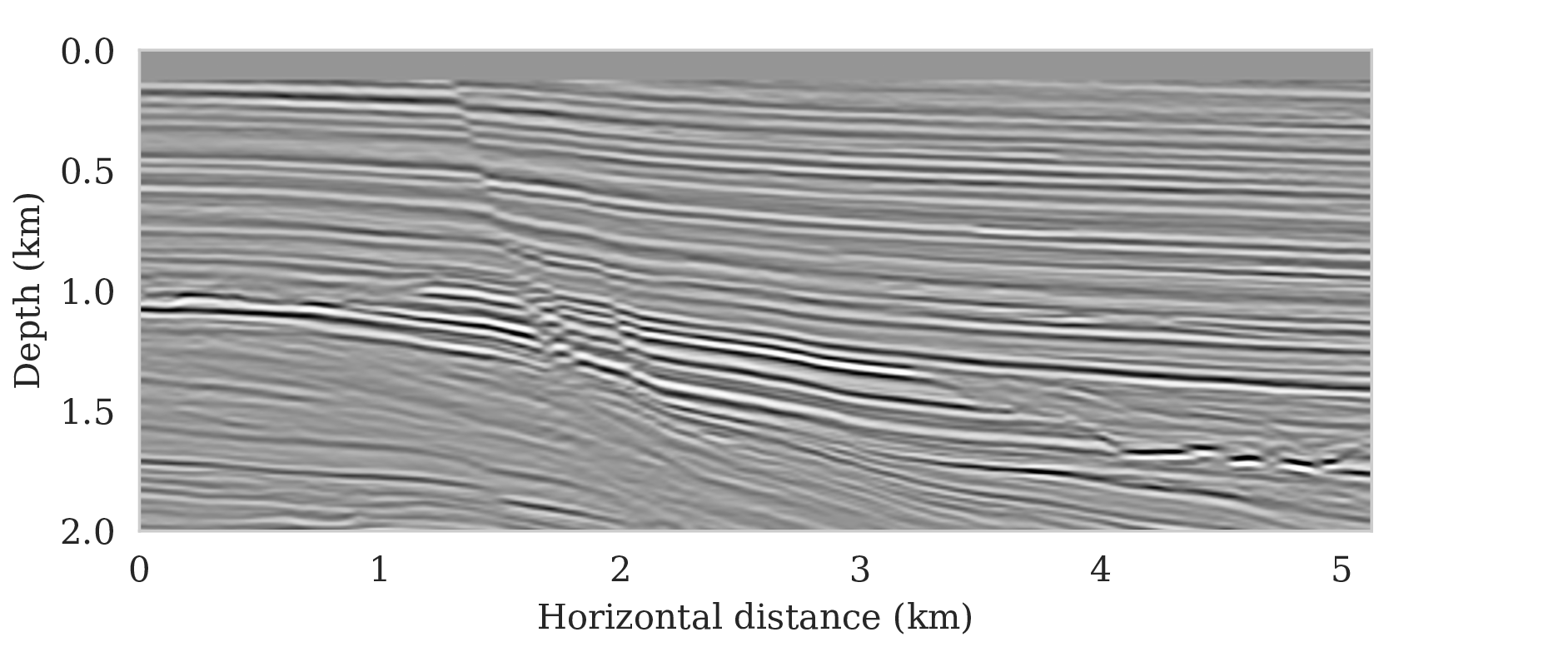
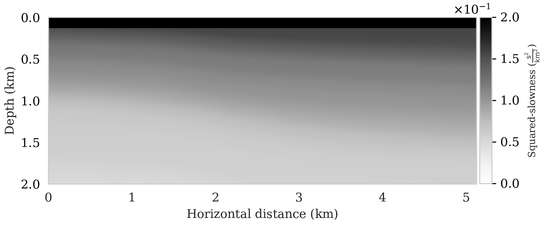
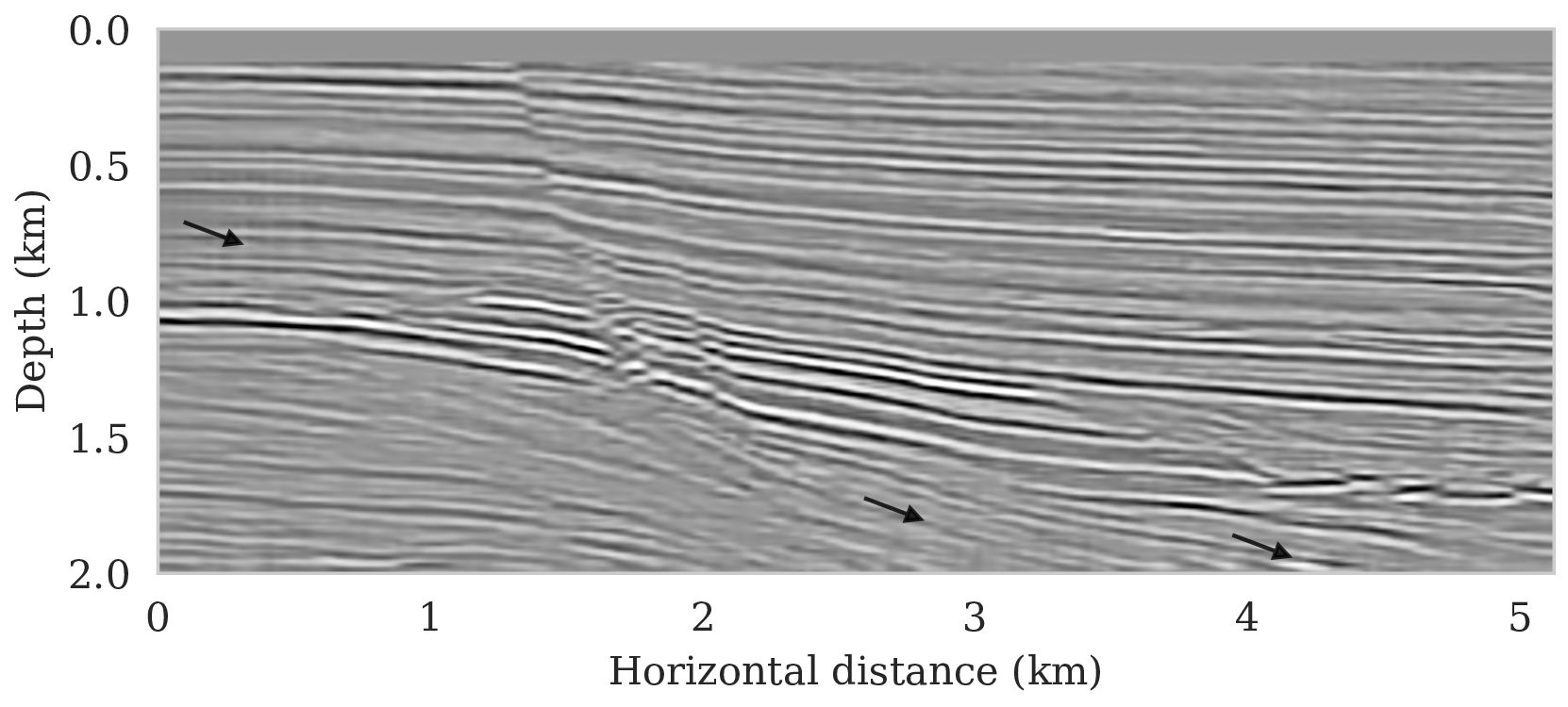
With few exceptions, synthetic models often miss realistic statistics of the spatial distribution of the seismic reflectivity. To avoid working with over simplified seismic images, we generate “quasi”-field shot data derived from a 2D subset of the real prestack Kirchhoff time migrated Parihaka-3D dataset (Veritas, 2005; WesternGeco., 2012) released by the New Zealand government. We call our experiment “quasi” real because synthetic data is generated from migrated field data that serves as a proxy for the unknown true medium perturbations (Figure 1a). Due to the nature of the migration algorithm used to obtain the Parihaka dataset, the amplitudes in the extracted 2D subset are not necessarily consistent with the seismic imaging forward model presented in this paper (equation \(\ref{linear-fwd-op}\)). For this reason, we normalized the amplitudes of the extracted seismic image. Given these perturbations, shot data is generated with the linearized Born scattering operator for a made up, but realistic, smoothly varying background model \(\B{m}_0\) for the squared slowness (Figure 1b). To ensure good coverage, \(205\) shot records are simulated and sampled with a source spacing of \(25\, \mathrm{m}\). Each shot is recorded over \(1.5\) seconds with \(410\) fixed receivers sampled at \(12.5\, \mathrm{m}\) spread across full survey area. The source is a Ricker wavelet with a central frequency of \(30\, \mathrm{Hz}\).

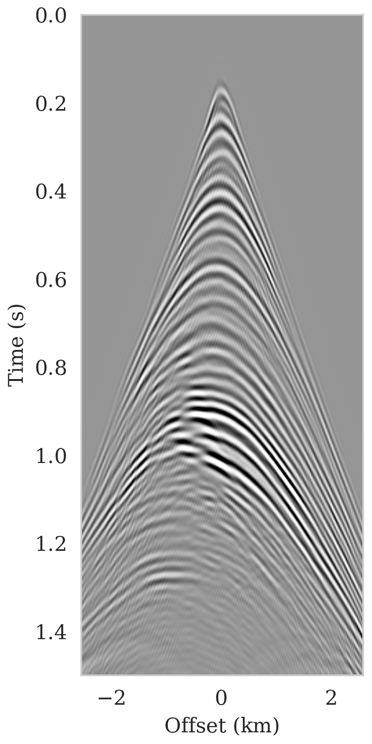
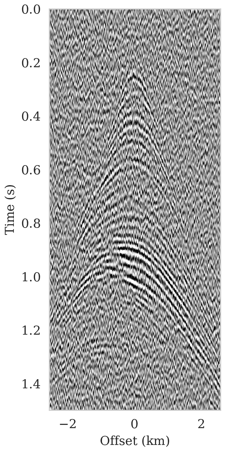
We also add a significant amount of band-limited noise to the shot data by filtering Gaussian white noise with the source wavelet. The resulting signal-to-noise ratio for all data is \(-8.74\, \mathrm{dB}\), which is low. Figure 2 shows an example of a single noise-free (Figure 2a) and noisy (Figure 2b) shot record.

Even though our example is in 2D, the number of parameters (the weights of the deep prior network) is large (approximately \(40\) times larger than image dimension), which results in many SGLD iterations. In a setting where we are content with approximate Bayesian inference, i.e., where the validity of the Markov chains can be established qualitatively in the way described earlier, we found that ten thousand iterations are adequate. We adopt the general practice of discarding the first half the MCMC iterations (about \(25\) passes over the data) (Gelman et al., 2013), which leaves five thousand iterations dedicated to posterior sampling phase (D. Zhu and Gibson, 2018). The stepsize sequence is chosen according to equation \(\ref{stepsize}\) with \(a,\ b\) chosen such the stepsize decreases from \(10^{-2}\) to \(5 \times 10^{-3}\).

Imaging with versus without the deep prior

For reference, we first compare imaging results with and without regularization. The latter is based on maximizing the likelihood (equation \(\ref{MLE}\)) whereas the former involves maximizing the posterior distribution (equation \(\ref{MAP-w}\)). To prevent overfitting of the MLE estimate, the number of iterations is limited to the equivalent of only four data passes (four loops over all shots). To ensure convergence, the number of data passes (or epochs) for the MAP estimate was set to \(15\) (about three thousand iterations). Since the ground truth is known, the optimal value for the \(\lambda^{-2}=5 \times 10^{-3}\) was found by grid search and picking the value that visually limits imaging artifacts. Results of minimizing the negative log-likelihood and negative log-posterior are included in Figures 3a and 3b, respectively. We obtained these results with the RMSprop optimization algorithm (Tieleman and Hinton, 2012), which uses the same preconditioning scheme (equations \(\ref{ruunning-grad}\) and \(\ref{precond-mat}\)) as SGLD that we will use later to conduct Bayesian inference. Compared to vanilla SGD with a fixed stepsize, RMSprop is an adaptive stepsize method conducive to the preconditioner introduced in equations \(\ref{ruunning-grad}\) and \(\ref{precond-mat}\). As with the SGLD updates, the gradient calculations involve a single randomly selected shot record. As expected, compared to the MAP estimate with signal-to-noise ratio (SNR) \(8.79\,\)dB, the MLE estimate (SNR \(8.25\,\)dB) lacks important details, e.g., weak reflectors in deeper sections, and exhibits strong artifacts, including imaged reflectors that are noisy and lack continuity. The latter is important since the estimated seismic image will be used to automatically track horizons.

Bayesian inference with deep priors

As the comparison between MLE and MAP estimates clearly showed, regularization improves the image but important issues remain. First, the use of deep priors can lead to overfitting even when a Gaussian prior on the weights is included. As reported in the literature (Lempitsky et al., 2018; Cheng et al., 2019), stopping early can be a remedy but a stopping criterion remains elusive rendering this type of regularization less effective. Second, the uncertainty is not captured by the MAP estimation. As we will demonstrate, the ability to draw samples from the posterior remedies these issues.

Conditional mean

As described earlier, samples from the posterior provide access to useful statistical information including approximations to moments of the distribution such as the mean. With the minor modifications proposed by Chunyuan Li et al. (2016) to the RMSprop optimization algorithm, the posterior distribution can be sampled with Algorithm 1 after a warmup phase of about \(25\) data passes. The resulting samples for the weights are then used, after push forward (see equation \(\ref{push-forward}\)), to approximate the conditional mean, \(\delta \B{m}_{\text{CM}}\), by computing the sum in equation \(\ref{conditionalmean}\). Compared to the MAP estimate (Figures 3b and 3c), the \(\delta \B{m}_{\text{CM}}\) (SNR \(9.66\,\)dB) is tantamount to another significant improvement especially for weaker reflectors in the deeper part of the image and for reflectors denoted by the arrows.

While there has been a debate in the literature on the accuracy of the MAP versus conditional mean estimates in the context of regularization with handcrafted priors, such as total variation (Burger and Lucka, 2014), we find that the conditional mean estimate negates the need to stop early and is also more robust with respect to noise.

Pointwise standard deviation and histograms

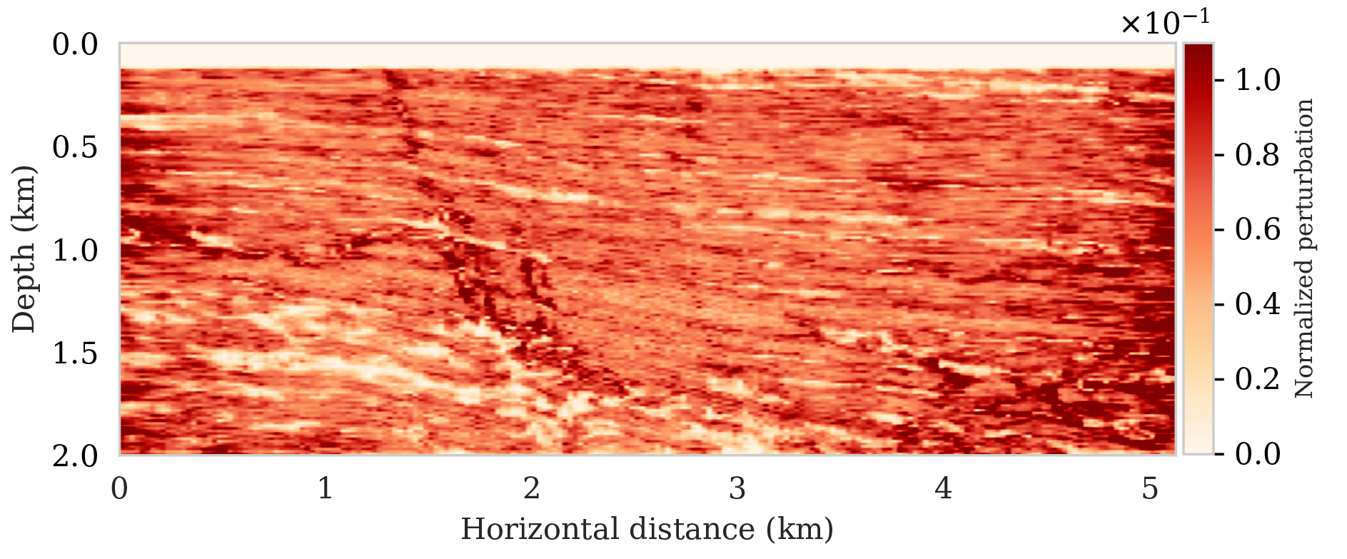
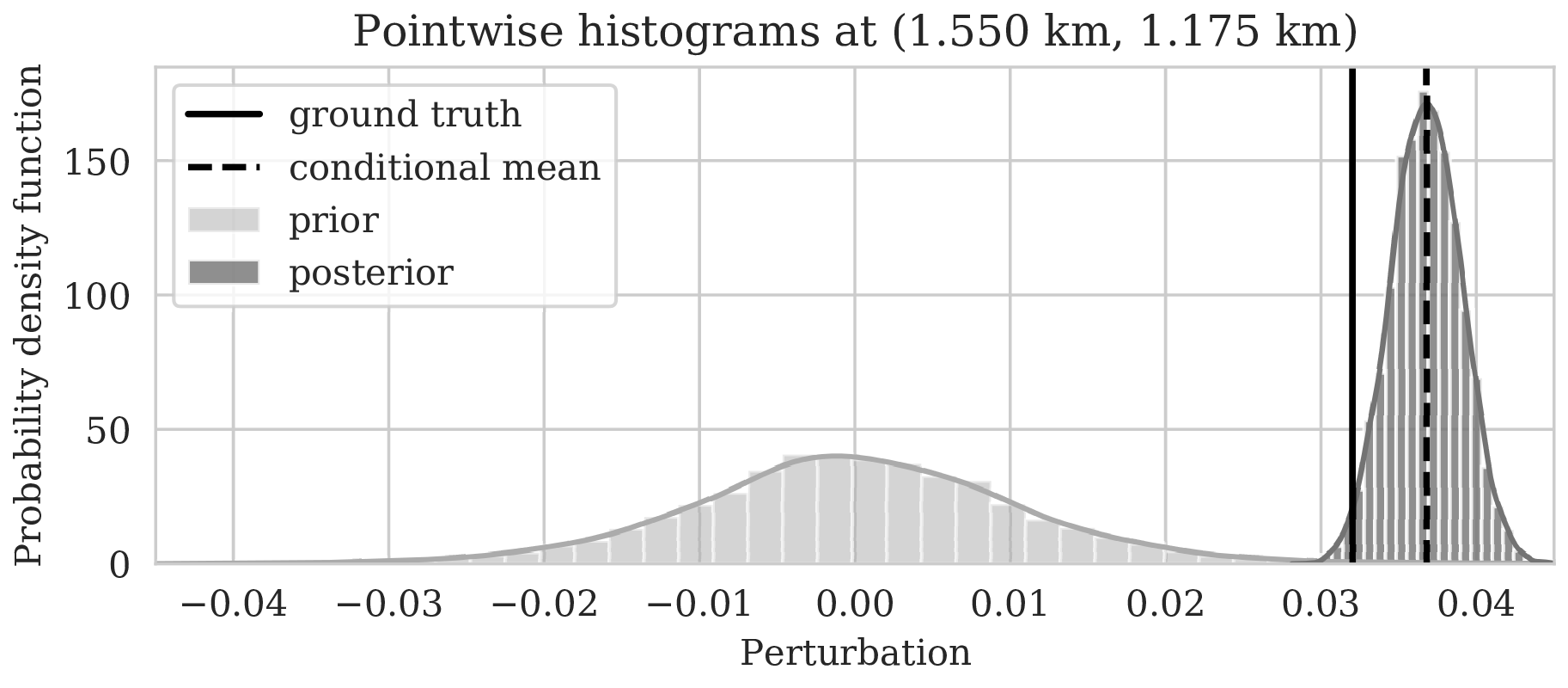
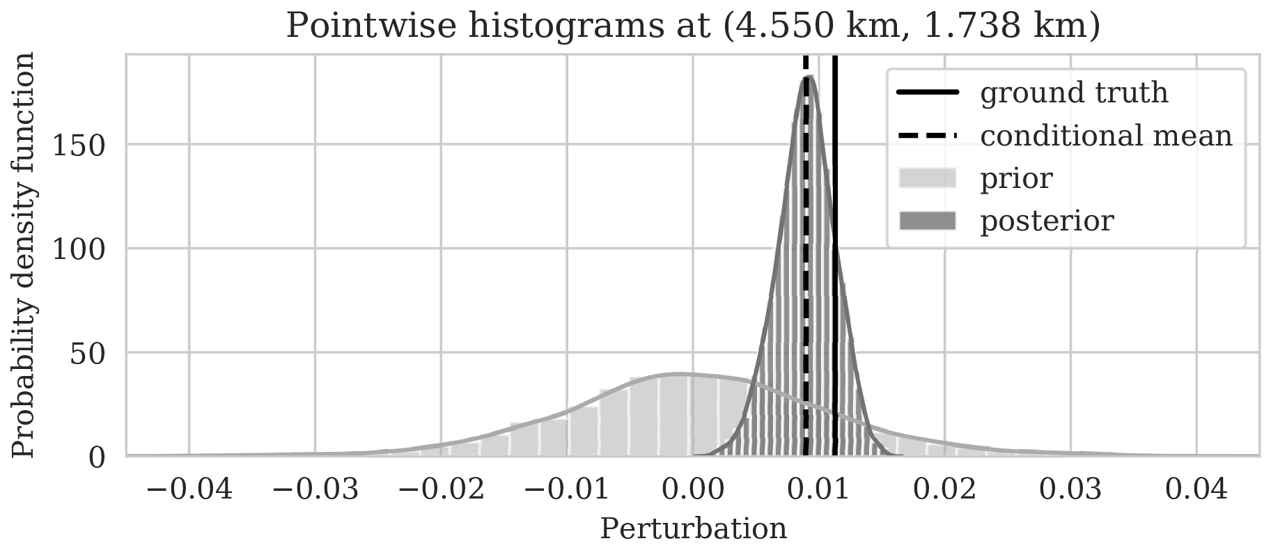
To assess variability among the different samples from the posterior, we include a plot of the pointwise standard deviation \(\boldsymbol{\sigma}_{\text{post}}\) (equation \(\ref{pointwise-std}\)) in Figure 4a. This quantity is a measure for uncertainty. To avoid bias by strong amplitudes in the estimated image, we also plot the stabilized division of the standard deviation by the envelope of the conditional mean in Figure 4b. From these plots in Figure 4, we observe that as expected uncertainty is large in areas with a complex geology, e.g., along the faults and along the tortuous reflectors, and in areas with relative poor illumination deep in the image and near the edges. On the other hand, the shallow areas of the image exhibit low uncertainty, which is to be expected due to proximity to the sources and receivers.

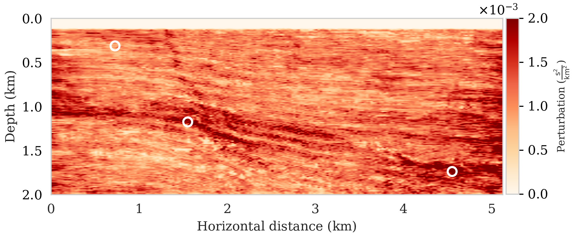
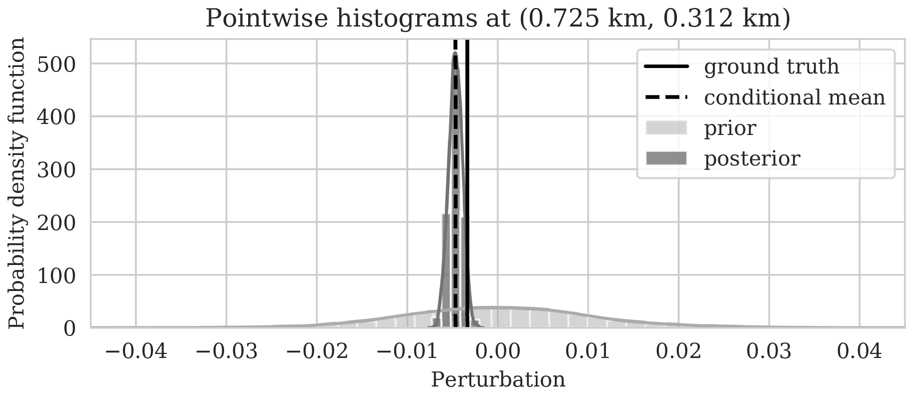
To illustrate how the posterior regularized by the deep prior is informed by the likelihood, we also calculated histograms at three locations denoted by the white circles in Figure 4a. Histograms from the prior are calculated by randomly sampling network weights from the prior distribution, i.e., \(\mathrm{N}(\B{w} \mid \B{0}, \lambda^{-2}\B{I})\), followed by computing the deep prior network’s output for a random but fixed \(\B{z}\). The resulting histograms are plotted in light gray in Figure 5. Similarly, histograms for the posterior are computed (equation \(\ref{push-forward}\)) from samples of the posterior for the weights. These are plotted in dark gray. As expected, the histograms for the posterior are considerably narrower than those of the prior, which means that the posterior is informed by the shot data. We also see that the width of the histograms increases in areas with larger variability. For comparison, we added the conditional mean estimates with dashed vertical line. When compared with the ground truth values denoted by the solid vertical lines, we observe that the ground truth falls inside of the nonzero pointwise posterior interval, which confirms the benefits of the prior.

Accuracy and convergence verification

Drawing samples from the posterior distribution via Markov chains can be subject to errors when the chain is not long enough (Gelman et al., 2013). Unfortunately, the required length of the chain is often infeasible in practice, certainly when the forward operators is expensive to calculate as is the case with our imaging examples. As explained earlier, we qualitative verify the accuracy of the Bayesian inversion by comparing MAP estimates with confidence intervals (Hastie et al., 2001) and by running different Markov chains (Z. Fang et al., 2018).

Consistency with empirical confidence intervals

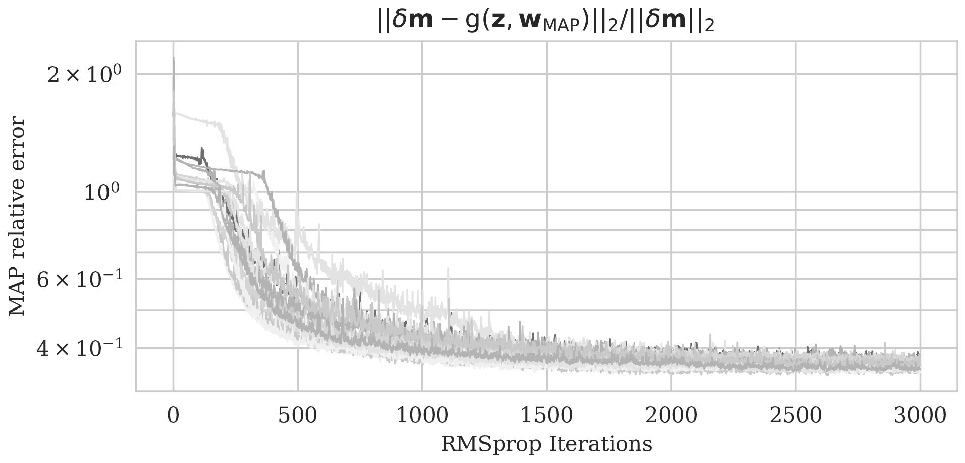
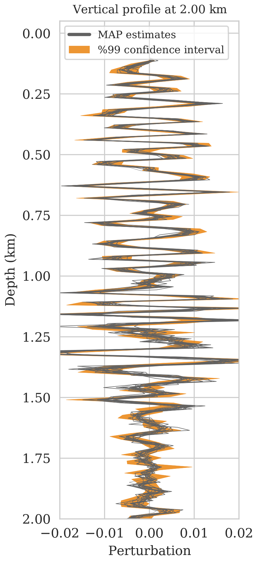
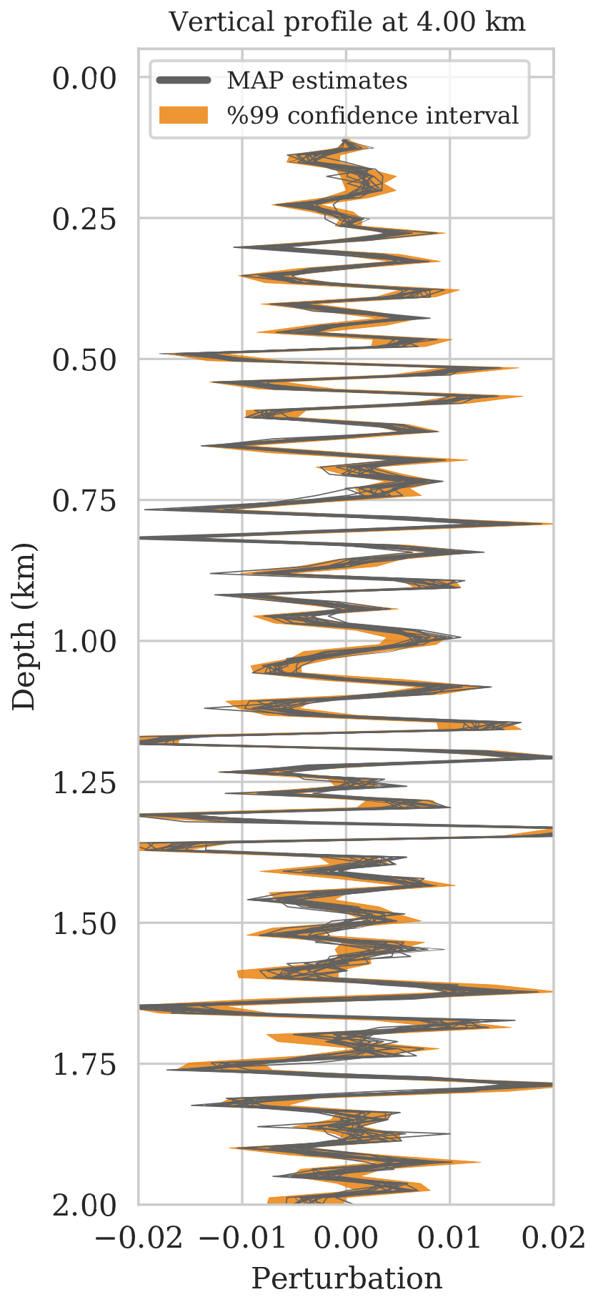
As a first assessment of the accuracy of the MCMC sampling, we computed the relative errors of \(15\) MAP estimates with respect to the ground truth image obtained for a single fixed \(\B{z}\) but different initializations of the network weights. The decay of the relative \(\ell_2\)-norm error for each run over \(3\mathrm{k}\) iterations are plotted in Figure 6a and show relatively small variations from random realization to random realization. Vertical profiles of the MAP estimates at two lateral positions confirm this behavior. With few exceptions, these different MAP estimates fall well within the shaded \(99\%\) confidence intervals plotted in Figures 6b and 6c. The confidence intervals themselves were derived from samples of the posterior. Except for perhaps the deeper part of the model, we can be confident that the Bayesian inference is reasonable certainly in the light of the nonlinearity of the deep prior itself.

Chain to chain variations

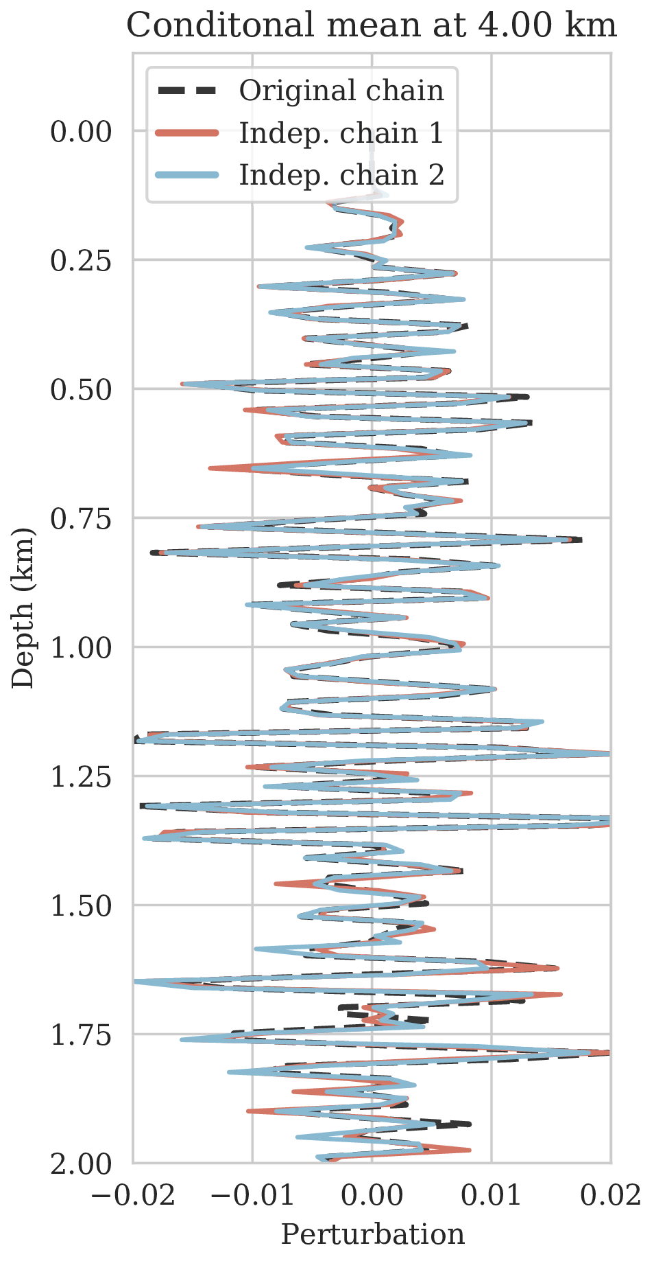
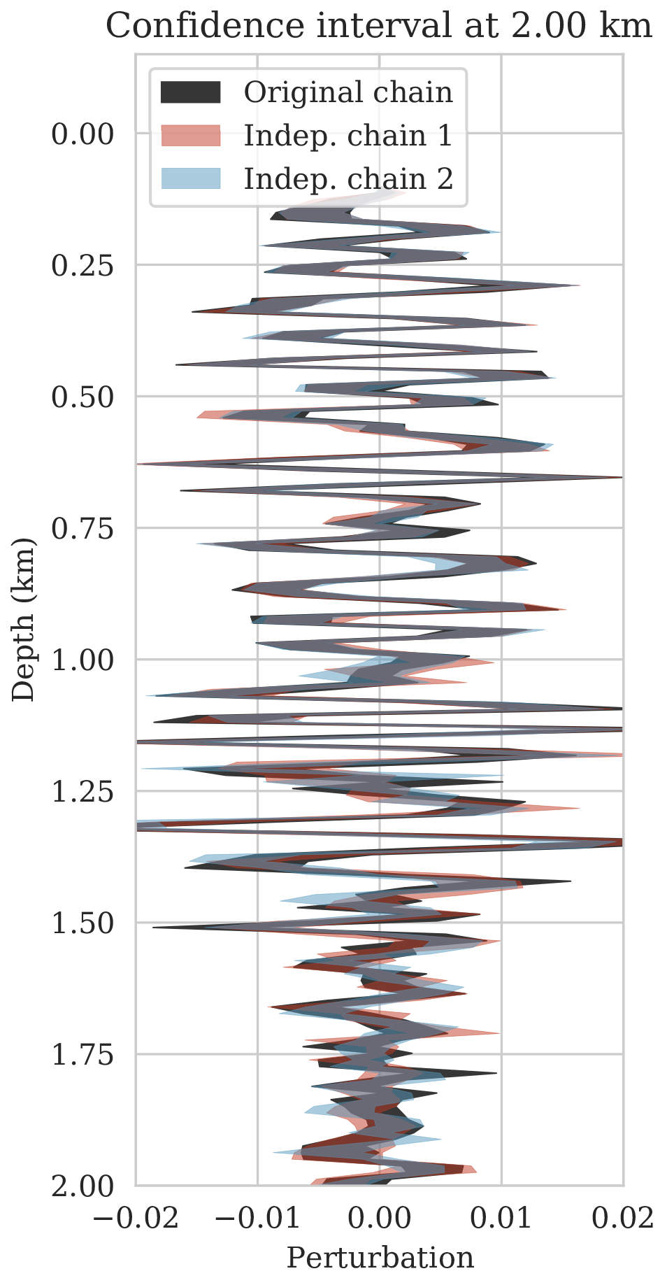
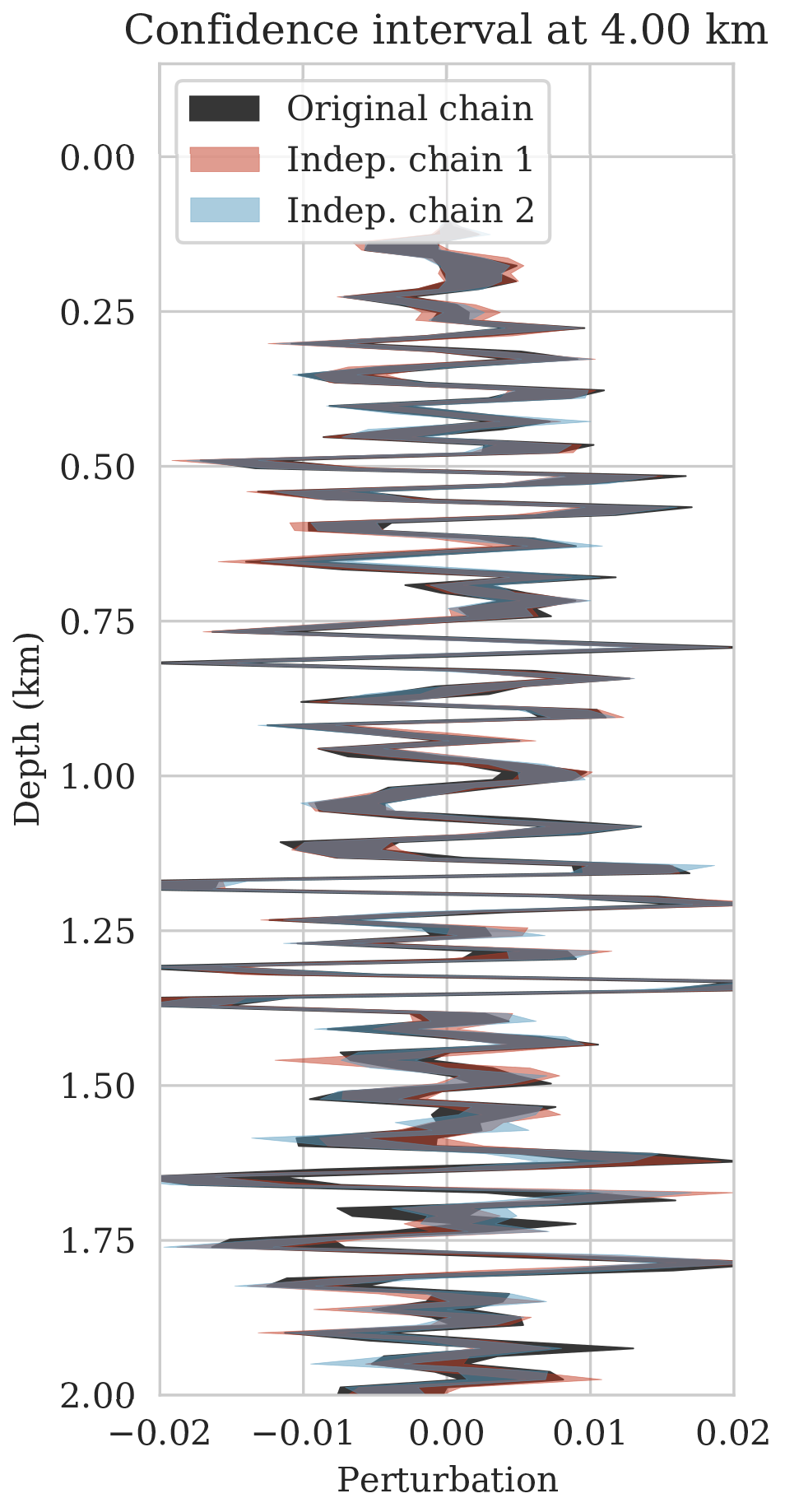
To further assure our Bayesian inference is accurate, we conducted a second experiment comparing estimates for the conditional mean and confidence intervals for three different Markov chains computed from independent random initialization for the weights and \(\B{z}\) fixed. Since we can not afford to run the Markov chains to convergence, we expect slightly different results for the conditional mean and confidence intervals. As observed from Figure 7, this is indeed the case but the variations are relatively minor and confined to the deeper part of the image. This qualitative observation, in conjunction with the behavior of the MAP estimates, suggests that we can be confident that the presented Bayesian inference is reasonably accurate certainly given the task of horizon tracking at hand.

Probabilistic horizon tracking

Typically, seismic images serve as input to a decision process involving identification of certain attributes within the image preferably including an assessment of their uncertainty. With very few exceptions (G. Ely et al., 2018), these assessments of risk are not based on a systematic approach where errors in shot data are propagated to uncertainty in the image and subsequent tasks. To illustrate how the proposed Bayesian inference can serve to assess uncertainty on downstream tasks, we consider horizon tracking, where reflector horizons are extracted automatically from seismic images given a limited number of user specified control points. Typically, these control points are either derived from well data available in the area or from human interpretation. The horizon tracking can be deterministic, i.e., horizons are determined uniquely given a seismic image, or more realistically, it may be nondeterministic, i.e., multiple possible horizons explaining a single image. In either case, the task of delineating the stratigraphy automatically with no to little intervention by interpreters is challenging certainly in areas where the geology is complex, e.g., near faults. To resolve these complex areas high quality images including information on uncertainty are essential.

To set the stage to put tasks conducted on seismic images on a firm statistical footing, we will make the assumption that these tasks are only informed by the estimated image and not by the shot data explicitly. This means when given an estimated image the task, e.g., of horizon tracking, is assumed to be statistically independent of the shot data. Formally, this conditional independence can be expressed as \[ \begin{equation} ( \B{h} \mathrel{\text{$\perp\mkern-10mu \perp$}} \B{d}) \mid \delta \B{m}, \label{conditional-independence} \end{equation} \] where the random variable \(\B{h}\) encodes tracked horizons. The symbol \(\mathrel{\text{$\perp\mkern-10mu \perp$}}\) represents conditional independence (Dawid, 1979) in this case between the estimated horizons and shot records, given the seismic image, i.e., the seismic images, \(\delta \B{m}\), obtained from the shot records, \(\B{d}\), contain all the needed information to predict horizons, \(\B{h}\). The assumed statistical independence implies that the tracked horizons, \(\B{h}\), can be predicted unequivocally from estimated images. Because of the independence, shot data does not bring forth additional information on the horizons. For the remainder of this paper, we denote the task on the image by \(\mathcal{H}\), which for horizon tracking implies \(\B{h}=\mathcal{H}(\delta\B{m})\).

Bayesian formulation

Given the mapping from image to horizons, let \(p_{\mathcal{H}} \left (\B{h} \mid \delta \B{m} \right )\) represent the conditional PDF of horizons given an estimate for the seismic image. This distribution is characterized by the nondeterministic behavior of \(\mathcal{H}\) and assigns probabilities to horizons in the image, \(\delta \B{m}\). In the case where \(\mathcal{H}\) represents automatic horizon tracking this mapping requires control points as an additional input. In this context, sampling from the conditional distribution is equivalent to performing automatic horizon tracking with different realizations of the control points. Alternatively, when \(\mathcal{H}\) represents actions by human interpreters, samples from \(p_{\mathcal{H}} \left (\B{h} \mid \delta \B{m} \right )\) can be thought of as horizons tracked by different individuals.

Provided samples from \(p_{\mathcal{H}} \left (\B{h} \mid \delta \B{m} \right )\) and assuming conditional independence between \(\B{h}\) and \(\B{d}\) given the seismic image described in equation \(\ref{conditional-independence}\), we can perform Bayesian inference with the posterior distribution of horizons, denoted by \(p_{\text{post}} \left (\B{h} \mid \B{d} \right )\). Generally speaking, for any arbitrary function of horizons, \(f\), expectations with respect to \(p_{\text{post}} \left (\B{h} \mid \B{d} \right )\) can be computed as follows: \[ \begin{equation} \begin{aligned} \mathbb{E}_{\B{h} \sim p_{\text{post}} \left (\B{h} \mid \B{d} \right )} \ \left [ f \left (\B{h} \right) \right ] & = \int f \left ( \B{h} \right) p_{\text{post}} \left (\B{h} \mid \B{d} \right ) \mathrm{d} \B{h} = \iint f \left (\B{h} \right) p \left (\B{h}, \delta \B{m} \mid \B{d} \right ) \mathrm{d} \B{h}\, \mathrm{d} \delta \B{m} \\ & = \iint f \left (\B{h} \right) p_{\mathcal{H}} \left (\B{h} \mid \delta \B{m}, \B{d} \right ) p_{\text{post}} \left ( \delta \B{m} \mid \B{d} \right ) \mathrm{d} \B{h}\, \mathrm{d} \delta \B{m} \\ & = \iint f \left (\B{h} \right) p_{\mathcal{H}} \left (\B{h} \mid \delta \B{m} \right ) p_{\text{post}} \left ( \delta \B{m} \mid \B{d} \right ) \mathrm{d} \B{h}\, \mathrm{d} \delta \B{m} \\ & = \mathbb{E}_{\delta \B{m} \sim p_{\text{post}} \left (\delta \B{m} \mid \B{d} \right ) } \left [ \int f \left (\B{h} \right) p_{\mathcal{H}} \left (\B{h} \mid \delta \B{m} \right ) \mathrm{d} \B{h} \right ] \\ & = \underbrace {\mathbb{E}_{\delta \B{m} \sim p_{\text{post}} \left (\delta \B{m} \mid \B{d} \right ) } \underbrace {\mathbb{E}_{ \B{h} \sim p_{\mathcal{H}} \left (\B{h} \mid \delta \B{m} \right ) } \left [ f \left (\B{h} \right) \right ]. }_{\substack{ \text{ uncertainty in} \\ \text{ horizon tracking}}}}_{ \substack{\text{ uncertainty in} \text{ seismic imaging}}} \\ \end{aligned} \label{horizon-inference} \end{equation} \] The second equality in the first line of equation \(\ref{horizon-inference}\) follows from the law of total probability², the second line is obtained by applying the chain rule of PDFs³ to the joint density \(p \left (\B{h}, \delta \B{m} \mid \B{d} \right )\), and the third line exploits the conditional independence assumption in equation \(\ref{conditional-independence}\). Conceptually, equation \(\ref{horizon-inference}\) states that we can decompose the uncertainty in horizon tracking into two parts, namely uncertainty in imaging and uncertainty in the horizon tracking task itself. Based on equation \(\ref{horizon-inference}\), expectations over \(p_{\text{post}} \left (\B{h} \mid \B{d} \right )\) can be calculated via Monte Carlo integration using samples from \(p_{\text{post}} \left (\B{h} \mid \B{d} \right )\). Thanks to the conditional independence assumption in equation \(\ref{conditional-independence}\), we can sample from \(p_{\text{post}} \left (\B{h} \mid \B{d} \right )\) by sampling the imaging posterior, \(p_{\text{post}} \left (\delta \B{m} \mid \B{d} \right )\), followed by tracking the horizons in each seismic image. This step yields an ensemble of possible horizons for each sampled image. Using samples drawn from \(p_{\text{post}} \left (\B{h} \mid \B{d} \right )\), we approximate the expectation in equation \(\ref{horizon-inference}\) by the sample mean. In the following sections, we break equation \(\ref{horizon-inference}\) down into two cases where the horizon tracker yields an unique set of horizons or multiple sets of likely horizons, given one seismic image.

Case \(1\): horizons are unique given an image

In the simplest case, where horizon tracking uniquely determines the horizons given a seismic image, the conditional PDF \(p_{\mathcal{H}} \left (\B{h} \mid \delta \B{m} \right )\) corresponds to a delta function, i.e., we have \[ \begin{equation} \begin{split} p_{\mathcal{H}}(\B{h} \mid \delta \B{m}) = \delta_{\left [ \B{h} = \mathcal{H} \left ( \delta \B{m} \right ) \right ]} \left (\B{h} \right ), \\ \end{split} \label{probH} \end{equation} \] where \(\mathcal{H}\) represent the deterministic horizon tracking map and \(\delta(\cdot)\) stands for the delta Dirac distribution. Substituting equation \(\ref{probH}\) into equation \(\ref{horizon-inference}\) yields \[ \begin{equation} \begin{aligned} \mathbb{E}_{\B{h} \sim p_{\text{post}} \left (\B{h} \mid \B{d} \right )} \ \left [ f \left (\B{h} \right) \right ] & = \mathbb{E}_{\delta \B{m} \sim p_{\text{post}} \left (\delta \B{m} \mid \B{d} \right ) } \left [ \int f \left (\B{h} \right) \delta_{\left [\B{h} = \mathcal{H} \left ( \delta \B{m} \right ) \right ]} \left (\B{h} \right ) \mathrm{d} \B{h} \right ], \\ & = \mathbb{E}_{\delta \B{m} \sim p_{\text{post}} \left (\delta \B{m} \mid \B{d} \right ) } \left [ f \left ( \mathcal{H} \left ( \delta \B{m} \right ) \right ) \right ], \\ & \approx \frac{1}{n_{\mathrm{w}}}\sum_{j=1}^{n_{\mathrm{w}}} f \left ( \mathcal{H} ( {\delta \B{m}}_j ) \right ), \\ \end{aligned} \label{independence-det} \end{equation} \] where \(\left \{ {\delta \B{m}}_j \right \}_{j=1}^{n_{\mathrm{w}}} \sim p_{\text{post}} ( \delta \B{m} \mid \B{d} )\) are \(n_{\mathrm{w}}\) samples from the posterior distribution. Equation \(\ref{independence-det}\) essentially means that in case of a deterministic horizon tracker uncertainty in imaging can be translated to uncertainty in horizon tracking by simply drawing samples from the seismic imaging posterior and tracking horizons in each image. This procedure results in samples from the posterior distribution of horizons and inference of this posterior distribution is done via the equation above.

Case \(2\): multiple likely horizons given an image

The probabilistic horizon tracking approach, described in equation \(\ref{horizon-inference}\), also admits nondeterministic horizon trackers, e.g., automatic horizon tracking with uncertain control points, e.g., points provided by multiple human interpreters. In this case, instead of having one set of horizons for each seismic image, we have multiple realizations of horizons that each agree with a seismic image, i.e., they are samples from \(p_{\mathcal{H}}(\B{h} \mid \delta \B{m})\). With these samples, the inner expectation in equation \(\ref{horizon-inference}\) can be estimated. Assuming that for each image we have \(n_h\) different realizations of tracked horizons, namely, \(h_k^{(\delta \B{m})} \sim p_{\mathcal{H}}(\B{h} \mid \delta \B{m}), \ k=1,\cdots, n_h\), equation \(\ref{horizon-inference}\) becomes \[ \begin{equation} \begin{aligned} \mathbb{E}_{\B{h} \sim p_{\text{post}} \left (\B{h} \mid \B{d} \right )} \ \left [ f \left (\B{h} \right) \right ] & = \mathbb{E}_{\delta \B{m} \sim p_{\text{post}} \left (\delta \B{m} \mid \B{d} \right ) } \mathbb{E}_{ \B{h} \sim p_{\mathcal{H}} \left (\B{h} \mid \delta \B{m} \right ) } \left [ f \left (\B{h} \right) \right ] \\ & \approx \mathbb{E}_{\delta \B{m} \sim p_{\text{post}} \left (\delta \B{m} \mid \B{d} \right ) } \left [ \frac{1}{n_h} \sum_{k=1}^{n_h} f \left ( h_k^{(\delta \B{m})}\right ) \right ], \\ & \approx \frac{1}{n_h n_{\mathrm{w}}} \sum_{j=1}^{n_{\mathrm{w}}} \sum_{k=1}^{n_h} f \left ( h_k^{({\delta \B{m}}_j)}\right ) \end{aligned} \label{sum-horizons-points} \end{equation} \] where \(h_k^{({\delta \B{m}}_j)}\) is the \(k\)th sample from \(p_{\mathcal{H}}(\B{h} \mid {\delta \B{m}}_j)\) and \({\delta \B{m}}_j\) is the \(j\)th sample from \(p_{\text{post}} \left (\delta \B{m} \mid \B{d} \right)\). Because it has an extra sum over the different realizations of tracked horizons for a fixed image, equation \(\ref{sum-horizons-points}\) differs from equation \(\ref{independence-det}\). In the ensuing sections, we show how equations \(\ref{independence-det}\) and \(\ref{sum-horizons-points}\) can be used to calculate pointwise estimates for the first two moments of the posterior distribution over horizons.

Uncertainty quantification in horizon tracking

It is often beneficial to express uncertainty in the form of confidence intervals. For this purpose, equation \(\ref{independence-det}\) or \(\ref{sum-horizons-points}\) is evaluated first for \(f(\B{h}) =\B{h}\). This yields the conditional mean estimate for the horizons denoted by \[ \begin{equation} \boldsymbol{\mu}_{\B{h}} = \mathbb{E}_{\B{h} \sim p_{\text{post}} \left (\B{h} \mid \B{d} \right )} [ \B{h} ]. \label{cm-horizons} \end{equation} \] Similarly, the pointwise standard deviation of the horizons can be computed by choosing \(f(\B{h}) = (\B{h} - \boldsymbol{\mu}_{\B{h}}) \odot (\B{h} - \boldsymbol{\mu}_{\B{h}})\). This latter point estimate can be calculated via \[ \begin{equation} \boldsymbol{\sigma}^2_{\B{h}} = \mathbb{E}_{\B{h} \sim p_{\text{post}} \left (\B{h} \mid \B{d} \right )} [ (\B{h} - \boldsymbol{\mu}_{\B{h}}) \odot (\B{h} - \boldsymbol{\mu}_{\B{h}}) ], \label{std-horizons} \end{equation} \] where \(\boldsymbol{\sigma}_{\B{h}}\) denotes the pointwise standard deviation. The \(99\%\) confidence interval for horizons is the interval \(\boldsymbol{\mu}_{\B{h}} \pm 2.576\, \boldsymbol{\sigma}_{\B{h}}\). Contrary to most existing automatic horizon trackers, the uncertainty estimates we provide here are determined by uncertainties in the image due to noise, and possibly linearization errors, in the shot records.

Probabilistic horizon tracking—“ideal low-noise” Parihaka example

The main goal of this paper is to derive a systematic approach to propagate uncertainty in imaging to the task at hand. For this purpose, we first consider the relatively ideal case of uncertainty due to additive random noise in the shot data. To illustrate how the presence of this noise affects the task of horizon tracking, we apply the proposed probabilistic framework to the Parihaka imaging example discussed earlier. Because the seismic shot data for this example is relatively low-frequency (\(30\,\)Hz source peak frequency) and the geology relatively simple, horizons are not that challenging to track. However, there is a substantial amount of noise in the shot data that we need to contend with when tracking the imaged horizons. For the latter task, we deploy the tracking approach introduced by Wu and Fomel (2018), which requires the user to provide control points on the seismic horizons of interest.

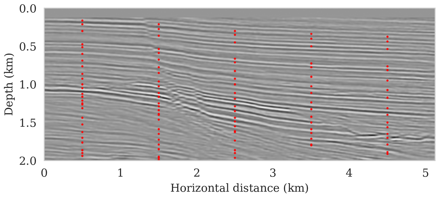
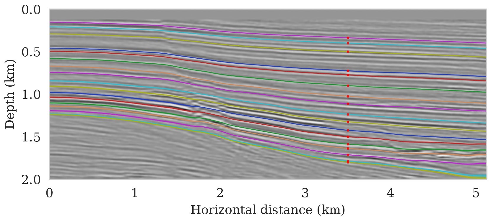
To setup this tasked imaging experiment, we select \(25\) horizons from the conditional mean estimate (Figure 3c) calculated for the Parihaka seismic imaging example. Next, control points are picked for the selected horizons at various horizontal positions, separated by \(1\, \mathrm{km}\). We group the control points with the same horizontal location, yielding five sets of control points. Figure 8 shows these five sets located at lateral positions \(0.5\), \(1.5\), \(2.5\), \(3.5\), and \(4.5\, \mathrm{km}\).

To separate the effect of errors in the shot data and variations amongst provided control points, we consider noisy shot data first, followed by the situation where there is uncertainty due to noise in the shot data and due to variations in the control points.

Uncertainty due to noise in shot data (case 1)

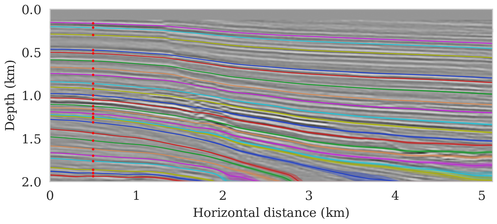
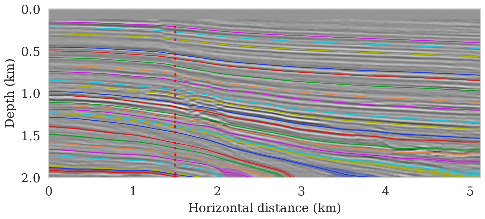
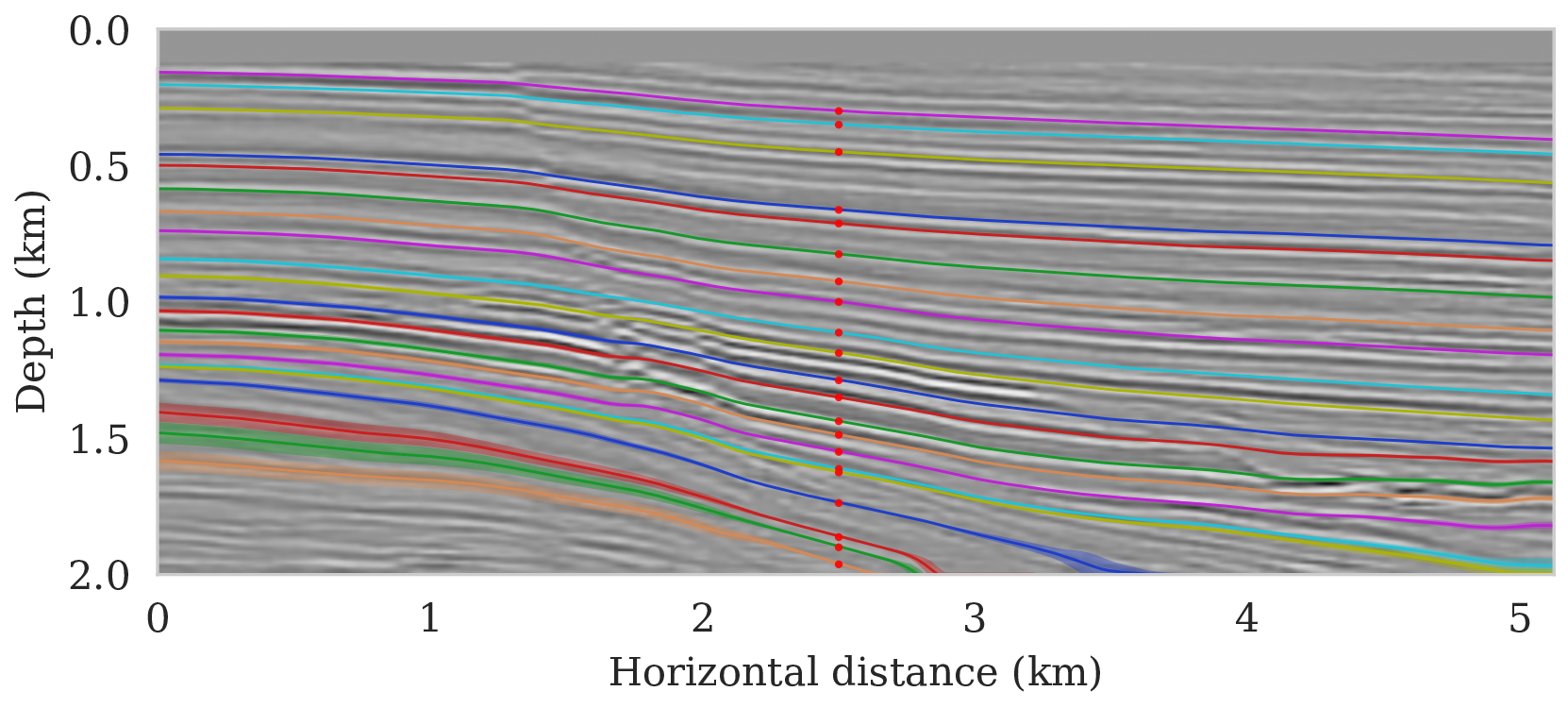
To calculate noise-induced uncertainties in horizon tracking (case 1), we pass samples from the imaging posterior distribution, \(p_{\text{post}} \left (\delta \B{m} \mid \B{d} \right )\), to the automatic horizon tracking software (Wu and Fomel, 2018). Given the five sets of selected control points (Figure 8), the tracker generates for each sample of the imaging posterior \(25\) horizons according to equation \(\ref{independence-det}\). For each set of control points, the conditional mean and \(99\%\) confidence intervals are calculated included in Figure 9. Each plot (Figures 9a – 9e) corresponds to tracked horizons with confidence intervals derived from different sets of control points. As expected, the results exhibit more uncertainty for horizons tracked in the deeper parts of the image and close to boundaries, which is consistent with the relative poor illumination in these areas. Moreover, uncertainty in the tracked locations increases away from the control points. This increase in uncertainty agrees with the inherent challenge of automatic horizon tracking across areas of poor illumination, faults and tortuous reflectors. This behavior is observed for each set of control points.

Aside from shot noise induced uncertainty, variations in the control point may also contribute to uncertainty in the horizon tracking. This corresponds to case 2, which we consider in the next section.

Uncertainty due to noise and uncertain control points (case 2)

The presence of noise in shot data is often not the only cause of uncertainty within the task of (automatic) horizon tracking. Human errors, or better variations in the selection of control points by interpreters, may also contribute to uncertainty. To mimic differences in selected control points, we impose a distribution over the control points. For simplicity, in this example we assume that the five sets of control points are equally likely to be accurate. This is to say, we are equally certain of the accuracy of the picked control points. This can be related to the case where we have access to wells in the seismic survey area and we are certain of the well tying procedure. Other sources of error such as uncertainty in location of the control points, multiple human interpreters, etc, can also be incorporated in the equation \(\ref{sum-horizons-points}\), but will not be considered here. Given the above assumption on the probability distribution, each realization of the seismic image gives rise to multiple equally likely tracked horizons for each of the five sets of control points.

Given these multiple tracked horizons for each image, pointwise first and second moments of \(p_{\mathcal{H}} \left (\B{h} \mid \delta \B{m} \right )\) are calculated via equations \(\ref{cm-horizons}\) and \(\ref{std-horizons}\) by tracking horizons in each sample from the imaging posterior. The horizon tracker yields five sets of horizons for each seismic image, each obtained using one of the five sets of control points. Results of this procedure are summarized in Figure 10. As in the earlier examples, we observe an increase in uncertainty with depth and at the boundaries. Contrary to small uncertainties near the control points, we now observe uncertainty everywhere along the tracked horizons, which suggests increased variability amongst horizons. The variability comes from not trusting only one set of control points, but incorporating information from all the fives sets of control points.

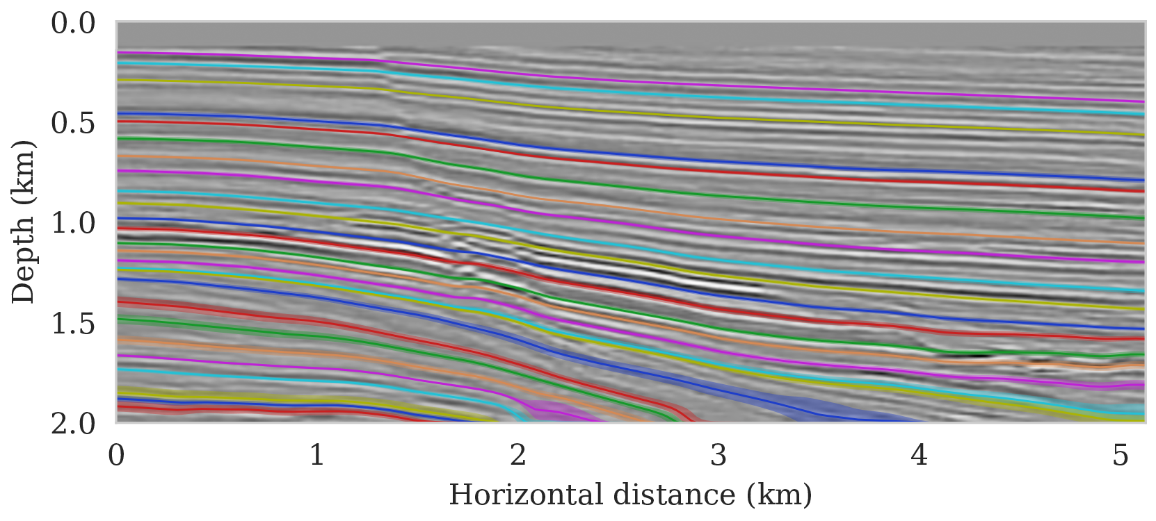
Probabilistic horizon tracking—“noisy” high-resolution Compass model example

While the seismic imaging examples considered so far were directly obtained from migrated shot data of the Parihaka dataset, the linearization errors, i.e., errors due to linearizing the wave equation with respect to the background squared-slowness model, were ignored because the quasi-real data was generated through the demigration process for a made-up background model. Aside from this simplification, the geology of the examples discussed so far was relatively simple and imaged at low resolution. To account for a more realistic setting, involving complex geology and high-resolution imaging, we will quantify imaging and horizon tracking uncertainty given high-frequency but noisy synthetic shot data. To mimic the complexities of field data, noisy shot data—generated with nonlinear forward modeling on a 2D subset of the Compass model (Jones et al., 2012)—is used as input to the proposed imaging scheme. We select the synthetic Compass model because it contains realistic heterogeneity derived from both seismic and well data collected in the North Sea (Jones et al., 2012). Aside from a low signal-to-noise ratio of \(-9.17\, \mathrm{dB}\), this example is affected by linearization errors.

As before, we first describe the problem setup, followed by a comparison between the unregularized MLE and deep-prior regularized MAP and conditional mean estimates. After presenting results on uncertainty quantification on the image, results of our probabilistic horizon tracking framework will be discussed below.

Problem setup

Split spread raw data, consisting of \(101\) shot records sampled with a source spacing of \(25\, \mathrm{m}\) and a receiver sampling \(12.5\, \mathrm{m}\), is generated by solving the acoustic wave equation for the 2D subset of the Compass model. To mimic broadband data, the source is a Ricker wavelet with a central frequency of \(40\, \mathrm{Hz}\). Each shot is \(1.6\) seconds long.

To image the shot data, we first derive a kinematically correct background model via smoothing. Next, linearized data is created by subtracting shot data simulated in this smooth background model from the shot data simulated in the actual model. This data serves as input to our imaging scheme.

Imaging with uncertainty quantification

To arrive at the MLE and MAP estimates for the image, we follow the procedure outlined before. The MLE estimate is obtained by minimizing equation \(\ref{deep-prior-likelihood}\) with stochastic optimization limiting the number of iterations to six passes over the \(101\) shots. Equation \(\ref{deep-prior}\) is minimized with respect to \(\B{w}\) with the RMSprop optimization algorithm (Tieleman and Hinton, 2012) for stepsize of \(10^{-3}\) and five thousand iterations (about \(50\) passes over all shots). We stopped the iterations after no further visual improvement to the image was observed. The value for the tradeoff off parameter, \(\lambda^{-2}=3 \times 10^{-5}\), was set after extensive parameter testing guided by a value that leads to the least amount of visual imaging artifacts.

Compared to the previous example, the MLE image estimate is of poor quality (SNR \(2.80\,\)dB) and contains many imaging artifacts stemming from the noise and linearization errors. The MAP estimate, on the other hand, is improved (SNR \(3.91\,\mathrm{dB}\)) thanks to regularization by the deep prior but it does contain unrealistic artifacts and misses details especially in the deeper parts of the image (juxtapose Figures 11a and 11b). By running Algorithm 1 for ten thousand iterations, we compute five thousand samples from the posterior distribution on the image following the stepsize strategy of equation \(\ref{stepsize}\) with \(\gamma = \frac{1}{3}\) and \(a,\ b\) chosen such the stepsize decreases from \(5 \times 10^{-3}\) to \(10^{-3}\). This took approximately \(18\) hours on a quad-core machine. The resulting estimate for the conditional mean, included in Figure 11c, represents a considerable visual improvement with a SNR of \(4.12\,\)dB. Compared to the MLE and MAP estimates, the conditional mean estimate exhibits more continuous reflectors and significantly fewer artifacts. This example confirms that images yielded by the conditional mean of inverse problems regularized by the deep prior are relatively robust to noise.

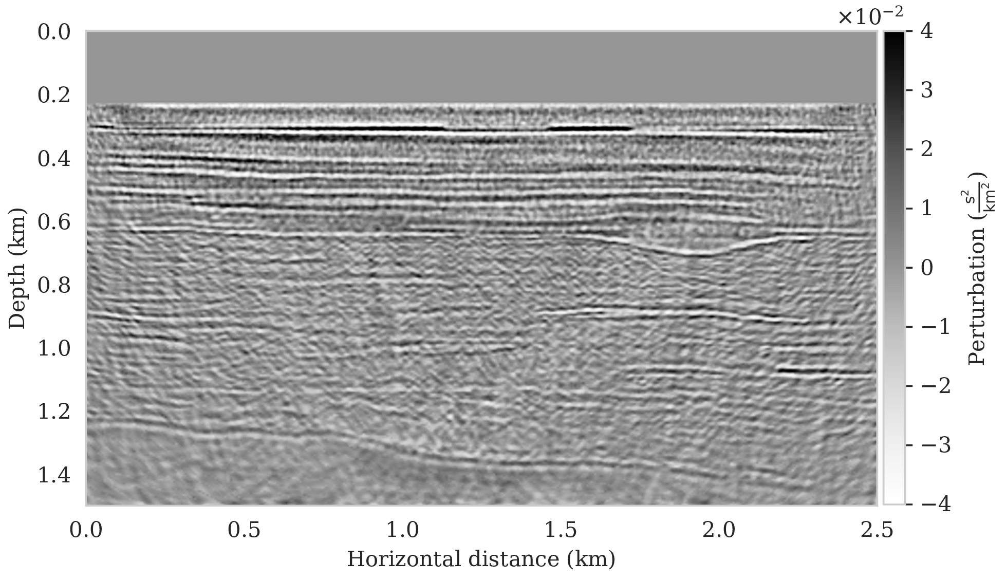
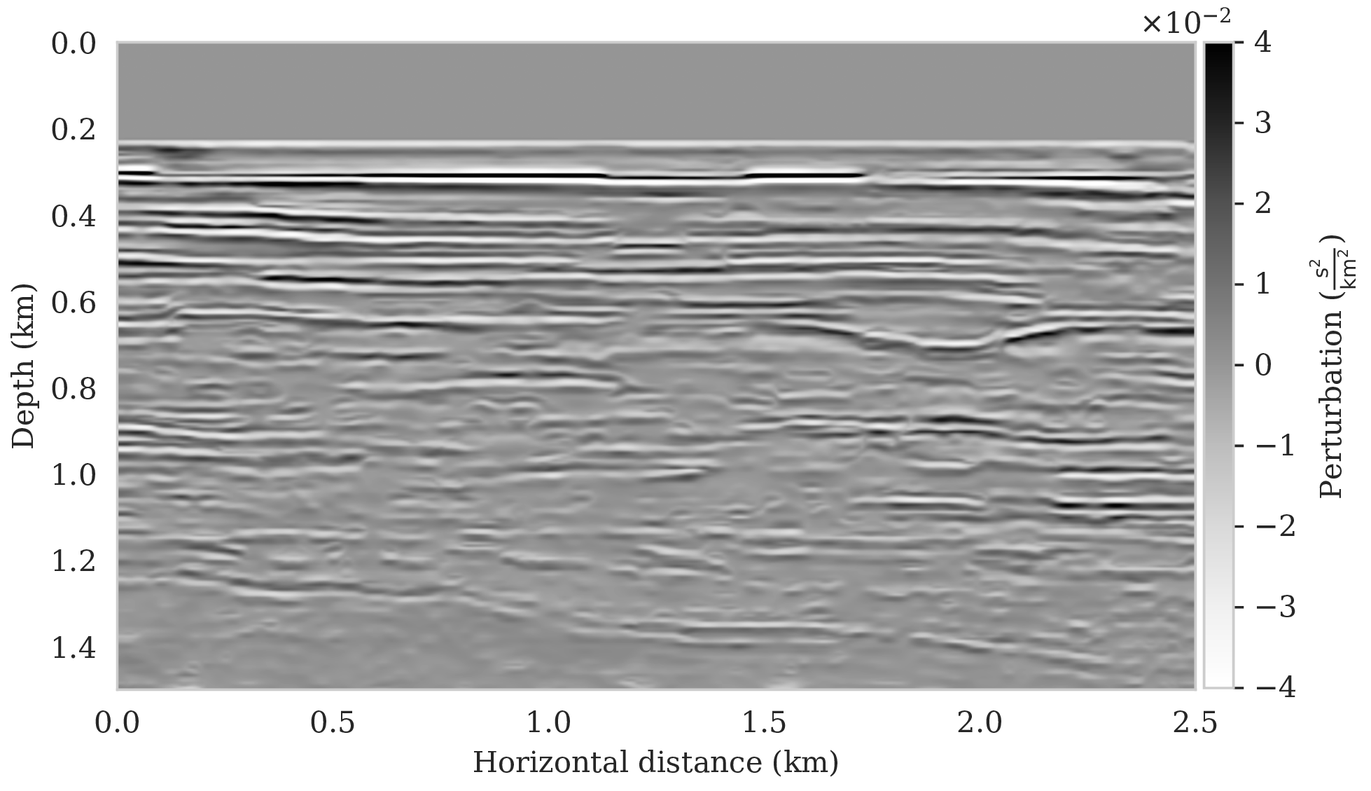
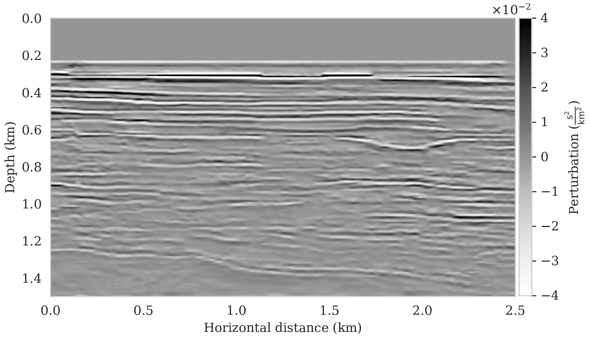
The available samples from the posterior also allows us to calculate an estimate for the pointwise standard deviation of the image. This quantity is plotted in Figure 12a. To avoid overprint by the strong reflectors, we also included a plot of the normalized standard deviation obtained by stabilized division by the conditional mean. Both plots for the pointwise standard deviations show a distinct correlation between difficult to image areas of complex geology, such as channels, and areas affected by relatively poor illumination near the edges and for the deep parts of the image. In the next section, we will show how the samples from the posterior inform the task of horizon tracking.

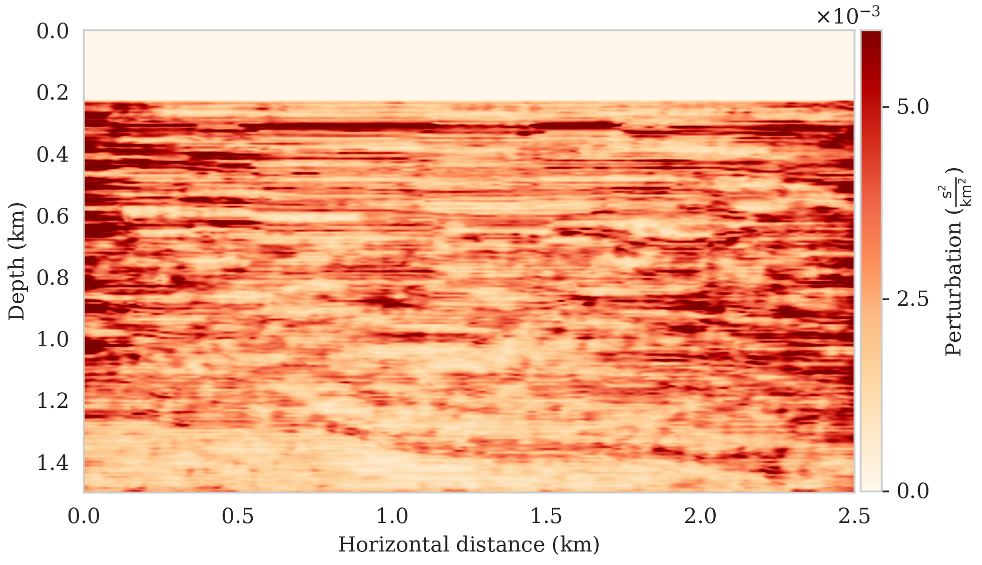
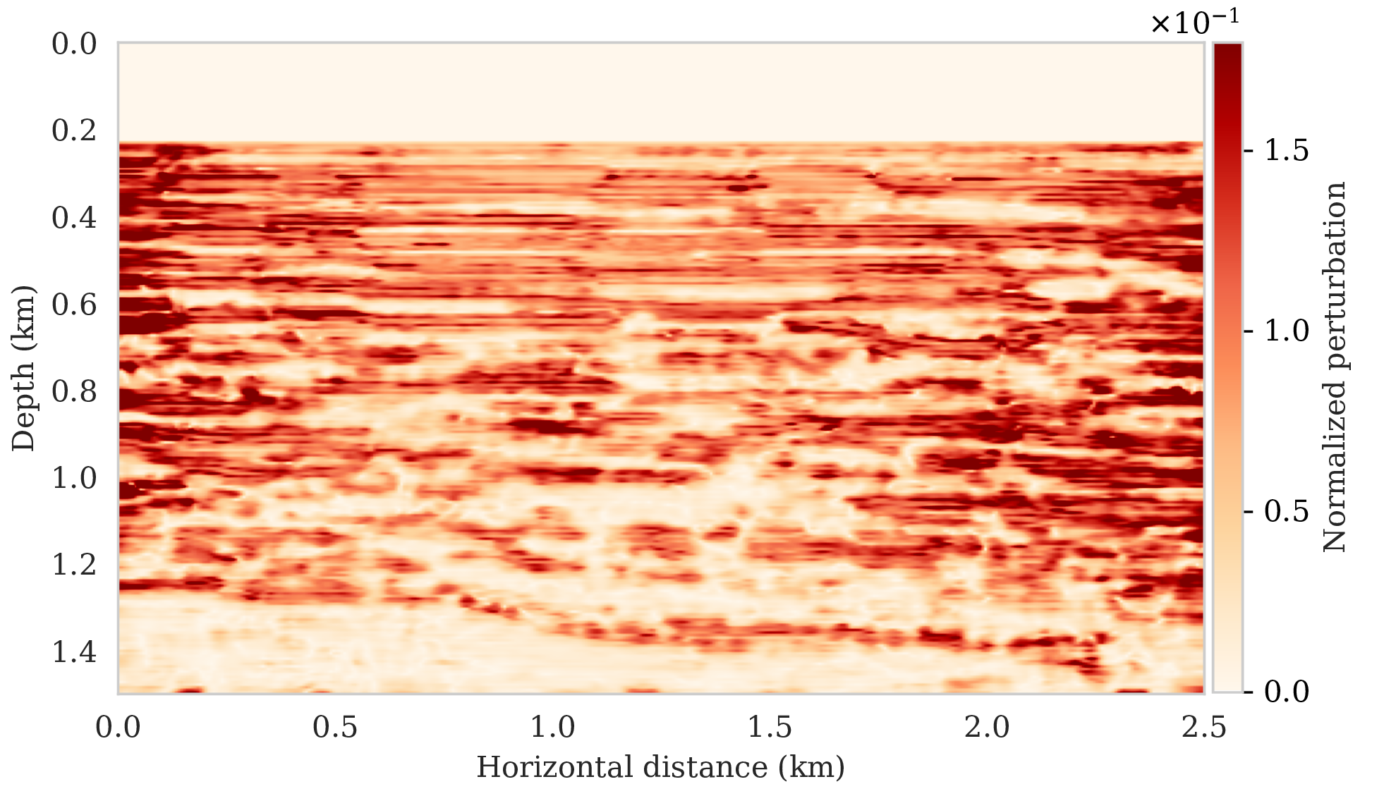
Horizon tracking with uncertainty quantification

Similar to the previous horizon tracking example \(14\) horizons are selected from the conditional mean estimate for the image (Figure 11c). As before, control points are picked for each horizon at the horizontal locations \(62.5\), \(562.5\), \(1062.5\), \(1562.5\), and \(2062.5\, \mathrm{m}\). Control points with the same horizontal position are grouped together, yielding five sets of control points. As before, we distinguish between uncertainties related to noise and now also linearization errors in the data and uncertainty related to errors in the control parameters and in the shot data due to noise and linearization errors.

Uncertainty due to noise and linearization errors in the shot data (case 1)

Tracked horizons plus \(99\%\) confidence intervals for the five sets of control points are included in Figures 13a – 13e. These results were computed by sampling the posterior distribution for horizon tracking, \(p_{\text{post}} \left (\B{h} \mid \B{d} \right)\), following the procedure described above. Not unexpected, we consistently observe increases in uncertainty as we move further away from the control points and deeper into the image. This increase in the size of the confidence interval is due to the increased variability amongst the samples of the imaging posterior especially in regions that are more difficult to image, e.g., near the boundaries of the image, at the deeper parts and near regions of complex geology.

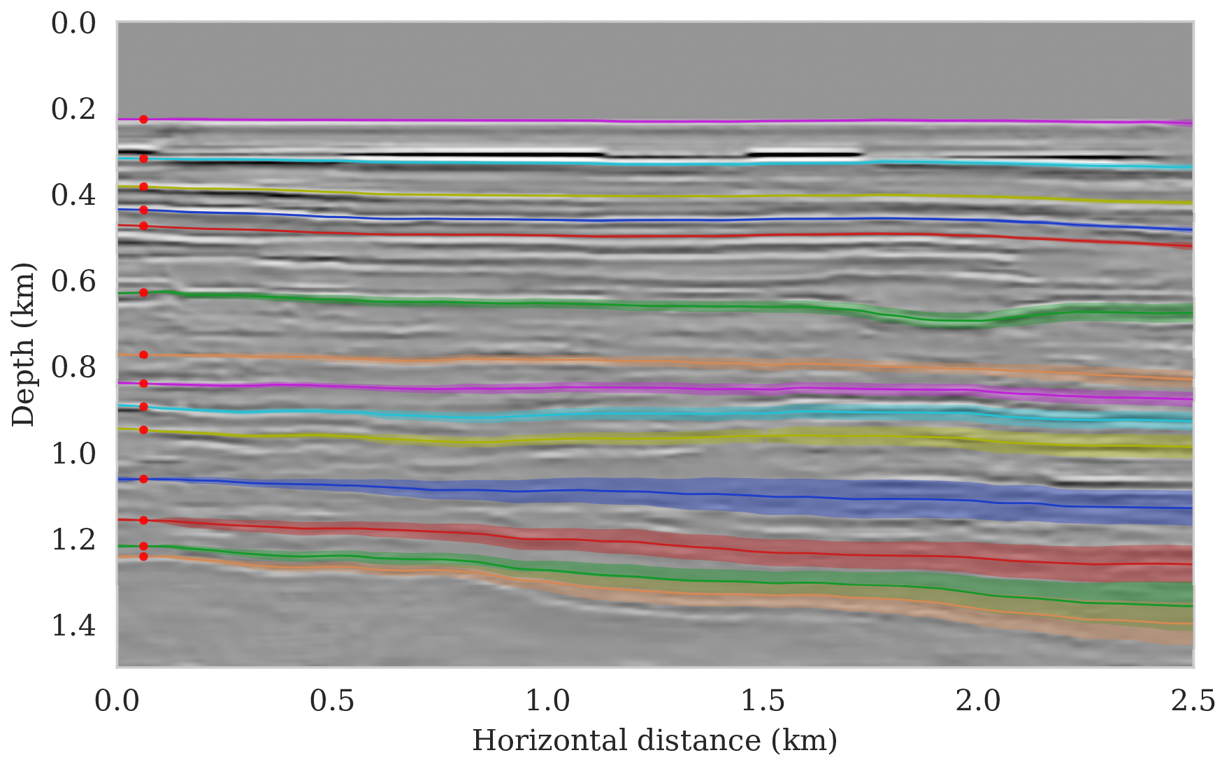
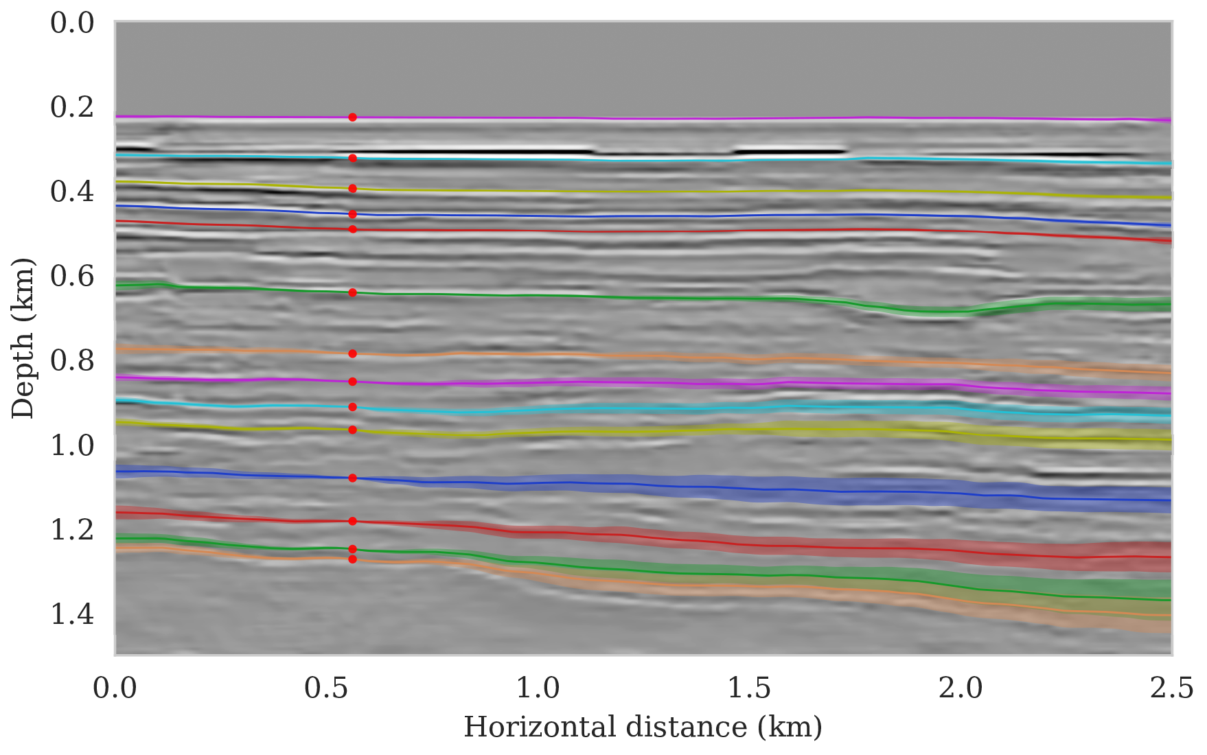
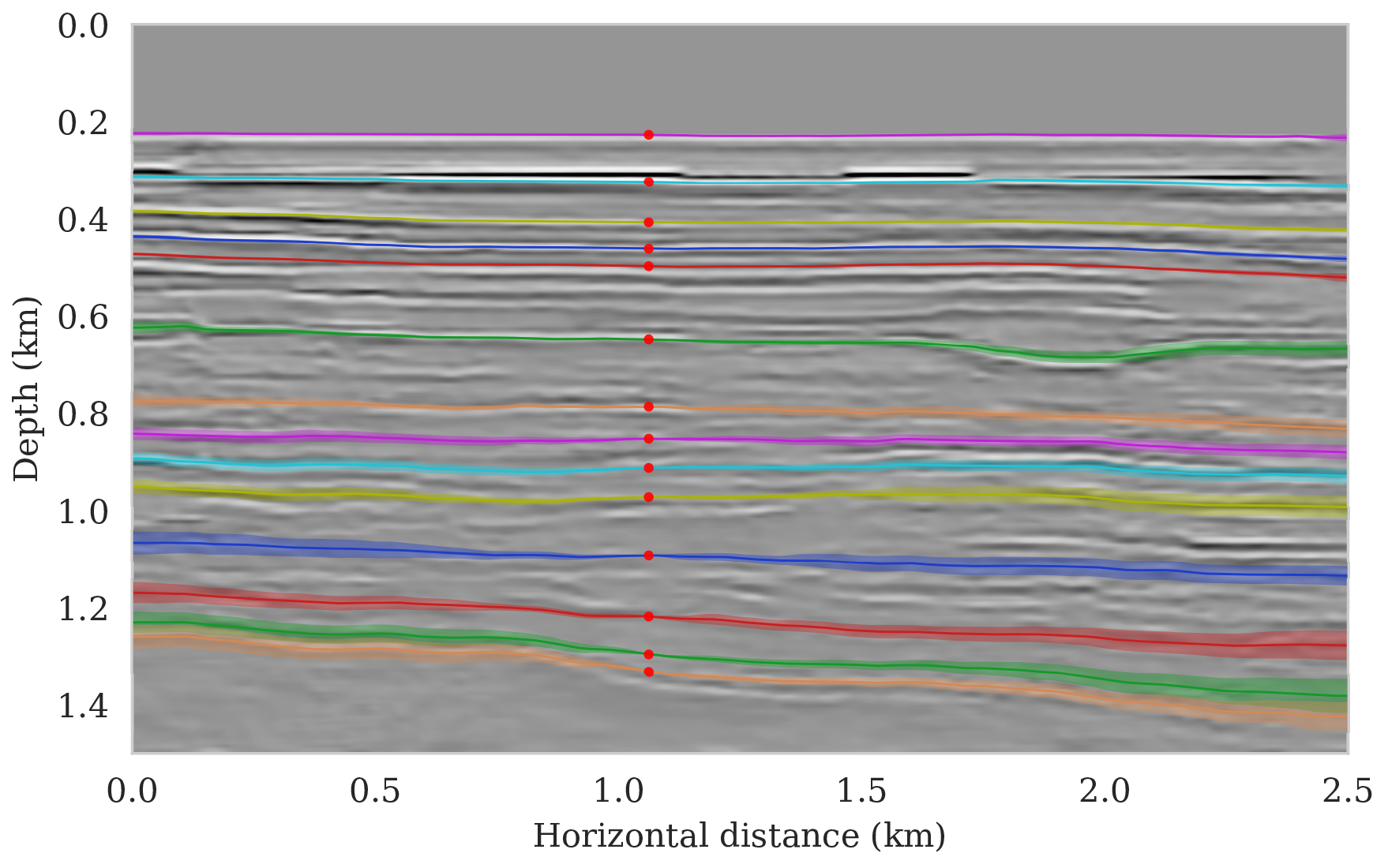
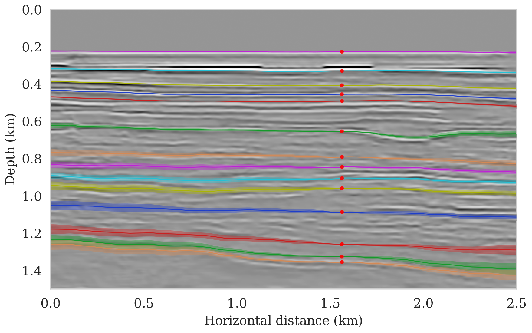
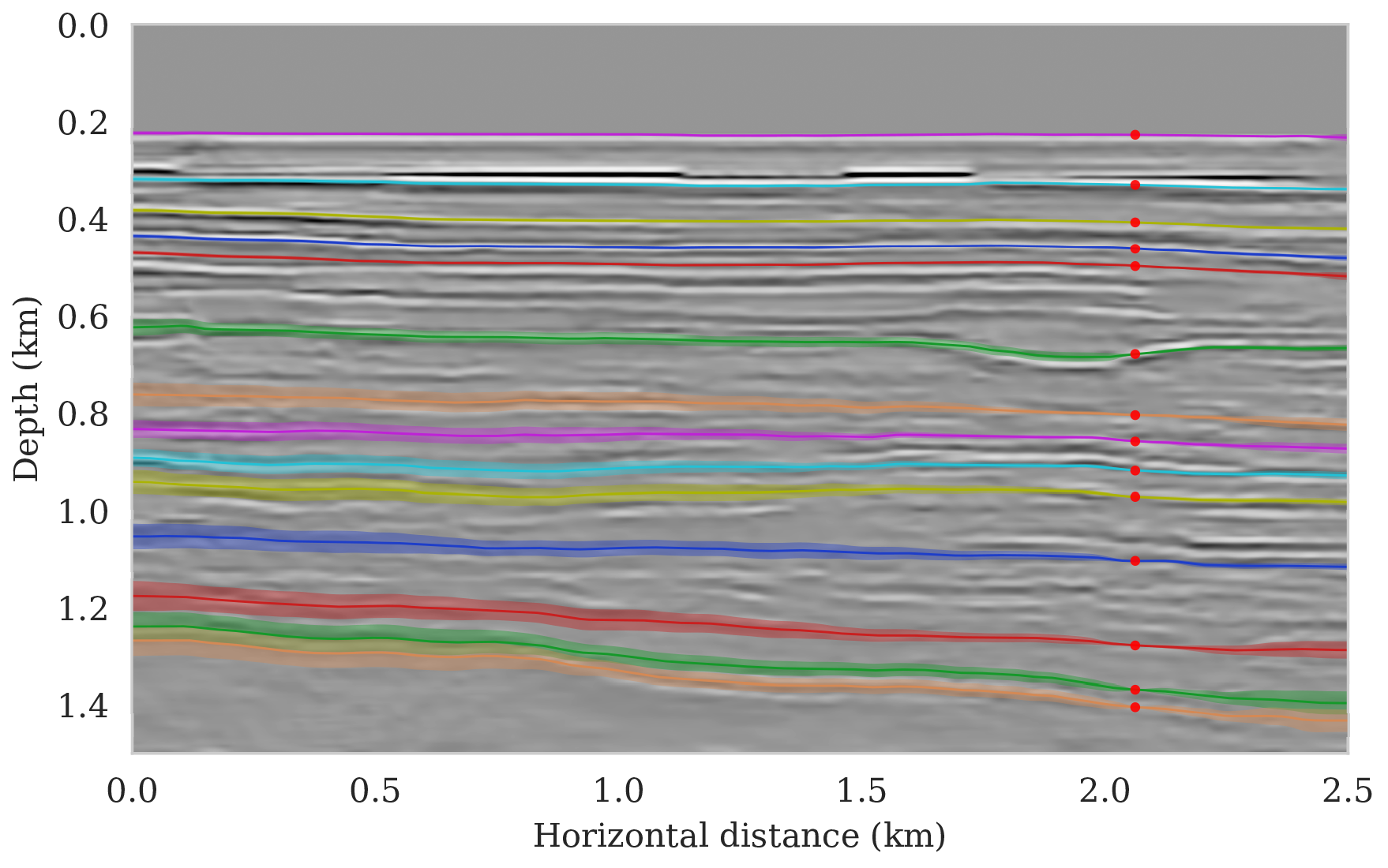
Uncertainty due to noise, linearization errors, and uncertain control points

Following the procedure described above, we also consider the effect of randomness in the horizon tracking task itself. We mimic this by imposing a distribution over the location of control points. As before, we consider the case where we are equally confident in the location of control points. The results for the conditional mean and the \(99\%\) confidence interval are presented in Figure 14. As expected, uncertainties increase consistently with depth, close to the boundaries, and in areas of complex geology. Compared to the previous example, these effects are more pronounced, which we argue is due to an increase in linearization errors at later times in the shot data. This increase leads to more uncertainty in deeper sections.

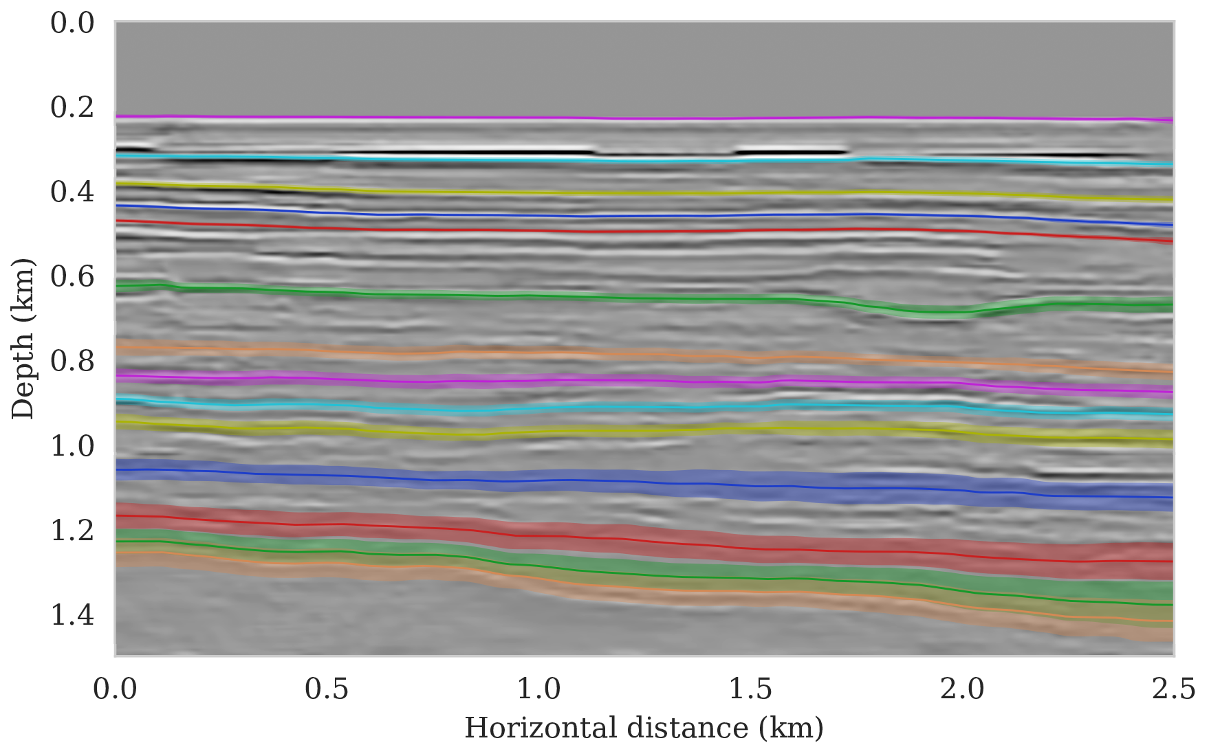
Discussion

The examples presented in this paper demonstrate the beneficial regularization properties of deep priors as long as overfitting of noisy data is avoided. Unfortunately, preventing overfit is challenging in practice. To mitigate this issue, we proposed the use of conditional mean estimates rather than maximum a posteriori (MAP) estimation even though the former relies on sampling the posterior distribution, which is computationally expensive. Based on our experience and other studies (Cheng et al., 2019; Wilson and Izmailov, 2020), estimates based on the conditional mean are comparatively robust to overfitting and yield superior results.

Even though having access to samples from the posterior has many advantages, e.g., it gives us access to the conditional mean and pointwise standard deviation estimates, its computational cost becomes typically prohibitive for large dimensional problems with expensive forward modeling operators. By using techniques from stochastic optimization, we managed to partly offset these costs by avoiding exact calculation of the multi-source data likelihood function. Similar to stochastic optimization, sometimes employed to solve wave-equation based optimization problems (Leeuwen et al., 2011; Haber et al., 2012; Herrmann and Li, 2012b; Lu et al., 2015; Tu and Herrmann, 2015; Chuang Li et al., 2018b), the gradient of the data misfit is calculated for artificially constructed simultaneous source experiments. This reduces the number of wave-equation solves for each gradient calculation significantly. In the context of Langevin dynamics—the theory undergirding our Markov chain Monte Carlo (MCMC) method to sample from the posterior—this stochastic approximation corresponds to the stochastic gradient Langevin dynamics (SGLD) method proposed by Welling and Teh (2011). This approach, in combination with a preconditioning scheme and stepsize schedule, eliminates computationally prohibitive Metropolis-Hasting acceptance steps. By means of several numerical experiments and empirical accuracy measures, we established that the proposed SGLD algorithm is capable of drawing samples from the posterior with a reasonable accuracy. Aside from providing a reasonable assessment of the uncertainty, with pointwise standard deviation increasing in complex areas or in areas of relatively poor illumination, the samples from the posterior also allowed us to propagate uncertainties due to errors in the shot data all the way to the task of automatic horizon tracking or other tasks. With very few exceptions, we are not aware of this type of work on relatively large scale problems (Arnold and Curtis, 2018; Cho and Jun, 2021).

While uncertainty quantification based on Bayesian inference certainly has its merits, it comes at a significant computational price even for 2D problems. These computational costs are compounded by the fact that the parameterization of seismic images in terms of a deep neural network is highly overparameterized, making it more difficult to solve the uncertainty quantification problem. Notwithstanding these challenges, the use of deep priors has several distinct advantages. First, the regularization comes from the inductive bias of the network architecture itself, which is designed to favor natural images. Second, this approach eliminates the need of having access to training data when compared to method that really prior information encoded in pretrained networks. Third, imposing a Gaussian prior on the networks weights is a common regularization strategy (Krogh and Hertz, 1992; Goodfellow et al., 2016). Despite these advantages, the number of iterations needed by the SGLD algorithm remains high and prohibitive for imaging problems in 3D. For this reason, reducing the computational complexity of Bayesian inference over the weights of deep prior networks remains an activate area of research. For instance, Izmailov et al. (2020) proposes to project the network weights onto a low-dimensional subspace and perform posterior inference within this reduced subspace. Unfortunately, construction of this reduced space can also be costly. For the purpose of applying this work to 3D seismic imaging, one possibility is to combine this dimensionality reduction approach with a different form of CNNs that exhibit similar inductive biases to those that we used in this work (Lempitsky et al., 2018) but has fewer weights than the image dimensionality (Heckel and Hand, 2019). As a result, we may be able to exploit the inductive bias of CNNs at a lower computational cost

Despite the fact that Bayesian inference based on MCMC methods, such as SGLD, is well-studied and widely employed, it is challenging for high-dimensional inverse problems that involve expensive forward operator. Variational (Bayesian) inference (Jordan et al., 1999; Rezende and Mohamed, 2015), also known as distribution learning, can potentially overcome these challenges. In this approach, a neural network is trained to synthesize new samples from a target distribution based on a collection of training samples. Typically these samples are obtained by applying a series of learned nonlinear functions to random realizations from a canonical distribution. Early work on variational inference (Rizzuti et al., 2020; Siahkoohi et al., 2020d, 2021; X. Zhang and Curtis, 2020; Kothari et al., 2021; N. Kovachki et al., 2021; Kruse et al., 2021; Kumar et al., 2021; Siahkoohi and Herrmann, 2021; X. Zhao et al., 2021) shows encouraging results, which opens enticing new perspectives on uncertainty quantification in the field of wave-equation based inversion.

Uncertainty in solving (linear) inverse problems including seismic imaging comes in two flavors. On the one hand, there is uncertainty related to noise in the input (shot) data. On the other hand, there may be modeling errors, such as linearization errors, which decrease with the accuracy of the background velocity model. We plan to study how these two types of uncertainty specifically affect the results in future work, with a certain regard for the impact of the background velocity model. Compared to the problem addressed in this paper, this would entail multiple imaging experiments for different background velocity models and is therefore more challenging. Recent developments in full subsurface offset image volumes (M. Yang et al., 2021) and Fourier neural operators (Z. Li et al., 2021) may prove essential in addressing this problem.

Conclusions

Bayesian inference on high-dimensional inverse problems with computationally expensive forward modeling operators, has been, and continues to be a major challenge in the field of seismic imaging. Aside from obvious computational challenges, the selection of effective priors is problematic given the heterogeneity across geological scenarios and scales exhibited by elastic properties of the Earth’s subsurface. To limit the possibly heavy-handed bias induced by a handcrafted prior, we propose regularization via deep priors. During this type of regularization, seismic images are restricted to the range of an untrained convolutional neural network with a fixed input, randomly initialized. Compared to conventional regularization, which tends to bias solutions towards sometimes restrictive choices made in defining these prior distributions, nonlinear deep priors derive regularizing properties from their overparameterized network architecture. The reparameterization of the seismic image by means of a deep prior leads to a Bayesian formulation where the prior is a Gaussian distribution of the weights of the network.

As long as overfitting can be avoided, regularization with deep priors is known to produce perceptually accurate results, an observation we confirmed in the context of controlled seismic imaging experiments. Unfortunately, preventing fitting the noise is difficult in practice. In addition, there is always the question how errors, e.g., bandwidth-limited noise or linearization errors, propagate to uncertainty in the image and to certain tasks to be carried out on the image, which for instance includes the task of automatic horizon tracking. To answer this question and to avoid the issue of overfitting, we propose to sample from the imaging posterior distribution and use the samples to compute the conditional mean estimate, which in our experiments exhibited more robustness to noise, and to obtain confidence intervals for the tracked horizons via our probabilistic horizon tracking framework.

Even though drawing samples from the posterior is computationally burdensome, it allows us to mitigate the imprint of overfitting while it is also conducive to a systematic framework mapping errors in shot data to uncertainty on the image and task at hand. By means of two imaging experiments derived from imaged seismic data volumes, we corroborated findings in the literature that the conditional mean estimate, i.e., the average over samples from the posterior distribution on the image, is more robust to overfitting than the maximum a posteriori estimate. The latter is the product of deterministic inversion. Aside from improving the image quality itself with the conditional mean estimate, access to samples from the posterior also allows us to compute pointwise standard deviation on the image and confidence intervals on automatically tracked horizons.

With few exceptions as of yet, no systematic attempts have been made to account for uncertainties in the task of horizon tracking due to errors in the seismic imaging itself. These errors are caused by noise, linearization approximations, and uncertainty in the horizon tracking process itself, the latter being possibly related to differences in the selection of control points by different interpreters as part of the task of automatic horizon tracking.

To validate the proposed probabilistic tasked imaging framework, we considered realistic scenarios that are representative of two different geological settings. Our findings include: empirical verification of the accuracy of the samples from the posterior distribution; establishment of the conditional mean as a robust estimate for the image; reasonable estimates for the pointwise standard deviation on the image, showing an expected increase in variability in complex geological areas and in areas with poor illumination; and finally confidence intervals for the automatic horizon tracking given the uncertainty on the image and errors in the selection of control points guiding automatic horizon tracking.

Related material

The SGLD iterations (equation \(\ref{sgld}\)) require computing gradient of the negative-log posterior with respect to the CNN weights. This requires actions of the linearized Born scattering operator and its adjoint. For maximal numerical performance, the just-in-time Devito (Luporini et al., 2018; M. Louboutin et al., 2019) compiler was used for the wave-equation based simulations. To have access to the automatic differentiation utilities of PyTorch, we expose Devito’s matrix-free implementations for the migration operator and its adjoint to PyTorch. In this way, we are able to compute the gradients required by equation \(\ref{sgld}\) with automatic differentiation while exploiting Devito’s highly optimized migration and demigration operators. For the CNN architecture, we followed Lempitsky et al. (2018). For the automated horizon tracking we made use of software written by Wu and Fomel (2018). For more details on our implementation, please refer to our code on GitHub.

Acknowledgments

This research was carried out with the support of Georgia Research Alliance and partners of the ML4Seismic Center.

Appendix A

Deep-prior network architecture

The CNN architecture proposed by Lempitsky et al. (2018) is a variation of the widely used U-net architecture, as described by Ronneberger et al. (2015). The U-net architecture is composed of an encoder and a decoder module, where information, i.e., intermediate values, from the encoder module is also passed to the decoder through skip connections.

The following are the major differences between the deep prior architecture (Lempitsky et al., 2018) and the U-net architecture. Contrary to U-net, the convolutional layers in the decoding module of the deep prior architecture do not increase the dimensionality of the intermediate values. Rather, dimensionality-preserving convolutional layers, that is, stride-one convolutions, are augmented with user-defined interpolation schemes to achieve upsampling. This enables the degree of smoothness in the image space to be controlled by the interpolation kernel. Another difference worth noting is the way intermediate values from the encoding phase are incorporated into the decoding module through skip connections. In the deep prior architecture, the intermediate values in the encoding phase are passed through an additional convolutional layer before being fed into the decoder module.

Figure 15 illustrates the exact deep prior architecture used in the Parihaka example in this paper, which closely follows the architecture advocated by Lempitsky et al. (2018). The blocks in the figure represent the intermediate values in the network, where the color indicates the operation that produced these values. For instance, the lightest gray blocks are intermediate values obtained from applying two-dimensional convolutions, whereas the darkest gray block with dashed white edges represents the result of a user-selected interpolation method, which is in this instance nearest neighbor interpolation. For further information regarding the rest of the colors, please refer to the legend in Figure 15. The left most shaded block in Figure 15 is the \(m \times n \times c\) input, which in the case of deep priors is a fixed random array, with \(m,\,n\) indicating its horizontal and vertical dimensions, and \(c\) which represents the number of channels. If a layer alters the dimension of an intermediate value, the new dimensions are inserted adjacent to the representative block. For instance, the leftmost convolutional layer that takes in the input noise changes its dimensionality to \(\frac{m}{2} \times \frac{n}{2} \times 16\). All two-dimensional convolutional layers use \(5 \times 5\) kernels. The convolutional layers that reduce the horizontal and vertical dimensions have a stride of two while all the other convolutional layers have a stride of one. Lastly, we apply a fixed scaler to the output of the network such that the range of the output values for the CNN with fixed input and randomly drawn weights \(\B{w} \sim \mathrm{N} \big (\B{w} \mid \B{0}, \lambda^{-2}\B{I} \big )\) covers the a priori known range of amplitudes in the unknown perturbation model.

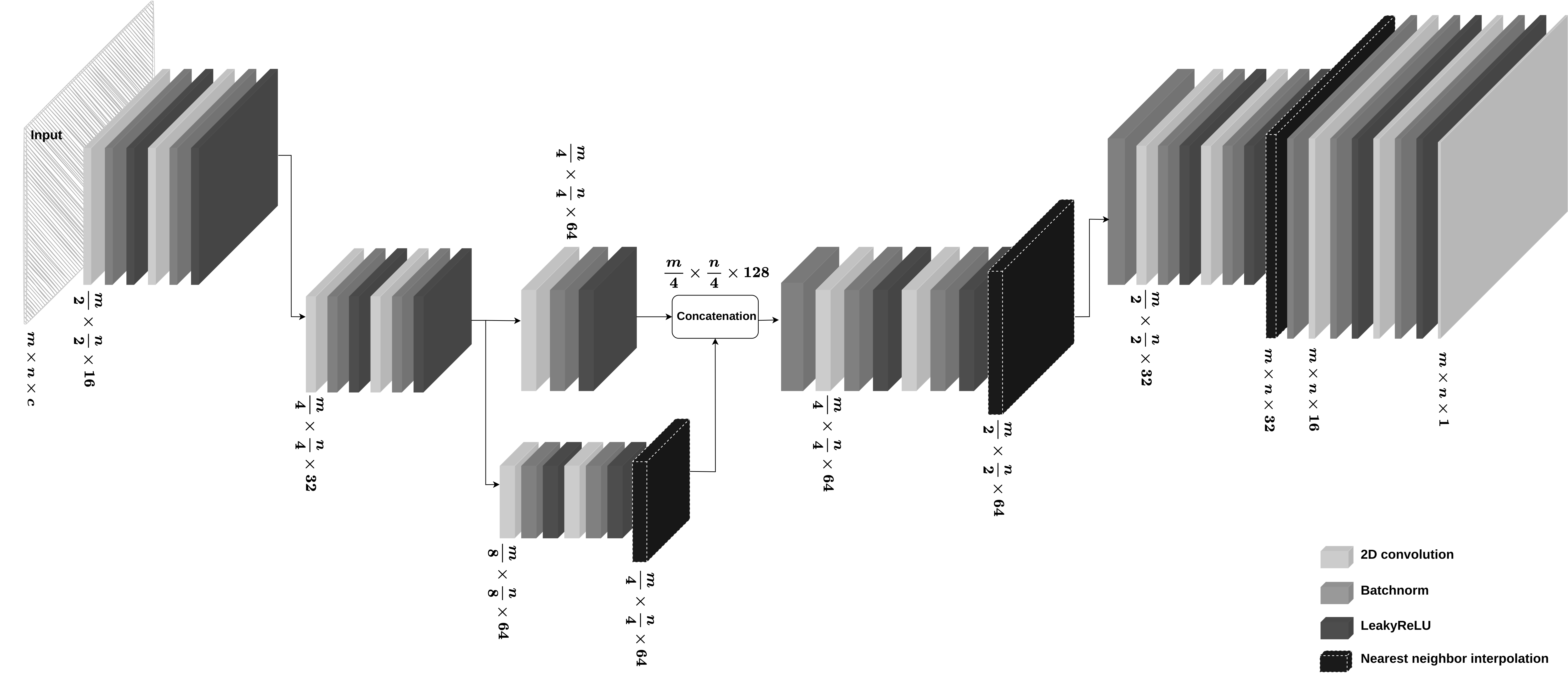
The Compass example uses the same architecture as Figure 15, except that it includes an additional downsampling layer in the encoder and an additional upsampling layer in the decoder. We found the addition of these layers to be helpful since the frequency content of the model in the Compass example was higher and the dimensions larger.

---

1. We use the word “data” interchangeably. In the context of inverse problems “data” refers to observed data. In the context of machine learning data-driven priors refer to priors derived from available samples from an unknown distribution. These are also commonly referred to as “data”. The meaning of the word “data” will be clear from the context.↩

2. \(p(x) = \int_{\mathcal{Y}} p(x, y)\,\mathrm{d}y\), where \(x \in \mathcal{X}\) and \(y \in \mathcal{Y}\) are two arbitrary random variables.↩

3. \(p(x, y) = p(x \mid y)\, p(y), \ \forall\, x \in \mathcal{X},\, y \in \mathcal{Y}\).↩