The importance of transfer learning in seismic modeling and imaging

Ali Siahkoohi, Mathias Louboutin, and Felix J. Herrmann
School of Computational Science and Engineering,  Georgia Institute of Technology
Email: alisk@gatech.edu, mlouboutin3@gatech.edu, felix.herrmann@gatech.edu
Submission date: January 25, 2019

Abstract

Accurate forward modeling is essential for solving inverse problems in exploration seismology. Unfortunately, it is often not possible to afford being physically or numerically accurate. To overcome this conundrum, we make use of raw and processed data from nearby surveys. We propose to use this data, consisting of shot records or velocity models, to pre-train a neural network to correct for the effects of, for instance, the free surface or numerical dispersion, both of which can be considered as proxies for incomplete or inaccurate physics. Given this pre-trained neural network, we apply transfer learning to finetune this pre-trained neural network so it performs well on its task of mapping low-cost, but low-fidelity, solutions to high-fidelity solutions for the current survey. As long as we can limit ourselves during finetuning to using only a small fraction of high-fidelity data, we gain processing the current survey while using information from nearby surveys. We demonstrate this principle by removing surface-related multiples and ghosts from shot records and the effects of numerical dispersion from migrated images and wave simulations.

Introduction

In a perfect world, the wave equation should be able to inform us how to image seismic field data. Often we are met with data behaving erratically or with imaging problems that are too computationally demanding. For these reasons, lots of time and effort has been devoted to wave-equation based imaging technology. We propose to map low-cost low-fidelity solutions to high-fidelity ones whether this involves the free surface or inaccurate numerical wave simulations. Our goal is to do this by using information that is available from nearby surveys.

Several attempts have been made to incorporate machine-learning techniques into seismic processing, imaging, and inversion. Applications range from missing-trace interpolation (Mandelli et al., 2018; A. Siahkoohi et al., 2018) and low-frequency interpolation (H. Sun and Demanet, 2018) to the use of a pre-trained neural network as a prior for full-waveform inversion (Mosser et al., 2018). Ali Siahkoohi et al. (2018) demonstrate the possible application of deep learning in seismic data processing. We extend ideas in Ali Siahkoohi et al. (2018) by utilizing transfer learning to achieve more accurate results by utilizing nearby surveys.

Compared to other imaging modalities, such as medical imaging, we generally do not have access to the ground truth whether this concerns ideal field data or detailed information on the subsurface. This lack of information forces us to fundamentally rethink how to apply machine learning. We combine established data-processing flows with transfer learning (Yosinski et al., 2014). This allows us to map computationally cheap low-fidelity solutions to high-fidelity ones with a pre-trained Convolutional Neural Network (CNN). We train this CNN with data from a survey that is close so that it shares main geological features. Because of its proximity, we assume that this nearby survey and the current survey have similar statistical properties we can use it to pre-train our network. Since this assumption does not hold completely, we use transfer learning to finetune this pre-trained network with a small percentage of data obtained from the current survey. This allows us to replace computationally expensive processing steps with cheaper learned ones, when processing the current survey.

Our paper is organized as follows. First, we describe three approaches for data, gradient, and simulation conditioning designed to deal with cheap low-fidelity simulations. Next, we explain our transfer learning technique, followed by an introduction to Generative Adversarial Networks (GANs, Goodfellow et al., 2014), which we use to map low-fidelity solutions to high-fidelity ones. After describing the used CNN architecture, we demonstrate the capabilities of our approach and the importance of transfer learning on the removal of the effects of the free surface and of a poorly discretized wave equation.

Theory

When solving inverse problems, we implicitly make assumptions on the data. For instance, during seismic imaging we often assume the data to be generated without a free surface, which is not the case in practice. We also assume our simulations as part of imaging free of numerical dispersion, an assumption that may not always be computationally affordable. If these assumptions are violated, wave-equation based inversions will suffer because our simulations will be inconsistent with the observed data. Below we discuss our machine-learning approach to data/gradient/simulation conditioning and how transfer learning and GANs factor into our approach.

Data/gradient/simulation conditioning

Let \(\mathbf{d}_{\text{observed}}\) be the observed data that we try to fit with forward modeling \(F(\mathbf{m} )\) parameterized by the model parameters \(\mathbf{m}\). In the ideal case, \(\mathbf{d}_{\text{observed}}\) is noise free and physically accurate, so \(F\) exactly describes the observed data when \(\mathbf{m}= \mathbf{m} ^{\ast}\) with \(\mathbf{m} ^{\ast}\) the ground-truth model parameters. In that ideal situation, we have \(\mathbf{d}_{\text{observed}} = F(\mathbf{m}^{\ast})\).

As stated before, we usually do not have access to the “true” forward modeling operator, or if we do, its numerical evaluation can be too expensive. Let \(\underline{F}(\mathbf{m})\) denote our low-fidelity forward operator. Given true model parameters \(\mathbf{m}= \mathbf{m} ^{\ast}\), this approximation does not explain the observed data, i.e., \(\mathbf{d}_{\text{observed}} \neq \underline{F}(\mathbf{m}^{\ast})\) and even in the absence of noise, inverting for \(\mathbf{m}\) from observed data will not lead to \(\mathbf{m}^{\ast}\).

To overcome this problem, we propose three different types of conditionings, namely data conditioning, where we take out unmodeled components from the observed data, gradient, and simulation conditioning, where we remove artifacts due to low-fidelity simulations that suffer from numerical dispersion. Because of recent success of CNNs in “image-to-image” mappings (Johnson et al., 2016; Isola et al., 2017), we propose to condition with CNNs, which we train on pairs of low- and high-fidelity simulations. Our examples with numerical dispersion serve as proxies for situations where numerics for the physics may be inadequate. However, we do not claim that our approach is superior to recent work by Amundsen and Pedersen (2019) on removing the effects of temporal dispersion.

Let \(\mathcal{G} _{ \theta_d}\), \(\mathcal{G} _{ \theta_g}\), and \(\mathcal{G}_{ \theta_A}\) be the CNNs used to condition the low-fidelity observed data, gradients, and wavefield simulations, parameterized by \(\theta_d\), \(\theta_g\), and \(\theta_A\), respectively. Mathematically, these conditionings take the following form: \[ \begin{equation} \begin{aligned} \mathbf{d}_{\text{conditioned}} & = \mathcal{G}_{\theta_d} \left ( \mathbf{d}_{\text{observed}} \right ), \\ \end{aligned} \label{data-conditioning} \end{equation} \] \[ \begin{equation} \begin{aligned} \mathbf{g}_{\text{conditioned}} & = \mathcal{G}_{\theta_g}\left( \underline{J}^\top (\delta \mathbf{d})\right),\, \text{and} \\ \end{aligned} \label{gradient-conditioning} \end{equation} \] \[ \begin{equation} \begin{aligned} \mathbf{u}_{\text{conditioned}} & = \mathcal{G}_{\theta_A}\left({\underline{A}^{-1}}\mathbf{q}\right)\\ \end{aligned} \label{simulation-conditioning} \end{equation} \] where \(\mathbf{d}_{\text{observed}}\) represents observed data including the effects of the free surface. The symbol \(\underline{J}\) denotes the low-fidelity Jacobian (linearized Born scattering operator), which acts on \(\delta\mathbf{d}\) the data residual—i.e., observed data after removal of the direct wave. The matrix \(\underline{A}\) corresponds to the low-fidelity discretized wave equation, and \(\mathbf{q}\) to the source. In our examples, \(\mathbf{d}_{\text{conditioned}}\), \(\mathbf{g}_{\text{conditioned}}\), and \(\mathbf{u}_{\text{conditioned}}\) represent shot records without free surface effects, single-shot reverse-time migrations and wavefield snapshots after numerical dispersion removal, respectively.

The above operations are key to iterative wave-equation based inversion where observed data are matched with simulated data. Because each operation involves the wave equation, simulations either miss important physics or are too expensive to evaluate accurately. The key idea now is to condition by training CNNs with pairs of low- and high-fidelity simulations. With these trained CNNs, we map low-fidelity data, gradients, and simulations to high-fidelity ones. We assume that these low- and high-fidelity pairs are available from nearby surveys to pre-train our network.

Transfer learning

Since the Earth subsurface is unknown, finding suitable training sets is often a challenge in the geosciences. We avoid this problem by working with low- and high-fidelity solutions that are both assumed available, e.g. from nearby surveys, albeit the latter often at a higher cost. Generally speaking, we gain if the costs of training and applying the CNNs to the current survey are smaller than the gains we make by avoiding expensive processing, such as the removal of surface-related multiples or conducting accurate high-fidelity simulations. Obviously, this approach can become challenging because of dissimilarities that may exist between the current and nearby surveys. Instead on relying on CNNs to generalize, which may call for massive amounts of training or may not be feasible at all, we rely on transfer learning (Yosinski et al., 2014) to handle the fact that the probability distributions for the nearby and current surveys may not be the same.

During transfer learning, the weights of a pre-trained neural network from the nearby surveys are finetuned to work with data from the current survey. Since transfer learning can be done with a relatively small fraction (\(\approx 5\%\)) of data from the pertinent survey, this can lead to an economically viable workflow since this type of data can often be made available, e.g., by applying more expensive conventional processing on a small fraction of the data of the current survey. Following Long et al. (2015), we avoid overfitting by only finetuning the deeper task-dependent CNN layers during transfer learning. We demonstrate the feasibility of our approach by means of a series of synthetic examples, based on numerical solutions of the wave equation. First, we discuss how we train our networks.

Training objective

Our main goal is to find nonlinear mappings for our three conditioning problems. For this purpose, we use GANs (Goodfellow et al., 2014). This generative approach is capable of training CNNs designed to conduct complex mappings (Johnson et al., 2016; Isola et al., 2017). GANs derive their success from an adversarial training procedure with two CNNs, the generator, which trains to do the mapping, and a discriminator, which trains to distinguish between mapped low-fidelity simulations and true-high-fidelity simulations. We train by minimizing the following two stochastic expectations: \[ \begin{equation} \begin{aligned} \min_{\theta} &\ \mathop{\mathbb{E}}_{\mathbf{x}\sim p_X(\mathbf{x}),\, \mathbf{y}\sim p_Y(\mathbf{y})}\left [ \left (1-\mathcal{D}_{\phi} \left (\mathcal{G}_{\theta} (\mathbf{x}) \right) \right)^2 + \lambda \left \| \mathcal{G}_{\theta} (\mathbf{x})-\mathbf{y} \right \|_1 \right ] ,\\ \min_{\phi} &\ \mathop{\mathbb{E}}_{\mathbf{x}\sim p_X(\mathbf{x}),\, \mathbf{y}\sim p_Y(\mathbf{y})} \left [ \left( \mathcal{D}_{\phi} \left (\mathcal{G}_{\theta}(\mathbf{x}) \right) \right)^2 \ + \left (1-\mathcal{D}_{\phi} \left (\mathbf{y} \right) \right)^2 \right ]. \end{aligned} \label{adversarial-training-expectation} \end{equation} \] The expectations are computed with respect to pairs \(\{\mathbf{x},\, \mathbf{y}\}\) of low- and high-fidelity images drawn from the probability distributions \(p_X (\mathbf{x})\) and \(p_Y (\mathbf{y})\). By alternating the above minimizations, we simultaneously train the generator \(\mathcal{G}_{\theta}\) to create a low-to-high fidelity map and the discriminator \(\mathcal{D}_{\phi}\) to discern the low-to-high fidelity map from a true high-fidelity one. Following Isola et al. (2017), we include an additional \(\ell_1\)-norm misfit term weighted by \(\lambda\). This term is designed to ensure that each realization of \(\mathcal{G}_{\theta}(\mathbf{x})\) maps to a particular \(\mathbf{y}\)—i.e., \(\mathbf{x}\mapsto\mathbf{y}\) rather than solely fooling the discriminator.

We minimize the above objectives with a variant of Stochastic Gradient Descent known as the Adam optimizer (Kingma and Ba, 2014) with momentum parameter \(\beta = 0.9\) and a linearly decaying stepsize with initial value \(\mu = 2 \times 10^{-4}\) for both the generator and discriminator networks. During each iteration of Adam, the expectations in the above expressions are approximated by evaluations of the objective value and gradient for a single randomly selected training pair. These pairs are selected without replacement.

CNN architecture

“Image-to-image” mappings typically call for a hierarchical neural network consisting of encoder-decoder neural networks (Isola et al., 2017; Johnson et al., 2016). Since the low- and high-fidelity data share a lot of information, we use CNNs that contain skip connections that exploit similarities, which allows for faster convergence during training (He et al., 2016). We used the exact architecture provided by Johnson et al. (2016), which includes Residual Blocks, the main building block of ResNets, introduced by He et al. (2016), for the generator \(\mathcal{G}_{\theta}\). For the discriminator \(\mathcal{D}_{\phi}\), we utilize the “PatchGAN” architecture, exactly as it was introduced by Isola et al. (2017). We designed and implemented our deep architectures in TensorFlow¹. To carry out our wave-equation simulations with finite differences, we used Devito² (Louboutin et al., 2018; Luporini et al., 2018).

Numerical experiments

Wave-equation based imaging relies on the assumption that observed data and simulations are consistent, which is often not the case. To handle this situation, we demonstrate how CNNs can be used to remove the effects of the free surface and numerical dispersion. Our data conditioning partly replaces the numerically expensive process of SRME (Verschuur et al., 1992) and deghosting by the action of a transfer-trained CNN that removes the imprint of the free surface. In the second and third examples, we correct migrated shot records and wave simulations by CNNs trained to correct numerical dispersion.

Surface-related multiple elimination and deghosting

While wave-equation based techniques for removing the free surface are applied routinely, these techniques are computationally expensive and often require dense sampling. Here, we follow a different approach where we train a CNN to carry out the joint task of surface-related multiple removal and source-receiver side deghosting.

Specifically, we consider the situation where we have access to pairs of shot records from a neighboring survey before and after removal of the free-surface effects through standard processing. These pairs of unprocessed and processed data allow us to pre-train our CNN. To mimic this realistic scenario, we simulate pairs of shot records with and without a free surface for nearby velocity models that differ by \(25\%\) in water depth. These pairs, which correspond to changes in water depth by \(50\) \(\mathrm{m}\), are used to pre-train our network. We make this choice for demonstration purposes only, other more realistic choices are possible. We simulate our marine surveys with a Ricker wavelet centered at \(50\) \(\mathrm{Hz}\) and with sources and receivers towed at a depth of \(9\) \(\mathrm{m}\) and \(14\) \(\mathrm{m}\), respectively.

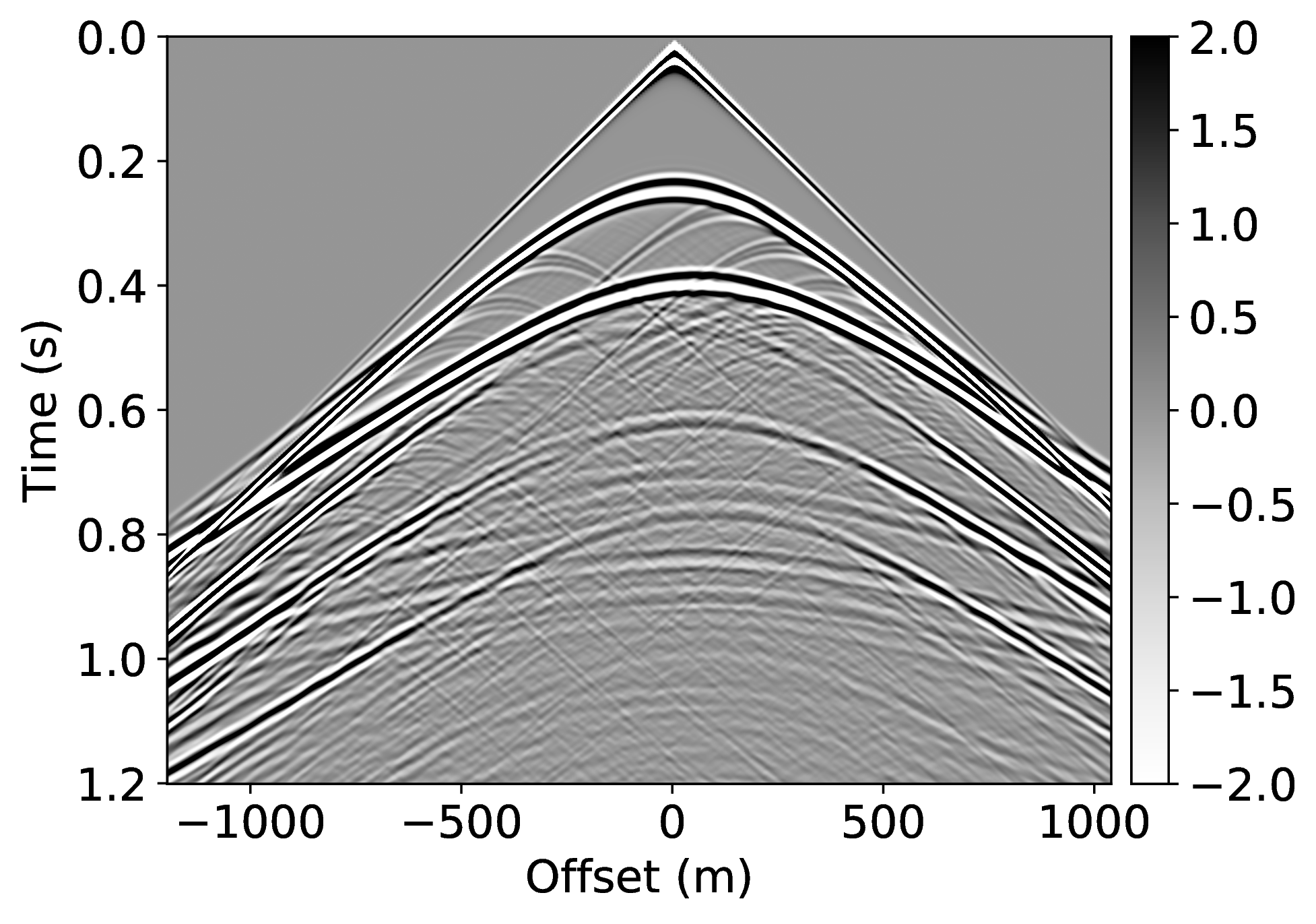
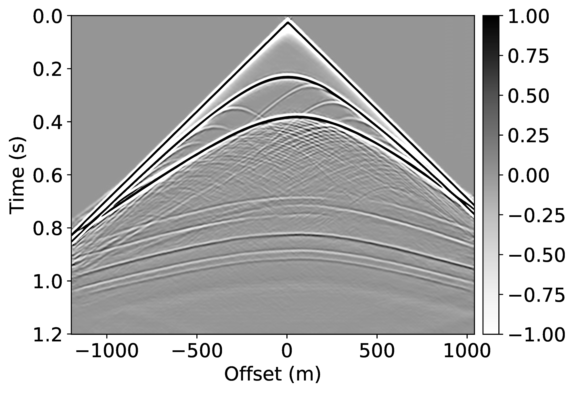
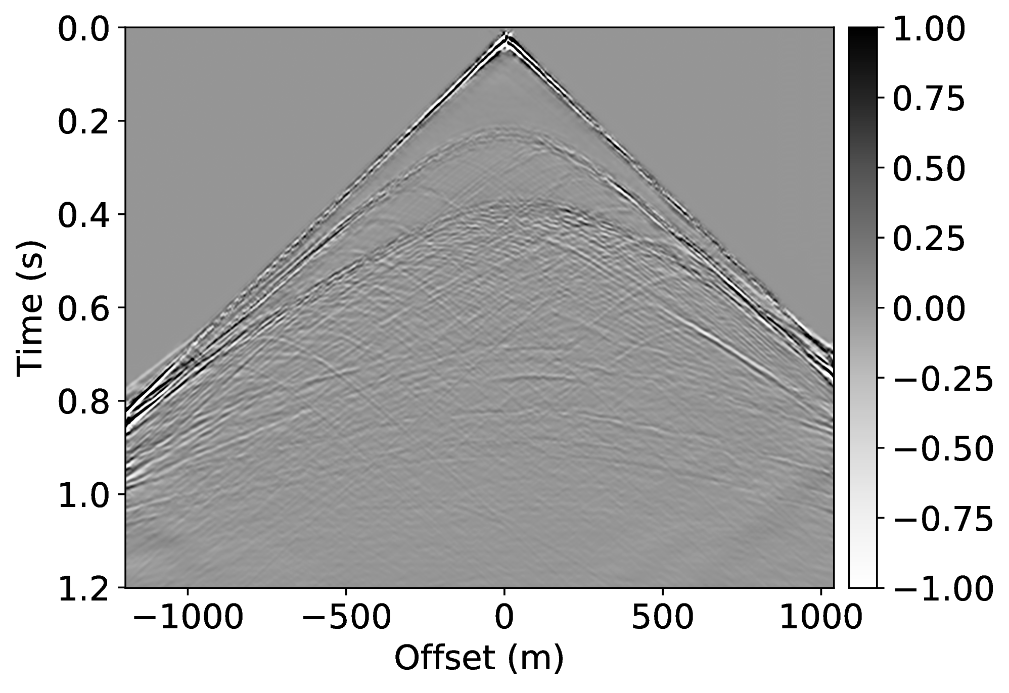
Because the water depth between the nearby and current surveys differ by \(25\%\), we finetune our CNN on only \(5\%\) of unprocessed/processed shot records from the current survey—i.e., we only process a fraction of the data. We numerically simulate this scenario by generating shot records in the true model (correct water depth) with and without a free surface. While this additional training round requires extra processing, we argue that we actually reduce the computational costs by as much as \(95\%\) if we ignore the time it takes to apply our neural network and the time it takes to pre-train our network on training pairs from nearby surveys. In Figure 1, we present our result for a shot record not seen during training. We obtained this result by applying Equation \(\ref{data-conditioning}\) with a CNN trained by minimizing objectives \(\ref{adversarial-training-expectation}\) for \(\lambda = 1000\) with \(100\) passes through \(802\) shot records from the nearby surveys, followed by a round of transfer learning involving \(100\) passes over only \(21\) shot records of the current survey. We found the value for \(\lambda\) after extensive parameter testing. During the selection of the \(\lambda\)-value, we made sure that the output of the discriminator averages in the end to \(\frac{1}{2}\) (by choosing \(\lambda\) not too large). We also made certain that the training pairs map one-to-one (by choosing \(\lambda\) large enough). As reported in the literature by Hu et al. (2019), training results typically vary not by much when varying this parameter. Our results confirm the ability of a (pre-)trained neural network to remove both surface-related multiples and ghosts (cf. Figures 1c and 1d). We carried out this training by using data from nearby surveys followed by transfer training on a small number of data pairs from the current survey during transfer training.

Numerical dispersion removal

To demonstrate how CNNs handle incomplete and/or inaccurate physics, we consider two examples where we use a poor discretization (only second order) for the Laplacian. Because of this choice, our low-fidelity wave simulations are numerically dispersed and we aim to remove the effects of this dispersion by properly trained CNNs. For this purpose, we first train a CNN on pairs of low- and high-fidelity single-shot reverse-time migrations from a background velocity model that is obtained from a “nearby” survey. We perform high-fidelity simulations by using a more expensive \(20^{\mathrm{th}}\)-order stencil. Secondly, we correct wave simulations themselves with a neural network that is trained on a family of related “nearby” velocity models. Both examples are not meant to claim possible speedups of finite-difference calculations. Instead, they are intended to demonstrate how CNNs can make non-trivial corrections such as the removal of numerical dispersion.

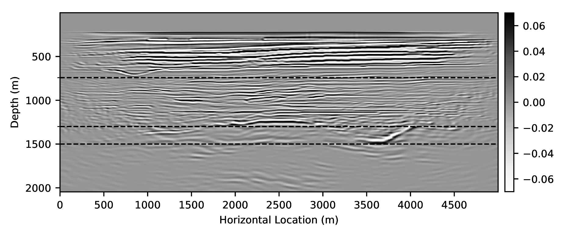
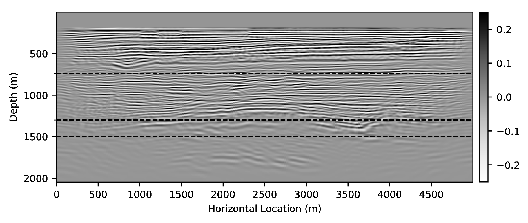
As an example of gradient conditioning, we pre-train a CNN by minimizing objectives \(\ref{adversarial-training-expectation}\) with \(\lambda = 100\) for \(100\) passes over \(804\) pairs of low- and high-fidelity single-shot reverse-time migrations simulated for four “nearby” surveys defined by four different vertical 2D slices taken from the 3D BG Compass velocity model. As before, we find the value for \(\lambda\) via extensive parameter testing. Because these 2D slices are different from the current velocity model, we need to transfer train. We do this by carrying out an additional training round via \(20\) passes over only \(11\) low- and high-fidelity gradient pairs. This means we only migrate \(5\%\) of the shots high-fidelity in the current velocity model. After this two-stage training procedure, we apply corrections to numerically dispersed gradients computed for the current model. Figure 2 depicts the results of these gradient corrections. While the low-fidelity migrations contain large errors in positioning and amplitudes, our transfer-trained CNN corrects these errors, see for instance along the dotted lines in Figure 2, horizontal locations \(800\) \(\mathrm{m}\), \(2500\) \(\mathrm{m}\), and \(3700\) \(\mathrm{m}\).

In the final experiment, we remove numerical dispersion from low-fidelity wave simulations. We follow H. Sun and Demanet (2018) and crop five pieces of the Marmousi model so that their size is reduced to \(10\%\) of the original model. To make the size the same as the original model, we interpolate the selected subsets. We generate from these models low- and high-fidelity wavefield pairs for various time-steps and source positions.

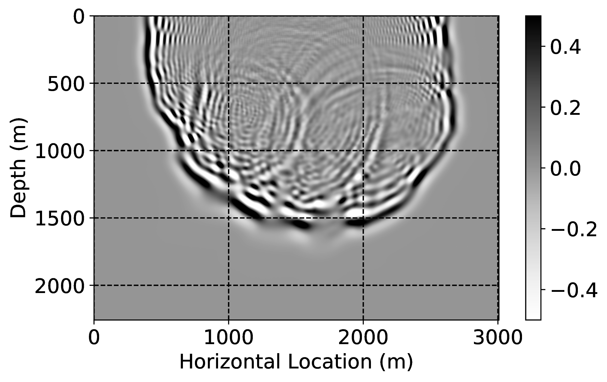
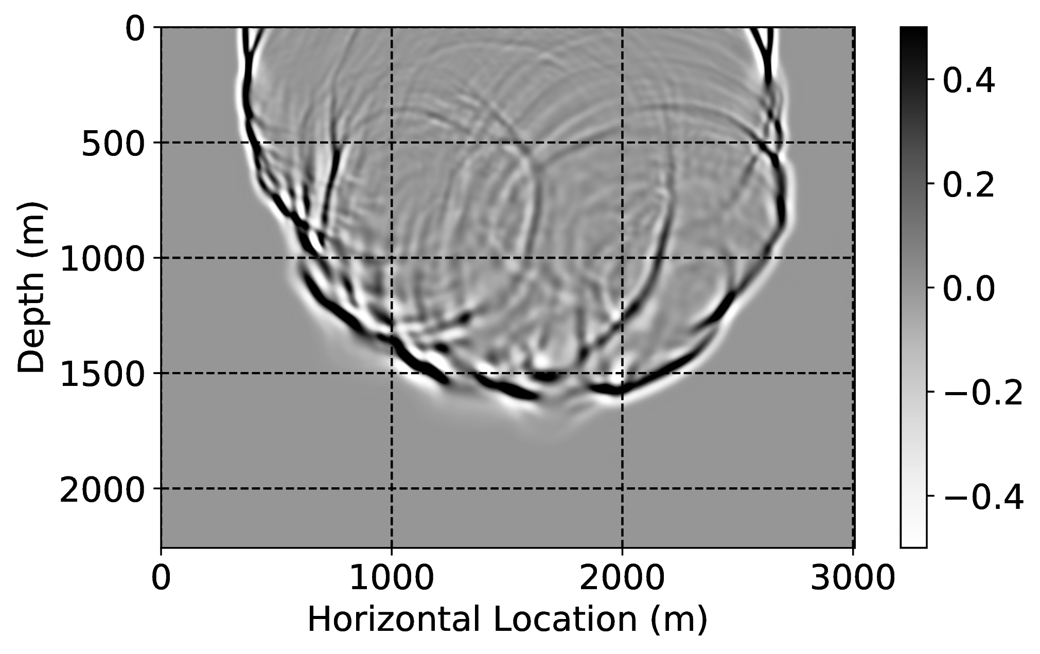
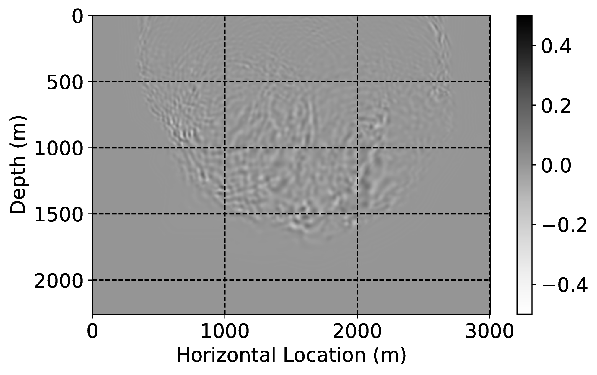
We train a CNN by minimizing objectives \(\ref{adversarial-training-expectation}\) for \(5 \times 401 \times 11 =22055\) low- and high-fidelity wavefield snapshots simulated on these five training velocity models at \(401\) source locations and \(11\) randomly selected time snapshots. Since the cropped velocity structures are less complex than the original velocity model, an additional round of transfer learning is required. We finetune the CNN by training on \(1500\) (\(5\%\)) low- and high-fidelity snapshot pairs. For training, we use \(\lambda = 100\) in objectives \(\ref{adversarial-training-expectation}\) and we made \(4.5\) passes through the full data set (i.e., we touch all shots four times and half of them five times) followed by \(11\) passes during transfer learning. Figure 3 depicts the results of the wavefield corrections. While the low-fidelity wave simulations show a heavy imprint of numerical dispersion, e.g., strong phase and amplitude distortions, the result depicted in Figure 3c, demonstrates that the CNN has mostly corrected these errors. As we stated before, we do not claim to improve on recent work by Amundsen and Pedersen (2019) with this example. We only want to demonstrate that CNNs can be used for this purpose.

Conclusions

We showed that pre-trained convolutional neural networks (CNN), trained via an adversarial objective function introduced by generative adversarial networks, can conduct complex tasks including removal of the free surface and mitigation of the effects of numerical dispersion during reverse-time migration and wave simulations. We were able to this by exposing our CNNs to only a small percentage of training data pertinent to the task at hand. Our experiments are exclusively based on numerical simulations. They demonstrate that as long as we are able to pre-train the neural network, e.g., by using data from a neighboring survey or by wave simulations in related velocity models, we can get good performance after finetuning this network with only a few low- and high-fidelity pairs pertinent to the current model. We argue that this may lead to future improvements in efficiency where computationally expensive (e.g., wave-equation driven) processing can partly be replaced by a potentially numerically more efficient neural network. Even though seismic data processing and imaging may differ significantly from location to location, seismic waves and Earth models do share information allowing us to pre-train neural networks by priming them for transfer learning. By following this approach, we rely less on generalizability of our CNNs and more on the availability of information from nearby surveys.

So far, our results are limited to two-dimensional image-to-image mappings, applied to numerically modeled data, and the challenge will be to scale these mappings to higher dimensions. Key in this development will be the ability of these neural networks to generalize sufficiently so that the cost of transfer learning remains small enough.

---

1. https://www.tensorflow.org/↩

2. https://www.devitoproject.org/↩