Geological Carbon Storage

gcs

SLIM Team

Introduction

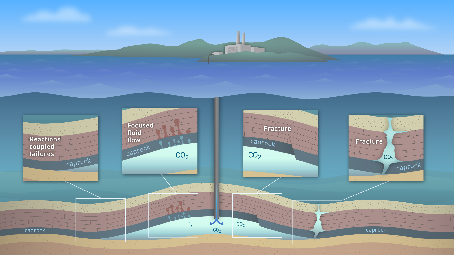
Geological Carbon Storage (GCS) is an essential technology to help mitigate risks of climate change. To meet the goals of the Paris Agreement (Rockström et al. 2017), it is estimated that 550 million tons (Mt) of CO₂ must be sequestered per year by 2030 and 5,500 Mt CO₂ by 2050, which corresponds to a need of approximately 12,000 CO₂ injection sites globally by 2050 P. Ringrose (2020). While GCS is a promising technology to inject large amounts of supercritical CO₂ into rock formations for long-term storage, there may be certain risks associated with this technology that call for reassurance of the public, regulators, and other stakeholders of its safety. Even for well-designed CO₂ injection projects with accurately established baselines, there remains a risk that the CO₂ plume leaves the storage complex via e.g. focused fluid flows, porosity collapse, or changes in fracture networks. An illustration of this is shown in Figure 1 below.

Figure 1: Illustration of different leakage scenarios of Geological Carbon Storage (GCS)

At the Seismic Laboratory for Imaging and Modeling (SLIM), and as part of the industry partners program ML4Seismic, we are addressing these risks by embracing recent developments in simulation-based Bayesian inference (Cranmer, Brehmer, and Louppe 2020)—i.e., the task of deriving statistical information from a system based on in silico simulations—that allows us to develop low-cost, scalable, high-fidelity and uncertainty-aware seismic monitoring solutions for GCS. Our envisioned approach consists of the following components:

Simulation-based monitoring design—a capability to generate realistic time-lapse data in response to CO₂ injection in large strongly heterogeneous reservoirs, e.g. saline aquifers;
Seismic monitoring with the joint recovery model—an inversion framework capable of producing high-fidelity time-lapse images of CO₂ plumes from sparse non-replicated time-lapse data collected in response to CO₂ injections;
Deep neural network classifiers for CO₂ leakage detection—a Class Activation Mapping (CAM) framework to identify areas of possible CO₂ leakage from imaged time-lapse seismic data;
Surrogate end-to-end inversion—a coupled inversion framework that produces estimates for the permeability from time-lapse seismic data using Fourier neural operators as surrogates for two-phase flow;
Scalable parallel domain-decomposed Fourier neural operators—high-performance computing implementation of 3D Fourier neural operators;
Uncertainty-aware Digital Twin for Geological Carbon Storage—a data-assimilation framework based on simulation-based Bayesian and sequential Bayesian inference capable of rapidly producing high-fidelity CO₂ plume forecasts that are consistent with observed time-lapse seismic data;

Simulation-based monitoring design

While various monitoring modalities exist to track the behavior of CO₂ plumes to ensure safe operations and compliance with regulatory requirements, active 3D time-lapse seismic monitoring has proven superior but costly. At SLIM, we aim to reduce the operating costs by optimizing acquisition design and to answer questions such as

How often and when (early and/or late in a GCS projects) do seismic surveys need to be performed to mitigate long-term risks?
How can the sensitivity of seismic monitoring systems be improved while keeping costs down?
To what degree do time-lapse surveys have to be replicated to achieve high degrees of repeatability?

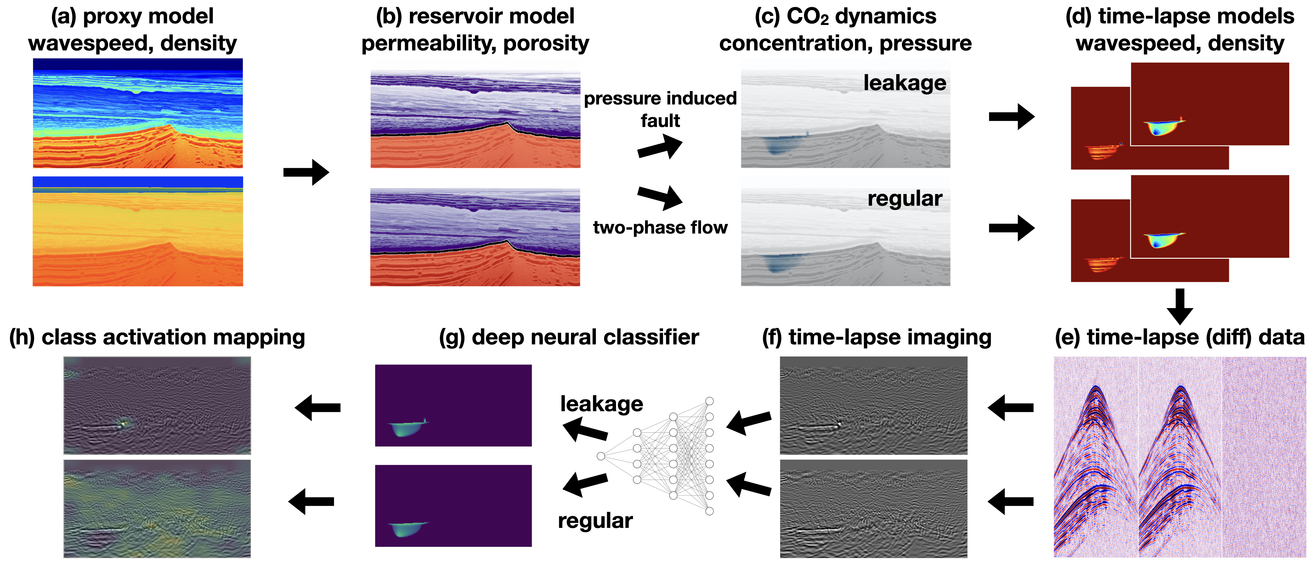
Animation1Example of our Simulation-based monitoring framework implemented with Seis4CCS.jl

To answer these questions and to help drive innovations in seismic monitoring acquisition design and imaging, we are developing an open-source software platform Seis4CCS.jl that allows users to perform simulation-based monitoring design and test novel time-lapse acquisition and imaging technologies in silico at scale. An example of our simulation-based framework is included in Animation 1. This example is based on the Compass model (Jones et al. 2012). This model, which is derived from real imaged 3D seismic and well-log data, is representative of the geology of saline aquifers in the southwest corner of the North Sea. To create realistic CO₂ plumes, we convert this synthetic seismic proxy model of the compressional wavespeed and density to a proxy model of the porosity and permeability. For this conversion, we make use of empirical relationships derived in (Klimentos 1991).

As outlined in the Strategic UK CCS Storage Appraisal Project report, the stratigraphic sections in this model can be roughly divided into three main sections, namely:

The reservoir, consisting of highly porous (average 22%) and permeable ( > 170 mD) Bunter Sandstone of about 300 − 500 m thick (red area in the second plot of the top row of Animation 1);
The primary seal, (permeability 10⁻⁴ − 10⁻² mD) made of the Rot Halite Member, which is 50 m thick (black layer in the second plot of the top row of Animation 1);
The secondary seal, made of the Haisborough group, which is > 300 m thick and consists of low-permeability (15 − 18 mD) mudstone (blue area in the second plot of the top row of Animation 1).

Given these proxy models of fluid-flow properties, we simulate the injection of supercritical CO₂ using the open-source software FwiFlow.jl (D. Li et al. 2020). This code simulates the growth of CO₂ plumes by solving the subsurface two-phase flow equations. To mimic CO₂ leakage due to a pressure induced opening of a fault, we increase the permeability at a given location when the induced pressure reaches a critical threshold. Animation 1 shows a movie of the plume development in a leakage scenario.

After fluid-flow simulation, the time-varying CO₂ concentration is converted to changes in the compressional wavespeed and density via the patchy saturation model (Avseth, Mukerji, and Mavko 2010). These time-lapse changes in seismic properties are localized at the plume location and are then used to generate synthetic time-lapse seismic datasets with and without leakage. These datasets then serve as input to the joint recovery model (JRM) and neural network based leakage classifiers. Additionally, these simulated seismic datasets will become part of a series of benchmarks designed to test and compare the performance of different approaches to seismic monitoring.

Seismic monitoring with the joint recovery model:

Time-lapse seismic monitoring is widely used to monitor the CO₂ dynamics in GCS projects (Lumley 2001; Chadwick et al. 2010). Despite its wide use, seismic monitoring is challenging because time-lapse differences are often relatively small in extent and amplitude, which implies they call for high-fidelity (and therefore costly) imaging of the baseline and monitor surveys. To avoid misidentification of CO₂ plumes due to artifacts, the recovered images also need to be highly repeatable in order for subtle CO₂-induced time-lapse changes to be detected, e.g. by computing differences between the baseline and monitor surveys or between the monitor surveys themselves.

To improve the repeatability of the recovered images without insisting on costly and challenging replication of the monitoring surveys, use is made of the joint recovery model (JRM) (Oghenekohwo et al. 2017; Wason, Oghenekohwo, and Herrmann 2017). Contrary to conventional approaches, where time-lapse seismic datasets are imaged separately, the JRM inverts for the common component, which captures information shared amongst different surveys, and for time-lapse innovations with respect to this common component. This novel inversion approach has been deployed successfully to several time-lapse recovery problems, including but not limited to wavefield reconstruction from sparse simultaneous source acquisition (see Acquisition tab) (Oghenekohwo et al. 2017; Wason, Oghenekohwo, and Herrmann 2017; Oghenekohwo and Herrmann 2017), imaging, full-waveform inversion (Oghenekohwo 2017; Z. Yin, Louboutin, and Herrmann 2021), and field data denoising (Wei et al. 2018).

Mathematically, the JRM for n_v different monitoring surveys involves inverting the following matrix:

$$ \mathbf{A} = \begin{bmatrix} \frac{1}{\gamma} \nabla\mathcal{F}_1(\mathbf{\overline{m}}_1) & \nabla\mathcal{F}_1(\mathbf{\overline{m}}_1) & & \\ \vdots & & \ddots & \\ \frac{1}{\gamma} \nabla\mathcal{F}_{n_v}(\mathbf{\overline{m}}_{n_v}) & & & \nabla\mathcal{F}_{n_v}(\mathbf{\overline{m}}_{n_v}) \end{bmatrix}, \qquad(1)$$

where each ∇ℱ_k, k = 1⋯n_v denotes the linearized Born modeling operator for a given vintage, parameterized by the corresponding background model, $\mathbf{\overline{m}}_k$. This matrix relates the common component (z₀) and innovation components (z_k), collected in vector z = [z₀, z₁, ⋯, z_{n_v}]^⊤, to the linearized time-lapse datasets collected in vector δd = [δd₁, ⋯, δd_{n_v}]^⊤. This linear system of equations can be inverted via the linearized Bregman method (W. Yin et al. 2008; Witte et al. 2019; Yang et al. 2020). After inverting this system, the seismic monitoring images for each vintage x_k are computed by summing the common and innovation components—i.e., $\frac{1}{\gamma} \mathbf{z}_0 + \mathbf{z}_k, k=1\cdots n_v$.

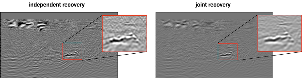
Figure 2: Comparison of joint recovery (left) and independent recovery (right) results. The CO₂ leakage over the seal is located at 2500 m lateral position.

The seismic images recovered by JRM are more repeatable compared to the images recovered by independent imaging, yielding lower NRMS values (Kragh and Christie 2002). Check this SEG 2021 abstract and the GitHub Repository for more information.

Deep neural network classifiers for CO₂ leakage detection

SLIM’s ultimate goal is to detect potential CO₂ leakage out of the storage complex from time-lapse seismic monitoring data. To this end, we propose a deep-learning binary classification methodology to automatically detect potential CO₂ leakage due to pressure-induced activation of pre-existing faults from time-lapse seismic data. Aside from determining whether the CO₂ plume develops regularly or not (i.e. sealed or leakage), we also employ Class Activation Mapping (CAM) methods (Zhou et al. 2016) to generate saliency maps to visualize areas in the time-lapse seismic image that are crucial to the model classification result. Compared to our earlier work on Simulation-based monitoring design and Seismic monitoring with the joint recovery model, this classification process required an additional step as illustrated in Figure #fig-cam-framework below).

Figure 3: Diagram for simulation-based monitoring with deep neural network classifiers for leakage detection

For comparison, we use 4 different types of classification network models, including ResNet34 (He et al. 2016), VGGNet16 (Simonyan and Zisserman 2014), Vision Transformer (ViT) (Vaswani et al. 2017) and Shifted Window Transformer (Swin) (Liu et al. 2021). Predicted accuracy on unseen seismic images obtained from time-lapse seismic datasets are included in table below while Figure Figure 4 contains the CAM-based saliency maps.

Model	Accuracy	Precision	Recall	F1	ROC-AUC
VGG16	0.920 ± 0.089	0.941 ± 0.133	0.921 ± 0.081	0.927 ± 0.075	0.920 ± 0.076
ResNet34	0.948 ± 0.020	0.982 ± 0.028	0.928 ± 0.044	0.948 ± 0.040	0.967 ± 0.019
ViT	0.857 ± 0.018	0.910 ± 0.102	0.820 ± 0.098	0.859 ± 0.036	0.923 ± 0.023
Swin	0.836 ± 0.036	0.881 ± 0.108	0.818 ± 0.078	0.841 ± 0.076	0.909 ± 0.007

Figure 4: CAM saliency maps. The highlighted regions indicate potential CO₂ leakage.

From these CAM maps, we observe that the ViT structure with Score-CAM has the narrowest highlighted region that shows the CO₂ leakage. These classification results and CAM saliency maps can be used by practitioners to alert the early stages of potentially anomalous CO₂ plume development during GCS projects. More information can be found in this 2022 manuscript.

Surrogate end-to-end inversion

While time-lapse monitoring using the joint recovery model yields seismic images with a high degree of repeatability without insisting on replication of the time-lapse surveys, it does not provide direct access to the fluid-flow properties, i.e., the permeability and porosity distribution within the reservoir. Improving our understanding of the spatial distribution of permeability forms an essential component of measurement, monitoring and verification (MMV) of GCS projects that call for accurate modeling of CO₂ plume dynamics. To gain access to the spatial permeability distribution from observed time-lapse seismic data, we follow recent work by D. Li et al. (2020) where the seismic forward model is coupled to the physics of two-phase flow. This coupling can then be used to invert for the intrinsic permeability of the reservoir.

In an effort to improve the inversion results and prepare for integration with uncertainty-aware problem formulations, recent developments in surrogate modeling via deep neural networks are employed in a two-pronged approach wherein both the physics of two-phase flow and the statistical distribution of permeability are captured by a neural network. Following Z. Li et al. (2020), we train a Fourier neural operator (FNO) to learn time-varying solutions of the two-phase flow equations for corresponding spatially varying samples of the permeability drawn from a specific distribution. This training process learns the mapping K ↦ 𝒮_θ(K) where K represents the spatially varying permeability and 𝒮_θ(⋅) the trained FNO with network weights θ. After converting the CO₂ concentration to changes in the compressional wavespeeds and seismic forward modeling (via the operators ℛ and ℱ), this mapping can be used to invert for the permeability from time-lapse seismic data by minimizing

$$ \underset{\mathbf{z}}{\operatorname{minimize}} \quad \frac{1}{2}\|\mathcal{F}\circ\mathcal{R}\circ\mathcal{S}_{\boldsymbol{\theta}}\left(\mathbf{K}\right)-\mathbf{d}\|_2^2 \quad \text{subject to}\quad \mathbf{K}=\mathcal{G}_{\mathbf{w}}(\mathbf{z}). \qquad(2)$$

In this expression, 𝒢_w represents a normalizing flow trained to generate spatially varying samples from the permeability distribution given the latent variable z.

Figure 5: Diagram for surrogate end-to-end inversion (cf. Equation #couple) where the symbols ℱ, ℛ, 𝒮_θ represent the wave, rock, and fluid-flow physics respectively. The latter is represented by a trained Fourier neural operator (FNO) that acts as a surrogate for two-phase flow

Because 𝒢_w is trained to generate samples from the permeability distribution, adding it as a constraint acts as a regularizer on the ill-posed inversion problem for the spatial permeability distribution. Figure #fig-end2end-result contains an example of end-to-end inversion by solving the optimization problem defined in #couple. Because of buoyancy effects, the injected CO₂ plume (see also Figure #fig-end2end-framework (a)) does not occupy the deeper part of the model, causing errors in the estimated permeability for deeper parts of the model (see the top row of Figure #fig-end2end-result). Despite these errors, the predicted CO₂ plumes are quite accurate (see Figure #fig-end2end-framework (b)). Furthermore, the inverted permeability can be used to forecast the growth of CO₂ plumes in the future at a near-zero additional cost via forward evaluation of the FNO. We observe that the forecast is relatively accurate and catches the global behavior of the plume even though no seismic monitoring data is available (see Figure #fig-end2end-framework (c)). More information can be found in the SEG 2022 abstract and FNO4CO2.jl.

Figure 6: End-to-end inversion from 11 seismic surveys with FNO as a surrogate. (a) Initial, inverted and true permeability. (b) 4 rows (from top to bottom) are initial, predicted, true CO₂ saturation snapshots and 5× error. (c) 4 rows (from top to bottom) are initial, forecasted, true CO₂ saturation snapshots and 5× error. These CO₂ saturation snapshots are forecasted by FNO without any available seismic data.

Scalable parallel domain-decomposed Fourier neural operators

The efficacy of the aforementioned end-to-end inversion framework on large-scale CO₂ monitoring hinges upon the capability to scale FNOs. To fight the curse of dimensionality, we propose a model-parallel version of FNOs based on domain-decomposition of both the input data and the network weights (Grady II et al. 2022). A sketch of the distributed FNO block structure is shown in Figure #fig-dfno. In collaboration with Microsoft Research and Extreme Scale Solutions, we demonstrate that our model-parallel FNO is able to predict time-varying PDE solutions of over 3.2 billion variables on Summit using up to 768 GPUs. An example of training a distributed FNO on the Azure cloud for simulating multiphase CO2 dynamics in the Earth’s subsurface is shown below. This technology enables practitioners to deploy surrogate end-to-end inversion to monitor realistic 3D reservoirs at high resolutions. More information can be found under Machine Learning, at this GitHub Repository, and in this 2022 manuscript.

Figure 7: The sketch of the distributed FNO block structure.

The animation below shows the time evolution of 3D CO₂ concentration (generated by a pre-trained FNO) on a model derived from Sleipner.

Uncertainty-aware Digital Twin for Geological Carbon Storage

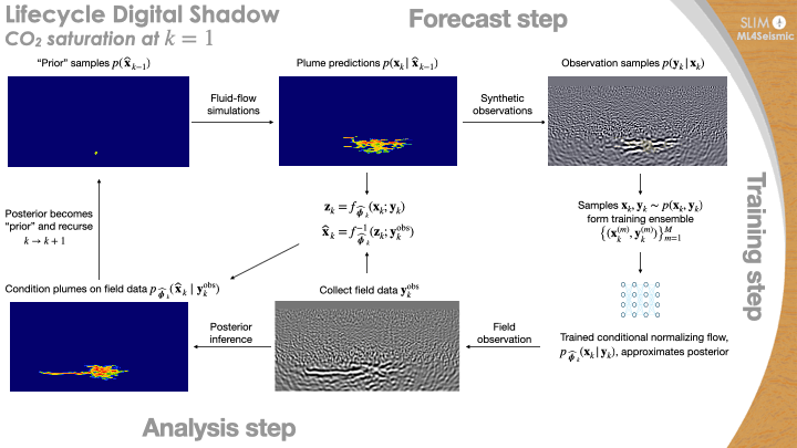
In collaboration with professor Edmond Chow and with support from the National Sciences Foundation, we have started work on the development of an uncertainty-aware “Digital Twin” for seismic monitoring of GCS. This Digital Twin extends our work on Bayesian Inference with (conditional) Normalizing Flows (NFs) described under Machine Learning. NFs are deep generative networks capable of approximating (conditional) probability distributions from samples generated from an invertible mapping from a latent distribution to a data distribution.

Given this ability to train NFs to approximate the conditional posterior distribution of the state of CO₂ plume, the proposed approach, outlined in Animation 2, works as follows: Suppose at some timestep we know how to generate samples from the probability distribution for the CO₂ plume conditioned on observed time-lapse data for the current state. Given these samples, we prepare the neural network for the next timestep by producing samples for the state of the CO₂ plume at that timestep via in silico simulations that capture our current understanding of the CO₂ dynamics. By coupling these time-advanced CO₂ plumes to simulated synthetic time-lapse seismic data, training pairs (state of CO₂ plume and seismic data) are created to update the conditional NF, which learns by example. With the updated NF, samples from the updated probability distribution can be drawn when the new time-lapse field data arrives at the next timestep. By following this procedure recursively, knowledge captured by the NF—i.e. the posterior distribution for the state of the CO₂ plume given the observed time-lapse data—remains current throughout CO₂ injection projects. During the Training Phase, the NF inside the Digital Twin is trained to approximate the posterior distribution for the next time-lapse timestep. Samples for the state of the CO₂ plume conditioned by the observed time-lapse field data are computed during the Inference Phase.

The design of our Digital Twin overlaps with five out of nine featured motives in a recent paper on Simulation Intelligence (Lavin et al. 2021)—(i) surrogate modeling of CO₂ dynamics; (ii) stochastic programming to generate sealed and leaking CO₂ plumes; (iii) simulation-based inference to approximate the posterior distribution of CO₂ conditioned by observed seismic data; (iv) differentiable programming to couple neural network surrogates with wave simulations and their hand-derived sensitivities; (v) machine programming to automatically generate highly-optimized code from the mathematical abstractions of Devito—to carry out symbolic finite difference computations, JUDI—to carry out inversion with Devito in Julia; InvertibleNetworks—to build high-performance building blocks for invertible neural networks in the Julia programming language; and integration with machine learning via ChainRules.jl.

Animation2Uncertainty-aware digital twin for geological carbon storage.

Figure 8 illustrates the “lifecycle” of our envisioned Digital Shadow for the first timestep, k = 1. A Digital Shadow corresponds to a Digital Twin but misses the ability to make decisions and optimize operations.

Figure 8: Life cycle of the recurrent Digital Shadow at timestep k = 1. Starting with the initial randomly chosen CO₂ saturation, a sample from the joint distribution,y_k ∼ p(x_k, y_k), is simulated during the *Forecast step*, consisting of fluid-flow and observation simulations. Samples from the joint distribution form a simulated training ensemble, {(x_k^(m), y_k^(m))}_m = 1^M, consisting of M training pairs that are to train the Ccondtional Normalizing Flow, which approximates the posterior. After training, the predicted plume is conditioned on the field data, y_k^* during the *Analysis step*, producing a samples from the CO₂ plume posterior distribution. These samples are used as samples for the “prior” at the next timestep.

References

Avseth, Per, Tapan Mukerji, and Gary Mavko. 2010. Quantitative Seismic Interpretation: Applying Rock Physics Tools to Reduce Interpretation Risk. Cambridge university press.

Chadwick, Andy, Gareth Williams, Nicolas Delepine, Vincent Clochard, Karine Labat, Susan Sturton, Maike-L Buddensiek, et al. 2010. “Quantitative Analysis of Time-Lapse Seismic Monitoring Data at the Sleipner CO 2 Storage Operation.” The Leading Edge 29 (2): 170–77.

Cranmer, Kyle, Johann Brehmer, and Gilles Louppe. 2020. “The Frontier of Simulation-Based Inference.” Proceedings of the National Academy of Sciences 117 (48): 30055–62.

Grady II, Thomas J, Rishi Khan, Mathias Louboutin, Ziyi Yin, Philipp A Witte, Ranveer Chandra, Russell J Hewett, and Felix J Herrmann. 2022. “Towards Large-Scale Learned Solvers for Parametric PDEs with Model-Parallel Fourier Neural Operators.” arXiv Preprint arXiv:2204.01205.

He, Kaiming, Xiangyu Zhang, Shaoqing Ren, and Jian Sun. 2016. “Deep Residual Learning for Image Recognition.” In Proceedings of the IEEE Conference on Computer Vision and Pattern Recognition, 770–78.

Jones, CE, JA Edgar, JI Selvage, and H Crook. 2012. “Building Complex Synthetic Models to Evaluate Acquisition Geometries and Velocity Inversion Technologies.” In 74th EAGE Conference and Exhibition Incorporating EUROPEC 2012, cp–293. European Association of Geoscientists & Engineers.

Klimentos, Theodoros. 1991. “The Effects of Porosity-Permeability-Clay Content on the Velocity of Compressional Waves.” Geophysics 56 (12): 1930–39.

Kragh, ED, and Phil Christie. 2002. “Seismic Repeatability, Normalized Rms, and Predictability.” The Leading Edge 21 (7): 640–47.

Lavin, Alexander, Hector Zenil, Brooks Paige, David Krakauer, Justin Gottschlich, Tim Mattson, Anima Anandkumar, et al. 2021. “Simulation Intelligence: Towards a New Generation of Scientific Methods.” arXiv Preprint arXiv:2112.03235.

Li, Dongzhuo, Kailai Xu, Jerry M Harris, and Eric Darve. 2020. “Coupled Time-Lapse Full-Waveform Inversion for Subsurface Flow Problems Using Intrusive Automatic Differentiation.” Water Resources Research 56 (8): e2019WR027032.

Li, Zongyi, Nikola Kovachki, Kamyar Azizzadenesheli, Burigede Liu, Kaushik Bhattacharya, Andrew Stuart, and Anima Anandkumar. 2020. “Fourier Neural Operator for Parametric Partial Differential Equations.” https://arxiv.org/abs/2010.08895.

Liu, Ze, Yutong Lin, Yue Cao, Han Hu, Yixuan Wei, Zheng Zhang, Stephen Lin, and Baining Guo. 2021. “Swin Transformer: Hierarchical Vision Transformer Using Shifted Windows.” In Proceedings of the IEEE/CVF International Conference on Computer Vision, 10012–22.

Lumley, David E. 2001. “Time-Lapse Seismic Reservoir Monitoring.” Geophysics 66 (1): 50–53.

Oghenekohwo, Felix. 2017. “Economic Time-Lapse Seismic Acquisition and Imaging—Reaping the Benefits of Randomized Sampling with Distributed Compressive Sensing.” PhD thesis, Vancouver: The University of British Columbia. https://slim.gatech.edu/Publications/Public/Thesis/2017/oghenekohwo2017THetl/oghenekohwo2017THetl.pdf.

Oghenekohwo, Felix, and Felix J. Herrmann. 2017. “Improved Time-Lapse Data Repeatability with Randomized Sampling and Distributed Compressive Sensing.” https://doi.org/10.3997/2214-4609.201701389.

Oghenekohwo, Felix, Haneet Wason, Ernie Esser, and Felix J. Herrmann. 2017. “Low-Cost Time-Lapse Seismic with Distributed Compressive Sensing-Part 1: Exploiting Common Information Among the Vintages.” Geophysics 82 (3): P1–13. https://doi.org/10.1190/geo2016-0076.1.

Ringrose, Philip. 2020. How to Store CO2 Underground: Insights from Early-Mover CCS Projects. Springer. https://link.springer.com/book/10.1007/978-3-030-33113-9.

Ringrose, Philip S, Anne-Kari Furre, Stuart MV Gilfillan, Samuel Krevor, Martin Landrø, Rory Leslie, Tip Meckel, Bamshad Nazarian, and Adeel Zahid. 2021. “Storage of Carbon Dioxide in Saline Aquifers: Physicochemical Processes, Key Constraints, and Scale-up Potential.” Annual Review of Chemical and Biomolecular Engineering 12: 471–94.

Rockström, Johan, Owen Gaffney, Joeri Rogelj, Malte Meinshausen, Nebojsa Nakicenovic, and Hans Joachim Schellnhuber. 2017. “A Roadmap for Rapid Decarbonization.” Science 355 (6331): 1269–71.

Simonyan, Karen, and Andrew Zisserman. 2014. “Very Deep Convolutional Networks for Large-Scale Image Recognition.” arXiv Preprint arXiv:1409.1556.

Vaswani, Ashish, Noam Shazeer, Niki Parmar, Jakob Uszkoreit, Llion Jones, Aidan N Gomez, Łukasz Kaiser, and Illia Polosukhin. 2017. “Attention Is All You Need.” Advances in Neural Information Processing Systems 30.

Wason, Haneet, Felix Oghenekohwo, and Felix J. Herrmann. 2017. “Low-Cost Time-Lapse Seismic with Distributed Compressive Sensing-Part 2: Impact on Repeatability.” Geophysics 82 (3): P15–30. https://doi.org/10.1190/geo2016-0252.1.

Wei, Lei, Yue Tian, Chang Li, Shauna Oppert, and Gilles Hennenfent. 2018. “Improve 4D Seismic Interpretability with Joint Sparsity Recovery.” In SEG Technical Program Expanded Abstracts 2018, 5338–42. Society of Exploration Geophysicists.

Witte, Philipp A., Mathias Louboutin, Fabio Luporini, Gerard J. Gorman, and Felix J. Herrmann. 2019. “Compressive Least-Squares Migration with on-the-Fly Fourier Transforms.” Geophysics 84 (5): R655–72. https://doi.org/10.1190/geo2018-0490.1.

Yang, Mengmeng, Zhilong Fang, Philipp A. Witte, and Felix J. Herrmann. 2020. “Time-Domain Sparsity Promoting Least-Squares Reverse Time Migration with Source Estimation.” Geophysical Prospecting 68 (9): 2697–2711. https://doi.org/10.1111/1365-2478.13021.

Yin, Wotao, Stanley Osher, Donald Goldfarb, and Jerome Darbon. 2008. “Bregman Iterative Algorithms for ∖Ell_1-Minimization with Applications to Compressed Sensing.” SIAM Journal on Imaging Sciences 1 (1): 143–68.

Yin, Ziyi, Mathias Louboutin, and Felix J. Herrmann. 2021. “Compressive Time-Lapse Seismic Monitoring of Carbon Storage and Sequestration with the Joint Recovery Model.” https://doi.org/10.1190/segam2021-3569087.1.

Zhou, Bolei, Aditya Khosla, Agata Lapedriza, Aude Oliva, and Antonio Torralba. 2016. “Learning Deep Features for Discriminative Localization.” In Proceedings of the IEEE Conference on Computer Vision and Pattern Recognition, 2921–29.

Seismic Laboratory for Imaging and Modeling