Simply denoise: wavefield reconstruction via jittered undersampling

Acknowledgments

G.H. thanks Ken Bube, Ramesh Neelamani, Warren Ross, Beatrice Vedel, and Ozgur Yilmaz for constructive discussions about this research. D.J. Verschuur and Chevron Energy Technology Company are gratefully thanked for the synthetic and real datasets, respectively. The authors thank the authors of CurveLab (www.curvelet.org) and the authors of SPGL1 (www.cs.ubc.ca/labs/scl/spgl1) for making their codes available. This paper was prepared with Madagascar, a reproducible research package (rsf.sourceforge.net). This work was in part financially supported by NSERC Discovery Grant 22R81254 and CRD Grant DNOISE 334810-05 of F.J.H. and was carried out as part of the SINBAD project with support, secured through ITF, from the following organizations: BG Group, BP, Chevron, ExxonMobil, and Shell.

We also appreciate the valuable comments and suggestions from the two reviewers and two associate editors.

Appendix A

append

[app:jit]Jittered undersampling For the convenience of the reader, we re-derive the result originally introduced by Leneman (1966) that leads to equation 6.

Jittered sampling locations $\,r_n$ are given by

$$r_n = n\gamma+\varepsilon_n \quad n = -\infty,\ldots,\infty$$ (10)

The continuous random variables $\,\varepsilon_n$ are independent and identically distributed (iid) according to a probability density function (pdf) p on $[-\zeta/2,\zeta/2]$ . The corresponding sampling operator $s$ is given by

$$s(r) = \sum_{n=-\infty}^{\infty}\delta(r-r_n).$$ (11)

Computing the Fourier transform of the previous expression yields

$$\hat{s}(f) = \frac{1}{\gamma}\sum_{n=-\infty}^{\infty}\delta\left(f-\frac{n}{\gamma}\right) ^{-i2\pi f\varepsilon_n}$$ (12)

which implies that

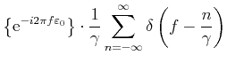$$\left\{\hat{s}(f)\right\} = \left\{\text{e}^{-i2\pi f\varepsilon_0}\right\}\cdot\frac{1}{\gamma}\sum_{n=-\infty}^{\infty}\delta\left(f-\frac{n}{\gamma}\right)$$ (13)

since the variables $\,\varepsilon_n$ are iid. By definition, the expected value of $\,$e$^{-i2\pi f\varepsilon_0}\,$ is given by

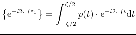$$\left\{\text{e}^{-i2\pi f\varepsilon_0}\right\} = \int_{-\zeta/2}^{\zeta/2}p(t)\cdot\text{e}^{-i2\pi ft}\text{d}t$$ (14)

which is the Fourier transform of the pdf of $\,\varepsilon_0$ . Hence,

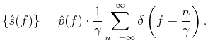$$\left\{\hat{s}(f)\right\} = \hat{p}(f)\cdot\frac{1}{\gamma}\sum_{n=-\infty}^{\infty}\delta\left(f-\frac{n}{\gamma}\right).$$ (15)

Finally, for a pdf that is continuous uniform on $[-\zeta/2,\zeta/2]$ , the expected spectrum of the sampling operator is

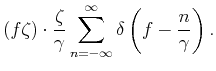$$\left\{\hat{s}(f)\right\} = \left(f\zeta\right)\cdot\frac{\zeta}{\gamma}\sum_{n=-\infty}^{\infty}\delta\left(f-\frac{n}{\gamma}\right).$$ (16)

This result leads us to equation 6 since the columns of $\tensor{A}^H\tensor{A}$ are circular-shifted versions of the Fourier transform of the discrete jittered sampling vector, i.e., diag$(\tensor{R}^H\tensor{R})$ .

Simply denoise: wavefield reconstruction via jittered undersampling