Simply denoise: wavefield reconstruction via jittered undersampling

Fourier-domain artifacts of the jittered grid

When $\tensor{R}$ describes a jittered undersampling scheme according to a discrete uniform distribution, the stochastic expectation E$\{\cdot\}$ of the first column $\ensuremath{\mathbf{a}}$ of the circulant matrix $\tensor{A}^H\tensor{A}$ is given by

$$\left\{\ensuremath{\mathbf{a}}[k]\right\} \approx \left\{ \begin{... ...=\frac{\gamma+1}{2},\ldots,\gamma-1\\ 0 & \text{otherwise}, \end{array} \right.$$ (6)

where sinc$(\cdot)$ is the normalized sinc function defined as sinc$(x) \; {\buildrel\rm def\over=}\; \sin(\pi x)/\pi x$ .

reg,sinc,res
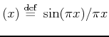
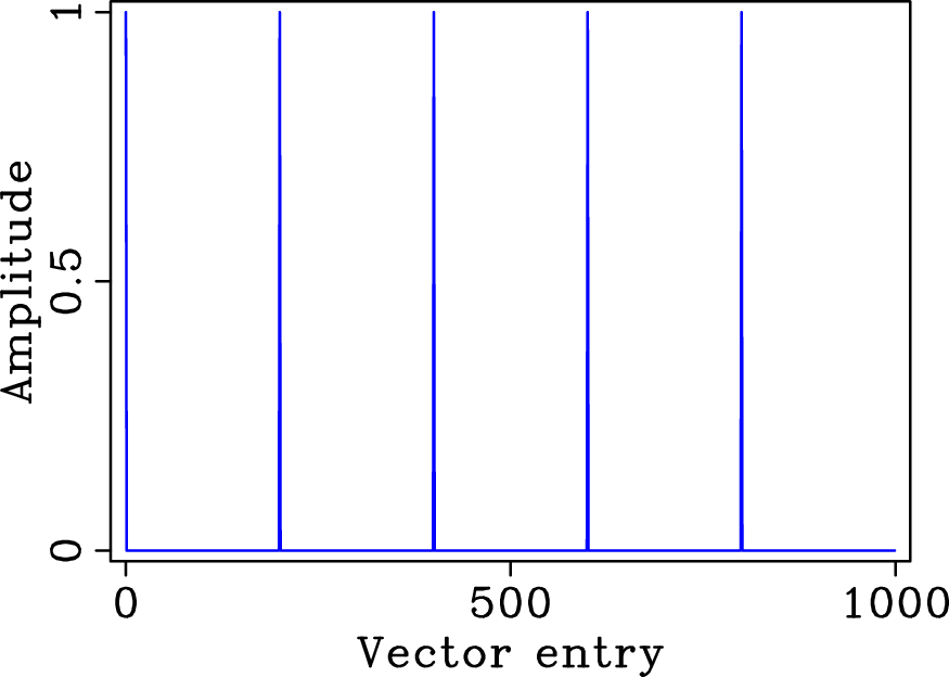
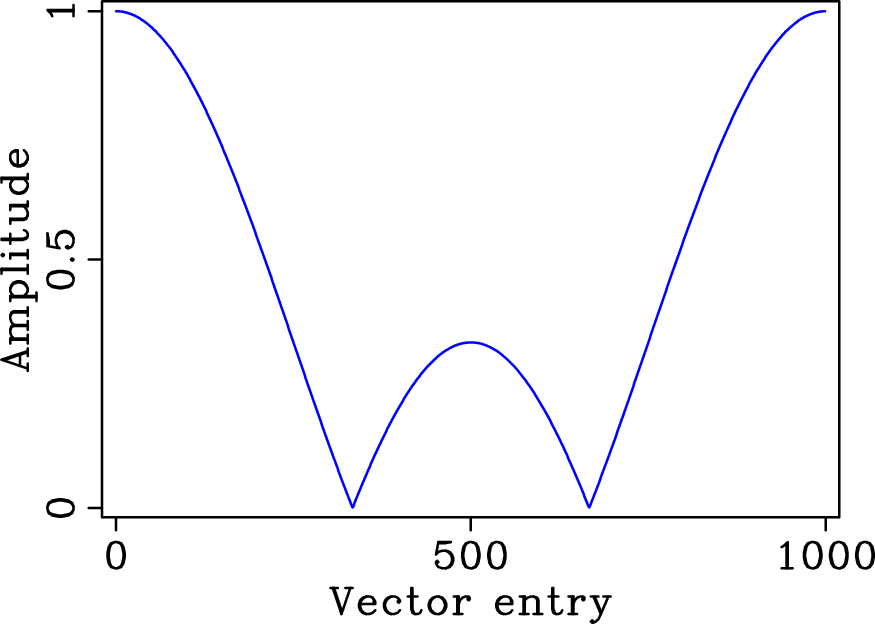
Figure 4. Amplitude spectrum of (a) a five-fold ($\gamma =5$ ) regular undersampling vector, (b) a three-sample wide uniform distribution ($\xi =3$ ), and (c) the resulting jittered undersampling vector. The first half of the vectors contains the positive frequencies starting with zero, the second half contains the negative frequencies in decreasing order.

The above expression corresponds to an elementwise multiplication of the periodic Fourier spectrum of the discrete regular sampling vector with a sinc function. This sinc function follows from the Fourier transform of the probability density function for the perturbation with respect to a point of the regularly decimated grid.

In Figure 4 the amplitudes for this Fourier-domain multiplication are plotted for jittered undersampling with $\gamma =5$ and $\xi =3$ , i.e., on average four-out-of-five samples are missing for a jitter that includes the decimated grid point, one sample on the right and one sample on the left (cf. Figure 3, second row).

Equation 6 is a special case of the result for jittered undersampling according to an arbitrary distribution introduced by Leneman (1966) and further detailed in Appendix A. Because these results were originally derived for the continuous case, the above expression is approximate. In practice, however, this formula proves to be accurate, an observation corroborated by numerical results presented below. Consider the following cases for a fixed undersampling factor $\gamma$ .

Simply denoise: wavefield reconstruction via jittered undersampling