|
|
|
|
Simply denoise: wavefield reconstruction via jittered undersampling |
For this purpose, we define the sparsifying transform
![]() as
the Fourier transform
as
the Fourier transform
![]() , i.e.,
, i.e.,
![]() , and generate a vector
, and generate a vector
![]() with
with
![]() nonzero entries and of length
nonzero entries and of length ![]() . The nonzero entries of
. The nonzero entries of
![]() are distributed at random with random signs and
amplitudes. The to-be-recovered signal
are distributed at random with random signs and
amplitudes. The to-be-recovered signal
![]() is given by
is given by
![]() and the observations
and the observations
![]() are obtained by undersampling
are obtained by undersampling
![]() regularly,
randomly according to a discrete uniform distribution, or
optimally-jittered, i.e.,
regularly,
randomly according to a discrete uniform distribution, or
optimally-jittered, i.e.,
![]() . Finally, the estimated
spectrum
. Finally, the estimated
spectrum
![]() of
of
![]() is obtained by solving
equation 3 with the Spectral Projected Gradient for
is obtained by solving
equation 3 with the Spectral Projected Gradient for
![]() solver (SPGL1 - van den Berg and Friedlander, 2007). Keep in mind that the
number
solver (SPGL1 - van den Berg and Friedlander, 2007). Keep in mind that the
number ![]() of nonzero entries of
of nonzero entries of
![]() is not known a priori.
Each experiment is repeated 100 times for the different undersampling
schemes and for varying undersampling factors
is not known a priori.
Each experiment is repeated 100 times for the different undersampling
schemes and for varying undersampling factors ![]() , ranging from 2
to 6. The reconstruction error is the number of entries at which the
estimated representation
, ranging from 2
to 6. The reconstruction error is the number of entries at which the
estimated representation
![]() and the true
representation
and the true
representation
![]() of
of
![]() in the Fourier domain
disagree by more than
in the Fourier domain
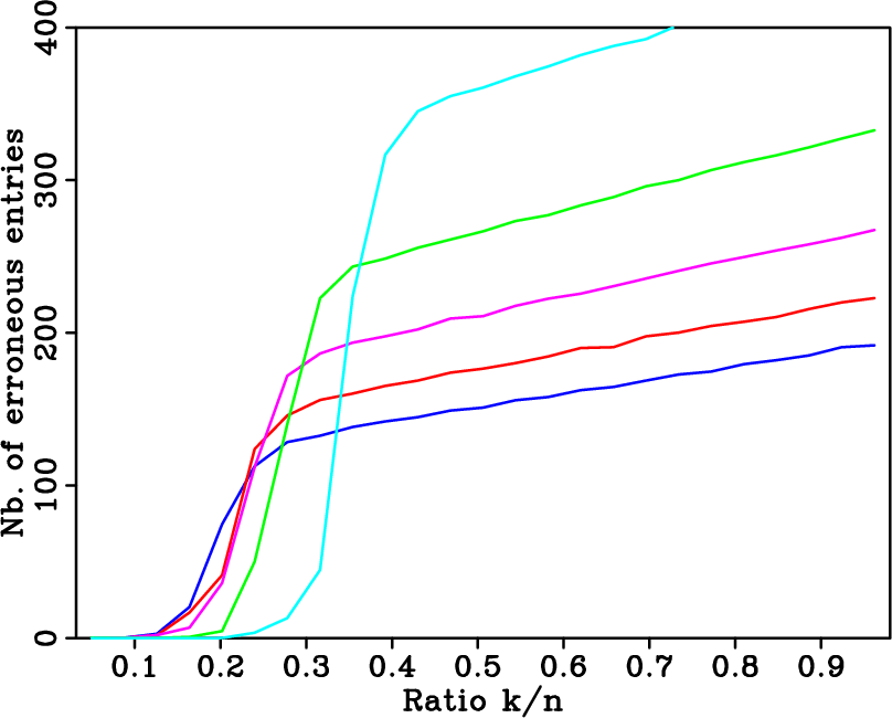
disagree by more than ![]() . This error accounts for both false
positives and false negatives. The averaged results for the different
experiments are summarized in Figures 6(a),
6(b), and 6(c), which
correspond to regular, random, and optimally-jittered undersampling,
respectively. The horizontal axes in these plots represent the
relative underdeterminedness of the system, i.e., the ratio of the
number
. This error accounts for both false
positives and false negatives. The averaged results for the different
experiments are summarized in Figures 6(a),
6(b), and 6(c), which
correspond to regular, random, and optimally-jittered undersampling,
respectively. The horizontal axes in these plots represent the
relative underdeterminedness of the system, i.e., the ratio of the
number ![]() of nonzero entries in
of nonzero entries in
![]() to the number
to the number ![]() of
acquired data points. The vertical axes represent the average
reconstruction error. The different curves represents the different
undersampling factors. In each plot, the curves from top to bottom
correspond to
of
acquired data points. The vertical axes represent the average
reconstruction error. The different curves represents the different
undersampling factors. In each plot, the curves from top to bottom
correspond to
![]() .
.
Figure 6(a) shows that, regardless of the
undersampling factor, there is no range of relative
underdeterminedness for which
![]() can accurately be
recovered from a regular undersampling of
can accurately be
recovered from a regular undersampling of
![]() . Sparsity is
not enough to discriminate the signal components from the spectral
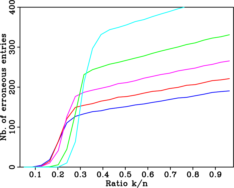
leakage. The situation is completely different in Figures
6(b) and 6(c) for the random
and optimally-jittered sampling. In this case, one can observed that
exact recovery is possible for
. Sparsity is
not enough to discriminate the signal components from the spectral
leakage. The situation is completely different in Figures
6(b) and 6(c) for the random
and optimally-jittered sampling. In this case, one can observed that
exact recovery is possible for
![]() . The main purpose
of these plots is to qualitatively show the transition from successful
to failed recovery. The quantitative interpretation for these
diagrams to the right of the transition is less well understood but
also observed in phase diagrams published in the literature
(Donoho et al., 2006). A possible explanation for the observed
behavior of the error lies in the nonlinear behavior of the solvers
and on an error not measured in the
. The main purpose
of these plots is to qualitatively show the transition from successful
to failed recovery. The quantitative interpretation for these
diagrams to the right of the transition is less well understood but
also observed in phase diagrams published in the literature
(Donoho et al., 2006). A possible explanation for the observed
behavior of the error lies in the nonlinear behavior of the solvers
and on an error not measured in the ![]() sense.
sense.
The key observations from these experiments are threefold. First, it
is possible, under specific conditions, to exactly recover by
sparsity-promoting inversion the original spectrum
![]() of
of
![]() from (very) few data points. Secondly,
optimally-jittered undersampling behaves like random undersampling
according to a discrete uniform distribution. For practical purposes,
the former can thus be seen as equivalent to the latter. Thirdly, not
all undersampling schemes for a given undersampling factor are
comparable from a CS perspective. Regular undersampling is the most
challenging. Random and optimally-jittered undersamplings according to
a discrete uniform distribution are among the most favorable. In
particular, if the signal is sufficiently sparse, these schemes lead
to a reconstruction as good as dense regular sampling.
Translated to the reconstruction of seismic wavefields, these results
hint at a new nonlinear sampling theory based on a sparsifying
transform for complex seismic data, e.g., the curvelet transform, and
a coarse random sampling scheme that creates favorable recovery
conditions for that transform, e.g., optimally-jittered undersampling.
from (very) few data points. Secondly,
optimally-jittered undersampling behaves like random undersampling
according to a discrete uniform distribution. For practical purposes,
the former can thus be seen as equivalent to the latter. Thirdly, not
all undersampling schemes for a given undersampling factor are
comparable from a CS perspective. Regular undersampling is the most
challenging. Random and optimally-jittered undersamplings according to
a discrete uniform distribution are among the most favorable. In
particular, if the signal is sufficiently sparse, these schemes lead
to a reconstruction as good as dense regular sampling.
Translated to the reconstruction of seismic wavefields, these results
hint at a new nonlinear sampling theory based on a sparsifying
transform for complex seismic data, e.g., the curvelet transform, and
a coarse random sampling scheme that creates favorable recovery
conditions for that transform, e.g., optimally-jittered undersampling.

|
|---|
|
phasediagREG,phasediagIRREG,phasediagJIT1
Figure 6. Averaged recovery errors for a |
|
|
|
|
|
|
Simply denoise: wavefield reconstruction via jittered undersampling |