|
|
|
|
Simply denoise: wavefield reconstruction via jittered undersampling |
To keep the derivation of our jittered undersampling scheme succinct,
the undersampling factor, ![]() , is taken to be odd, i.e.,
, is taken to be odd, i.e.,
![]() We also assume that the size
We also assume that the size ![]() of the
interpolation grid is a multiple of
of the
interpolation grid is a multiple of ![]() so that the number of
acquired data points
so that the number of
acquired data points
![]() is an integer. For these choices,
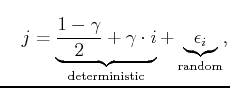
the jittered-sampled data points are given by
is an integer. For these choices,
the jittered-sampled data points are given by
|
|---|
|
schemjit
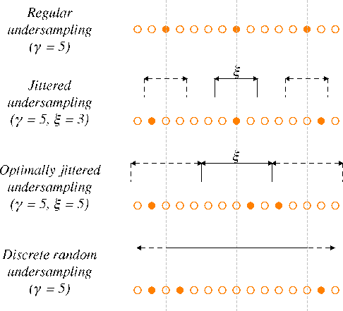
Figure 3. Schematic comparison between different undersampling schemes. The circles define the fine grid on which the original signal is alias-free. The solid circles represent the actual sampling points for the different undersampling schemes. The jitter parameter |
|
|
In Figure 3, schematic illustrations are included for
samplings with increasing randomness. The fine grid of open circles
denotes the interpolation grid on which the model
![]() is
defined. The solid circles correspond to the coarse sampling
locations. These illustrations show that for jittered undersampling,
the maximum gap size can not exceed
is
defined. The solid circles correspond to the coarse sampling
locations. These illustrations show that for jittered undersampling,
the maximum gap size can not exceed
![]() data points. For regular
undersampling, all the gaps are of size
data points. For regular
undersampling, all the gaps are of size ![]() and for random
undersampling according to a discrete uniform distribution, the
maximum gap size is
and for random
undersampling according to a discrete uniform distribution, the
maximum gap size is ![]() . Remember that the number of samples is the
same for each of these undersampling schemes.
. Remember that the number of samples is the
same for each of these undersampling schemes.
As mentioned earlier, recovery with localized transforms depends on both the maximum gap size and a sufficient sampling randomness to break the coherent aliases. In the next section, we show how the value of the jitter parameter controls these two aspects in our undersampling scheme.
|
|
|
|
Simply denoise: wavefield reconstruction via jittered undersampling |