Time-domain Wavefield Reconstruction Inversion in a TTI medium

Abstract

We introduce a generalization of time-domain wavefield reconstruction inversion to anisotropic acoustic modeling. Wavefield reconstruction inversion has been extensively researched in recent years for its ability to mitigate cycle skipping. The original method was formulated in the frequency domain with acoustic isotropic physics. However, frequency-domain modeling requires sophisticated iterative solvers that are difficult to scale to industrial-size problems and more realistic physical assumptions, such as tilted transverse isotropy, object of this study. The work presented here is based on a recently proposed dual formulation of wavefield reconstruction inversion, which allows time-domain propagator that are suitable to both large scales and more accurate physics.

Introduction

Wave-equation based seismic imaging has become increasingly popular due to its ability to produce detailed and accurate subsurface models. In recent years, however, the limitations of Full Waveform Inversion (FWI) have been widely acknowledged due to the cycle skipping issue that arises with bandlimited data and lack of long offsets (thus low frequencies). Simple geological settings, such as shallow water sedimentary areas, have showcased the benefits of FWI, but more challenging problems involve complex subsurface structures such as salt bodies with strong anisotropy, which requires extensive manual intervention for a consistently successful application. To address these limitations, extended formulation have driven some of the most recent research in seismic imaging. These methods rely on extra variables, usually a wavefield (Tristan van Leeuwen and Herrmann, 2013; T. van Leeuwen and Herrmann, 2013) as in Wavefield Reconstruction Inversion (WRI) or time-space dependent source (Huang et al., 2018; C. Wang et al., 2016) in the extended source method. Extra unknowns are designed to absorb inaccuracies in the initial background model by relaxing the physics, while additional constraints ensure that this relaxation is ultimately driven to a physically consistent scenario. One of the main challenges associated with extended formulations is the necessity to solve for an augmented least-squares system that, in the frequency domain, is only feasible for small to mid-size problems with simple representations of the physics or for industry-sized problems but of limited type of acquisition geometries (Bas Peters and Herrmann, 2019). Conventional time-domain propagators, on the contrary, do not share the same limitations.

This work is based on the time-domain formulation of WRI (Rizzuti et al., 2019) which relies on conventional time-stepping (M. Louboutin et al., 2019; Symes, 2015). Therefore, it straightforwardly allows the adoption of a more accurate representation of the physics. In this paper, we focus on the transverse tilted isotropic (TTI) wave-equation (Y. Zhang et al., 2011; Bube et al., 2016; Louboutin et al., 2018). The inclusion of anisotropic effects are indeed crucial for the inversion of field data. Note that frequency-domain methods do not enable TTI anisotropy in full generality, with the exception of the limited vertical transverse anisotropy (VTI) (Aghamiry et al., 2019). Regardless, VTI WRI still relies on iterative solvers for the augmented system, and is therefore unfeasible for realistic sizes.

In this paper, we highlight the benefits of the time-domain WRI method (B. Peters et al., 2014; Tristan van Leeuwen and Herrmann, 2013; Rizzuti et al., 2019) for TTI inversion and we demonstrate that TWRI can compensate for inaccuracies in the anisotropic parameters in addition to compensating for a poor initial model. We briefly introduce the dual formulation of WRI, then present two examples that demonstrate that TTI WRI is feasible and more robust than FWI with respect to modeling faulty assumptions.

Methodology

In previous work (Rizzuti et al., 2019), we introduced the dual formulation of WRI, which only requires conventional forward and adjoint propagators in time domain and do not need the solution of the extended wave equation. Time-domain WRI starts from the constrained least-squares problem: \[ \begin{equation} \min_{\bm,\bu}\dfrac{1}{2}\norm{\bq-\A\bu}^2\quad\mathrm{s.t.}\quad\norm{\bd-\R\bu}\leq\varepsilon, \label{eq:denoise} \end{equation} \] where \(\bm\) represents the physical properties of interest and \(\bu\) is the associated wavefield. The data is denoted by \(\bd\) and \(\bq\) is the (known) source term. The wave equation is denominated by \(\A\) and \(\R\) is receiver-restriction operator. We then derive the reduced Lagrangian associated with Eq. \(\ref{eq:denoise}\) (c.f (Rockafellar, 1970; Rizzuti et al., 2020)) to obtain the TWRI objective function: \[ \begin{equation} \begin{split} & \max_{\by}\min_{\bm}\LWRId(\bm,\by),\\ & \LWRId(\bm,\by)=-\dfrac{1}{2}\norm{\F^{\ast}\by}^2+\<\by,\br\>-\varepsilon\norm{\by}, \end{split} \label{lagr_red} \end{equation} \]

where the forward operator \(\F=\R\A^{-1}\) is the forward modeling operator, and \(\br=\bd - \F \bq\) the data residual for the model \(\bm\). This dual problem has two unknowns, parameters \(\bm\) (squared slowness), and variables \(\by\)(having the same size of data). One of the advantages of the formulation in Eq. \(\ref{lagr_red}\) is that, unlike conventional WRI, the additional variable is of a manageable size (compared to wavefields). To update the model \(\bm\), we calculate the derivative: \[ \begin{equation} \nabla_{\bm}\LWRId=-J[\bm,\bq+\F^{\ast}\by]^{\ast}\by, \label{lagr_red_gradm} \end{equation} \] where \(J\) is the conventional FWI Jacobian operator for an extended source \(\bq+\F^{\ast}\by\). It is straightforward to extend the previous acoustic implementation to the Transverse Tilted Isotropic case (TTI, Y. Zhang et al., 2011; Duveneck and Bakker, 2011; Louboutin et al., 2018), just by simply replacing \(\F\) with its TTI counterpart.

Previous work have demonstrated that TWRI behaves more robustly than FWI with respect to local minimum issues in the purely acoustic case. Here we illustrate that the edge of WRI over FWI still holds for TTI and, more importantly, when the assumed physics do not match with the collected data.

Numerical experiments

These two examples aim to elucidate two main advantages of TWRI. First, since we use a time-domain formulation that only necessitates the implementation of standard forward and adjoint propagators, we are able to implement TTI TWRI by simply replacing the acoustic time-stepper with an anisotropic version thereof. Moreover, thanks to Devito (M. Louboutin et al., 2019; Luporini et al., 2018) and JUDI(Witte et al., 2019), these propagators are implemented in a simple high-level way and benefit from its highly efficient just-in-time compiler. Finally, we show that TTI TWRI mitigates cycle skipping either with true anisotropy parameters and a kinematically inaccurate initial model, or with inaccurate anisotropic parameters and a fair initial model. Finally, we verify a known secondary advantage of WRI that is its robustness to inaccurate water layer velocity and ocean bottom position.

We concentrate on three increasingly difficult settings over these examples:

1. Invert the TTI data with a TTI wave-equation and assuming the true anisotropy parameters are known.
2. Invert the TTI data with a TTI wave-equation with error introduced in the anisotropic parameters.
3. Invert the TTI data with an acoustic wave-equation.

The first two cases demonstrate the TWRI mitigates the sensitivity to cycle skipping associated with both the velocity and anisotropy errors. The third case demonstrates that TWRI can compensate for a numerical representation of the physics that does not correspond to the physics of the observed data.

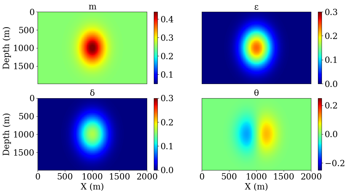
Gaussian lens

This first example follows (Huang et al., 2018) with a 2D singularity model with a constant initial model. This model in known to be cycle skipped and demonstrate the capability of TWRI to obtain a better update direction than conventional FWI. To further highlight the robustness with respect to the Thomsen parameters(Thomsen, 1986), we fix these to zero and compute the gradient. This parameterization shows that TWRI can compensate for anisotropy errors for the computation of the gradient with respect to the squared slowness.

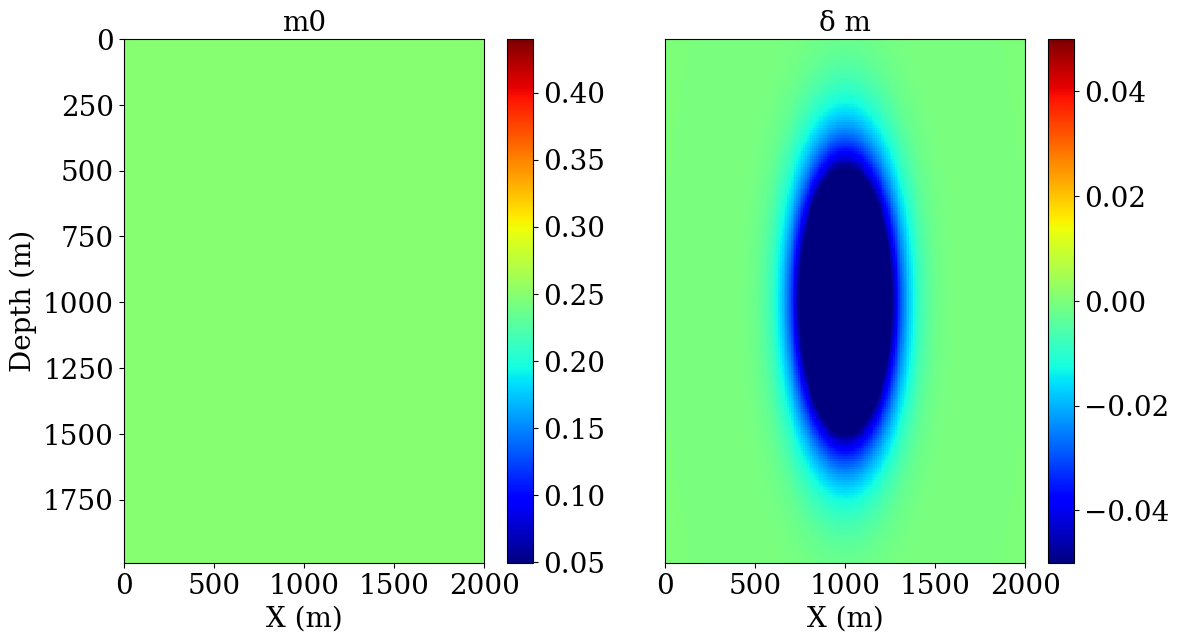
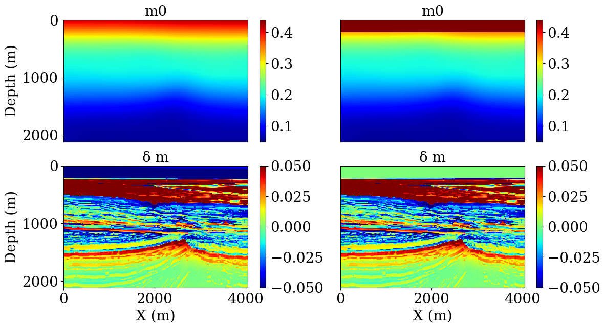
We show the initial model (constant velocity) and true perturbation in Figure 2, and we expect to see the gradient update to have the same sign as the true perturbation in Figure 2.

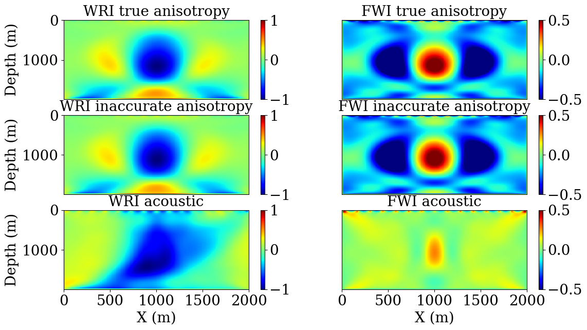
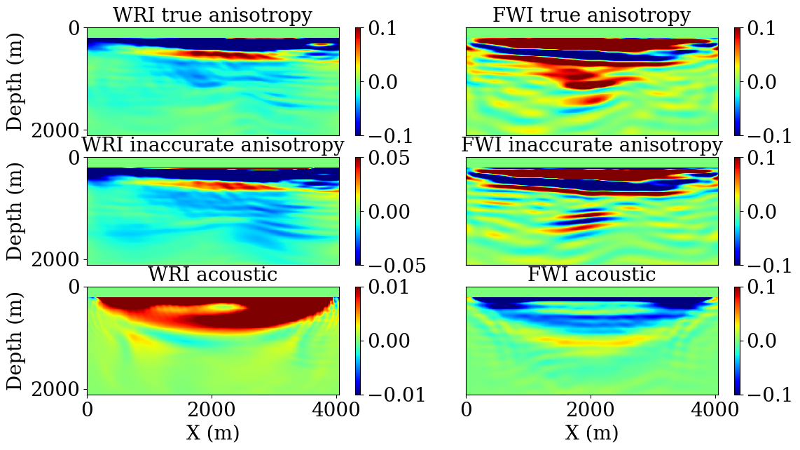
The gradient obtained with each of the three cases are displayed on Figure 3. We first see that, as expected from previous work, FWI does not produce a good update direction as the sign is flipped compared to the true perturbation (FIgure 2) and optimizations algorithms will not converge to a good solution. On the other hand, we can see that in all three cases, the update direction obtained with TWRI is consistent with the true perturbation and will lead to a good model reconstruction. One interesting observation is that TWRI correctly handles the errors in the anisotropy, including for the complete absence of anisotropy in the modeling kernel. Such result is encouraging in light of more realistic examples.

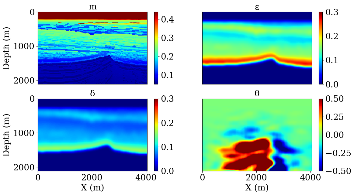
BG Compass

The second example involves the BG Compass model. The Thomsen parameters are synthesized from the velocity model, while dip angles are inferred from the orientation of the layers. We show the TTI parameters in Figure 4. This model is notoriously difficult due to the velocity kick back (situated at around the one kilometer depth on Figure 4) that prevents turning waves from traveling back to the surface.

This experiment is divided in two settings. On one hand, we assume the water velocity and depth of the water layer to be known and look at the first update computed with TWRI and FWI. In the second case, we do not assume any knowledge of the water layer, that is known to be delignated by WRI in the acoustic case, and once again look at the first FWI and TWWRI update. These two initial models and the true perturbation associated with it are on Figure 5, and a good update is expected to correlate with the true perturbation well while a cycle skipped update would have the wrong sign in most areas in particular for the velocity kick-back part.

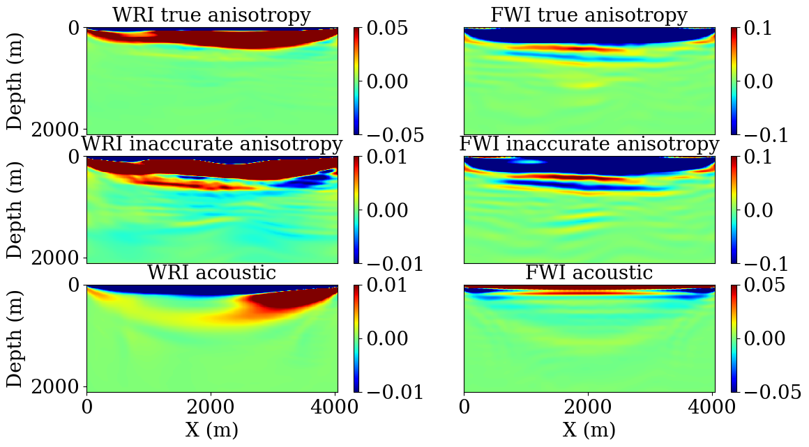
The results obtained with the correct water velocity are shown in Figure 6. Similarly to the previous example, TWRI succeeds to capture most of the features of the true perturbation while FWI displays major differences. The most difficult part of the model to image is the middle section around 1 km depth. The velocity kick-back makes the inversion very difficult as the turning wave are diving deeper into the model rather than going back up towards the receivers. We can see that TWRI perfectly captures this velocity kick back while FWI only succeeds to match partially the shallower part of the model.

In the second part of this experiment, the results obtained with the incorrect water velocity are shown on Figure 6. As expected from previous results (B. Peters et al., 2014), TWRI provides a correct update direction in the water layer while still featuring the attributes necessary for inversion such as the previously mentioned velocity kick-back.

These examples and related software can be found at TTIWRI in our reproducibility repository https://github.com/slimgroup/Software.SEG2020.

Discussion & conclusions

In this work, we presented an application of TWRI to a realistic inversion scenario, by including TTI physics. Because our work is based on time-domain modeling, we can leverage on state of the art anisotropic propagators. The extension to anisotropy is not trivial in the frequency domain due to the current limitations of iterative solvers for large-scale, coupled PDEs. We experimented that TWRI not only produces more qualitative results that conventional FWI when data and modeling physics matches, but also fairs better with respect to modeling inaccuracies, e.g. when the inverted data presents anisotropic effects but an acoustic medium is postulated. While these preliminary results are encouraging, future work will focus on a more thorough validation of TWRI for TTI media and applications to 3D examples.

References

Aghamiry, H., Gholami, A., and Operto, S., 2019, Multi-parameter aDMM-based wavefield reconstruction inversion in vTI acoustic media:, 2019, 1–5. doi:https://doi.org/10.3997/2214-4609.201900871
Bube, K., Washbourne, J., Ergas, R., and Nemeth, T., 2016, Self-adjoint, energy-conserving second-order pseudoacoustic systems for vTI and tTI media for reverse time migration and full-waveform inversion: In SEG technical program expanded abstracts 2016 (pp. 1110–1114). doi:10.1190/segam2016-13878451.1
Duveneck, E., and Bakker, P. M., 2011, Stable p-wave modeling for reverse-time migration in tilted tI media: GEOPHYSICS, 76, S65–S75. doi:10.1190/1.3533964
Huang, G., Nammour, R., and Symes, W. W., 2018, Volume source-based extended waveform inversion: Geophysics, 83, R369–R387.
Leeuwen, T. van, and Herrmann, F. J., 2013, Mitigating local minima in full-waveform inversion by expanding the search space: Geophysical Journal International, 195, 661–667. doi:10.1093/gji/ggt258
Leeuwen, T. van, and Herrmann, F. J., 2013, Mitigating local minima in full-waveform inversion by expanding the search space: Geophys. J. Int., 195, 661–667. doi:10.1093/gji/ggt258
Louboutin, M., Lange, M., Luporini, F., Kukreja, N., Witte, P. A., Herrmann, F. J., … Gorman, G. J., 2019, Devito (v3.1.0): An embedded domain-specific language for finite differences and geophysical exploration: Geoscientific Model Development, 12, 1165–1187. doi:10.5194/gmd-12-1165-2019
Louboutin, M., Witte, P. A., and Herrmann, F. J., 2018, Effects of wrong adjoints for rTM in tTI media: SEG technical program expanded abstracts. doi:10.1190/segam2018-2996274.1
Luporini, F., Lange, M., Louboutin, M., Kukreja, N., Hückelheim, J., Yount, C., … Herrmann, F. J., 2018, Architecture and performance of devito, a system for automated stencil computation: CoRR, abs/1807.03032. Retrieved from http://arxiv.org/abs/1807.03032
Peters, B., and Herrmann, F. J., 2019, A numerical solver for least-squares sub-problems in 3D wavefield reconstruction inversion and related problem formulations: SEG technical program expanded abstracts. doi:10.1190/segam2019-3216638.1
Peters, B., Herrmann, F., and Leeuwen, T. van, 2014, Wave-equation based inversion with the penalty method - adjoint-state versus wavefield-reconstruction inversion:, 2014, 1–5. doi:https://doi.org/10.3997/2214-4609.20140704
Rizzuti, G., Louboutin, M., Wang, R., and Herrmann, F. J., 2020, Time-domain wavefield reconstruction inversion for large-scale seismics:. Retrieved from https://slim.gatech.edu/Publications/Public/Conferences/EAGE/2020/rizzuti2020EAGEtwri/rizzuti2020EAGEtwri.html
Rizzuti, G., Louboutin, M., Wang, R., Daskalakis, E., and Herrmann, F. J., 2019, A dual formulation for time-domain wavefield reconstruction inversion: SEG technical program expanded abstracts. doi:10.1190/segam2019-3216760.1
Rockafellar, R. T., 1970, Convex analysis: Princeton University Press.
Symes, W. W., 2015, IWAVE structure and basic use cases: THE RICE INVERSION PROJECT, 85. Retrieved from http://www.trip.caam.rice.edu/reports/2014/book.pdf#page=89
Thomsen, L., 1986, Weak elastic anisotropy: Geophysics, 51, 1964–1966.
Wang, C., Yingst, D., Farmer, P., and Leveille, J., 2016, Full-waveform inversion with the reconstructed wavefield method: In SEG technical program expanded abstracts 2016 (pp. 1237–1241). Society of Exploration Geophysicists.
Witte, P. A., Louboutin, M., Kukreja, N., Luporini, F., Lange, M., Gorman, G. J., and Herrmann, F. J., 2019, A large-scale framework for symbolic implementations of seismic inversion algorithms in julia: GEOPHYSICS, 84, F57–F71. doi:10.1190/geo2018-0174.1
Zhang, Y., Zhang, H., and Zhang, G., 2011, A stable tTI reverse time migration and its implementation: GEOPHYSICS, 76, WA3–WA11. doi:10.1190/1.3554411