Time-domain wavefield reconstruction inversion for large-scale seismics

Introduction

Wave-equation-based seismic inversion techniques are nowadays mature for 3D large-scale deployment, and are becoming a valuable tool in seismic exploration. State-of-the-art time-stepping solvers ensure feasibility on the hardware available to the oil-and-gas industry (and even to a wider audience thanks to cloud computing). Classical inversion methods, however, suffer from local minimum stagnation, which has limited their scope so far. Recently, model extension methods, such as wavefield reconstruction inversion, have demonstrated remarkable results in mitigating this issue. This class of methods, however, leverages on added complexity, which can seriously curtail their application to large problems. For example, wavefield reconstruction inversion (WRI) requires the solution of augmented version of the wave equation, which cannot be trivially solved in a time-marching fashion, and is, therefore, not readily suited to 3D. Here, we propose a dual (Lagrangian) reformulation of WRI, which naturally lends itself to conventional time-domain solvers and large-scale applications, while retaining the robustness of the original method with respect to local minima.

Theory

Classical inversion

Modern seismic inversion is cast as an optimization problem endowed with partial differential equation (PDE) constraints. Given a suitable discretization of the physical quantities of interest, and the algebraic operators that govern their mutual relationship, the problem is expressed as: \[ \begin{equation} \min_{\bm,\bu}\dfrac{1}{2}\norm{\bd-\R\bu}^2\quad\mathrm{subject\ to}\quad\A\bu=\bq. \label{eqinvprobgen} \end{equation} \] Data \(\bd\in\Real^{\Nt\times\Nr\times\Ns}\) is recorded in time at \(\Nr\) receiver locations for different \(\Ns\) source positions. When appropriate, after a temporal Fourier transform, \(\bd\in\Compl^{\Nf\times\Nr\times\Ns}\) for different \(\Nf\) frequencies. The variable \(\bu\in\Real^{N\times\Nt\times\Ns}\) (or \(\bu\in\Compl^{N\times\Nf\times\Ns}\), in frequency domain) represents a wavefield, discretized on an \(N\)-dimensional space (\(N\) being the number of grid points of the discretized physical domain). The wave equation is encoded by the linear system \(\A\bu=\bq\). Note that \(\A\) is parameterized by the physical quantity \(\bm\) that will indicate, throughout this paper, the acoustic squared slowness. The right-hand side \(\bq\) is typically a point source. In Equation \(\eqref{eqinvprobgen}\), data is compared to the interpolated values of \(\bu\), via the operator \(R\).

For industrial-scale 3D problems, the grid size is \(N=O(n^3)\) (in big O notation) with \(n\sim1000\) grid points. With conservative source/receiver acquisition coverage, \(\Nr=O(n)\), \(\Ns=O(n)\). Furthermore, when time-domain methods with explicit time-marching schemes are applied, \(\Nt=O(n)\), due to solver stability conditions. In the frequency domain, for full-bandwidth imaging, we still formally need \(\Nf=O(n)\), although the complexity constants can be relaxed considerably with respect to the time domain. In this large-scale regime, the need for affordable memory and time complexity poses extraordinary challenges. For instance, the storage for the wavefields \(\bu\) grows as \(O(n^5)\), and cannot be attained for each source/time sample at once. Time-complexity is determined by the computation of the solutions of the wave equation. Frequency domain methods are less favorable to 3D, as this amounts to solving or solutions of a large, sparse, non-definite linear system, and do not scale as efficiently as explicit time-domain approaches, which currently remain the only practical option.

Despite these challenges, many techniques such as full-waveform inversion (FWI) (Virieux and Operto, 2009) are now viable for industrial-size problems, especially when the simulated physics is simple (e.g., acoustics). FWI enforces PDE constraints directly as \(\bu=\A^{-1}\bq\): \[ \begin{equation} \min_{\bm}\frac{1}{2}||\bd-F(\bm)\,\bq||^2,\quad F(\bm)=R\,A(\bm)^{-1}, \label{eqFWI} \end{equation} \] thus avoiding the need for simultaneously storing wavefields for each source. However, the FWI objective function is multimodal and is not easily tackled by local-search optimization. Traditionally, considerable problem-specific intervention was required to consistently ensure its success.

Wavefield reconstruction inversion (WRI)

Recently, model extension methods (W. W. Symes, 2008), based on adding slack unknowns to the original problem, have proven their robustness to local minima, but are usually hampered by the computational costs associated to working in higher dimension. For example, WRI (Leeuwen and Herrmann, 2013) aims to the reconstruction of both model parameters \(\bm\) and wavefields \(\bu\): \[ \begin{equation} \min_{\bm,\bu}\J(\bm,\bu),\quad\J(\bm,\bu)=\dfrac{1}{2}\norm{\bd-\R\bu}^2+\dfrac{\phantom{^2}\lambda^2}{2}\norm{\bq-\A\bu}^2. \label{eqWRI} \end{equation} \] A reduced objective \(\bar{\J}(\bm)=\min_{\bu}\J(\bm,\bu)=\J(\bm,\bub)\) can be obtained by variable projection, where \(\bub\) is the solution of the augmented wave equation \[ \begin{equation} \begin{split} \begin{pmatrix} \R\\ \lambda\A\\ \end{pmatrix}\bub= \begin{pmatrix} \bd\\ \lambda\bq\\ \end{pmatrix}\, . \end{split} \label{eqWRIweq} \end{equation} \] Solving for \(\bub\) for each source avoids the need for simultaneous storage (similarly to FWI), but time-marching schemes are not available for Equation \(\eqref{eqWRIweq}\) (contrary to FWI). Therefore this method cannot be trivially extended to 3D.

A dual formulation for time-domain WRI (TWRI*)

In this section, we formulate our proposal for a scalable time-domain version of WRI, here referred to as TWRI* (where the notation \(^*\) refers to the following dual approach). The starting point is the denoising reformulation of Equation \(\eqref{eqWRIweq}\): \[ \begin{equation} \min_{\bm,\bu}\dfrac{1}{2}\norm{\bq-\A\bu}^2\quad\mathrm{s.t.}\quad\norm{\bd-\R\bu}\leq\varepsilon, \label{eqDenoise} \end{equation} \] for a known noise level \(\varepsilon\). The Lagrangian associated to Equation \(\eqref{eqDenoise}\) takes the form \[ \begin{equation} \L(\bm,\bu,\by)=\dfrac{1}{2}\norm{\bq-\A\bu}^2+\<\by,\bd-\R\bu\>-\varepsilon\norm{\by}, \label{eqLagr} \end{equation} \] where the multipliers \(\by\) belong to a linear space with the same dimension as data. Similarly to WRI, the wavefield variables \(\bu\) can be eliminated from Equation \(\eqref{eqLagr}\) by applying variable projection: \[ \begin{equation} \A\bub=\bq+\F^*\by, \label{eqTWRIwav} \end{equation} \] yielding \[ \begin{equation} \L(\bm,\by)=-\dfrac{1}{2}\norm{\F^*\by}^2+\<\by,\br\>-\varepsilon\norm{\by}, \label{eqLagr_red} \end{equation} \] where the forward operator \(\F\) was defined in Equation \(\eqref{eqFWI}\), and \(\br\) is the data residual for the model \(\bm\). Furthermore: \[ \begin{equation} \nabla_{\bm}\L=-J[\bm,\bq+\F^*\by]^*\by,\quad\nabla_{\by}\L=\bd-\F(\bq+\F^*\by)-\varepsilon\by/\norm{\by}. \label{eqLagrGrad} \end{equation} \] Here, \(J[\bm,\bfb]\) is the Jacobian of the mapping \(\bm\mapsto\F\bfb\) (and \(J[\bm,\bfb]^*\) its adjoint).

The evaluation of the Lagrangian \(\L\) and its gradients only requires solutions of a conventional wave equation. The additional multipliers \(\by\) can be stored in memory whenever joint (\(\bm\), \(\by\)) optimization is carried out.

Note that, for a fixed \(\bm\), the optimal \(\bar{\by}\) must solve the non-linear system: \[ \begin{equation} \varepsilon\dfrac{\bar{\by}}{\norm{\bar{\by}}}+\F\F^*\bar{\by}=\br, \label{eqWRIdual_yopt} \end{equation} \] An iterative solution of this equation will likely result in an expensive scheme. As a result, we propose—similarly to Wang et al. (2016) — a computationally cheap approximation corresponding to the scaled data residual, \(\bar{\by}\approx\tilde{\by}=\alpha\br\), albeit for an unknown scalar \(\alpha\) (calculated in closed form by maximizing the Lagrangian in Equation \(\eqref{eqLagr_red}\)). This substitution leads to a reduced objective \(\tilde{\L}=\L(\bm,\tilde{\by})\) function of only \(\bm\). A rigorous computation of the gradient with respect to \(\bm\) yields \[ \begin{equation} \nabla_{\bm}\tilde{\L} = \nabla_{\bm}\L(\bm,\tilde{\by})-\alpha J[\bm,\bq]^*\nabla_{\by}\L(\bm,\tilde{\by}). \label{eqWRIgradcorr} \end{equation} \] Compared to FWI, the resulting formulation requires twice as many solutions of the wave equation, per objective evaluation (2 vs 1 solves) or gradient computation (4 vs 2 solves). Despite the increased cost, this still compares favorably to conventional WRI, since we avoid the need to solve for an augmented wave equation. On the other hand, we gained the robustness of conventional WRI against local minima, as demonstrated with numerical examples.

Examples

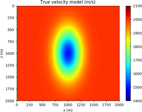
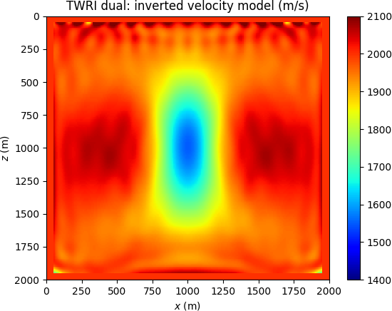
Low-velocity lens

We consider the Gaussian lens model presented in (Huang et al., 2018), here depicted in Figure (1a). The challenge is to image a low-velocity anomaly of Gaussian shape from transmission data, knowing an homogeneous background model. Synthetic data are generated with a Ricker source wavelet of \(10\) Hz peak frequency (corresponding to a spatial wavelength of \(200\) m). The FWI result (1b) clearly represents a spurious local minimum, while TWRI* (1c) is converging to the correct model.

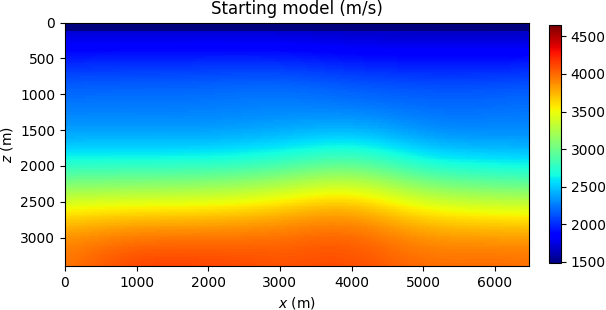
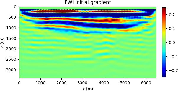
BG Compass

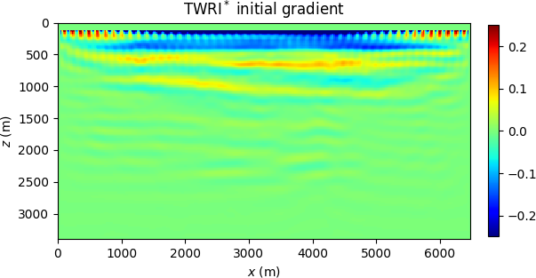
For the BG Compass model depicted in Figure (2) (see also Peters et al. (2014)), sources and receivers are placed at the surface, and synthetic data is generated with a \(10\) Hz Ricker wavelet. Further preprocessing ensures that the frequency components below \(5\) Hz are removed. In Figure (3), we compare the \(5.5\) Hz components of the initial gradients of FWI and TWRI*, which illustrates the difficulty of FWI to correctly update the water layer. The final result for TWRI* is shown in Figure (4).

Conclusions

We introduced a scalable dual reformulation of WRI, TWRI*, based on a model extension by means of dual data multipliers (as opposed to wavefield variables in the original WRI). Since dual variables have the same dimension of data, a joint optimization over model and dual parameters might be devised. In this paper, however, we eliminate these extra unknowns by choosing a filtered version of the data residual, as a cheap estimate. We demonstrated, through numerical experimentation, that the resulting scheme remains relatively robust against local minima. Its objective function can be evaluated and differentiated by using conventional time domain solvers (with a computational cost corresponding to roughly twice what is required for FWI), and is therefore amenable for 3D applications.

Related material

Acknowledgments

This work has been implemented in Julia and leverages on the Devito framework for seismic modeling, which allows automatic generation of highly-optimized finite-difference C code, given only a symbolic representation of the wave equation (M. Louboutin et al., 2019). From Julia, we interface to Devito through the JUDI package (P. A. Witte et al., 2019).