Reliable amortized variational inference with physics-based latent distribution correction

Introduction

Inverse problems involve the estimation of an unknown quantity based on noisy indirect observations. The problem is typically solved by minimizing the difference between observed and predicted data, where predicted data can be computed by modeling the underlying data generation process through a forward operator. Due to the presence of noise in the data, forward modeling errors, and the inherent nullspace of the forward operator, minimization of the data misfit alone negatively impacts the quality of the obtained solution (Aster et al., 2018). Casting inverse problems into a probabilistic Bayesian framework allows for a more comprehensive description of their solution, where instead of finding one single solution, a distribution of solutions to the inverse problem—known as the posterior distribution—is obtained whose samples are consistent with the observed data (Tarantola, 2005). The posterior distribution can be sampled to extract statistical information that allows for quantification of uncertainty, i.e., assessing the variability among the possible solutions to the inverse problem.

Uncertainty qualification and Bayesian inference in inverse problems often require high-dimensional posterior distribution sampling, for instance through the use of Markov chain Monte Carlo (MCMC, Robert and Casella, 2004; Martin et al., 2012; Fang et al., 2018; Siahkoohi et al., 2022c). Because of their sequential nature, MCMC sampling methods require a large number of sampling steps to perform accurate Bayesian inference (Gelman et al., 2013), which reduces their applicability to large-scale problems due to the high-dimensionality of the unknown and costs associated with the forward operator (Curtis and Lomax, 2001; Welling and Teh, 2011; Martin et al., 2012; Fang et al., 2018; Herrmann et al., 2019; Z. Zhao and Sen, 2019; Kotsi et al., 2020; Siahkoohi et al., 2020a, 2020b). As an alternative, variational inference methods (M. I. Jordan et al., 1999; Wainwright and Jordan, 2008; Rezende and Mohamed, 2015; Q. Liu and Wang, 2016; Rizzuti et al., 2020; X. Zhang and Curtis, 2020; Tölle et al., 2021; D. Li et al., 2021; D. Li, 2022) approximate the posterior distribution with a surrogate and easy-to-sample distribution. By means of this approximation, sampling is turned into an optimization problem, in which the parameters of the surrogate distribution are tuned in order to minimize the divergence between the surrogate and posterior distributions. This surrogate distribution is then used for conducting Bayesian inference. While variational inference methods may have computational advantages over MCMC methods in high-dimensional inverse problems (Blei et al., 2017; X. Zhang et al., 2021), the resulting approximation to the posterior distribution is typically non-amortized, i.e., it is specific to the observed data used in solving the variational inference optimization problem. Thus, the variational inference optimization problem must be solved again for every new set of observations. Solving this optimization problem may require numerous iterations (Rizzuti et al., 2020; X. Zhang and Curtis, 2020), which may not be feasible in inverse problems with computationally costly forward operators, such as seismic imaging.

On the other hand, amortized variational inference (Kim et al., 2018; Baptista et al., 2020; Kruse et al., 2021; N. Kovachki et al., 2021; S. T. Radev et al., 2022; Siahkoohi et al., 2021, 2022b; Ren et al., 2021; Siahkoohi and Herrmann, 2021; Khorashadizadeh et al., 2022; Orozco et al., 2021; Taghvaei and Hosseini, 2022) reduces Bayesian inference computational costs by incurring an up-front optimization cost for finding a surrogate conditional distribution, typically parameterized by deep neural networks (Kruse et al., 2021), that approximate the posterior distribution across a family of observed data instead of being specific to a single observed dataset. This supervised learning problem involves maximization of the probability density function (PDF) of the surrogate conditional distribution over existing pairs model and data (S. T. Radev et al., 2022). Following optimization, samples from the posterior distribution for previously unseen data may be obtained by sampling the surrogate conditional distribution, which does not require further optimization or MCMC sampling. While drastically reducing the cost of Bayesian inference, amortized variational inference can only be used for inverse problems where a dataset of model and data pairs is available that sufficiently captures the underlying joint distribution. In reality, such an assumption is rarely true in geophysical applications due to the Earth’s strong heterogeneity across geological scenarios and our lack of access to its interior (Siahkoohi et al., 2021; Sun et al., 2021; P. Jin et al., 2022). Additionally, the accuracy of Bayesian inference with data-driven amortized variational inference methods degrades as the distribution of the data shifts with respect to pretraining data (Schmitt et al., 2021). Among these shifts are changes in the distribution of noise, the number of observed data in multi-source inverse problems, and the distribution of unknowns, in other words, the prior distribution.

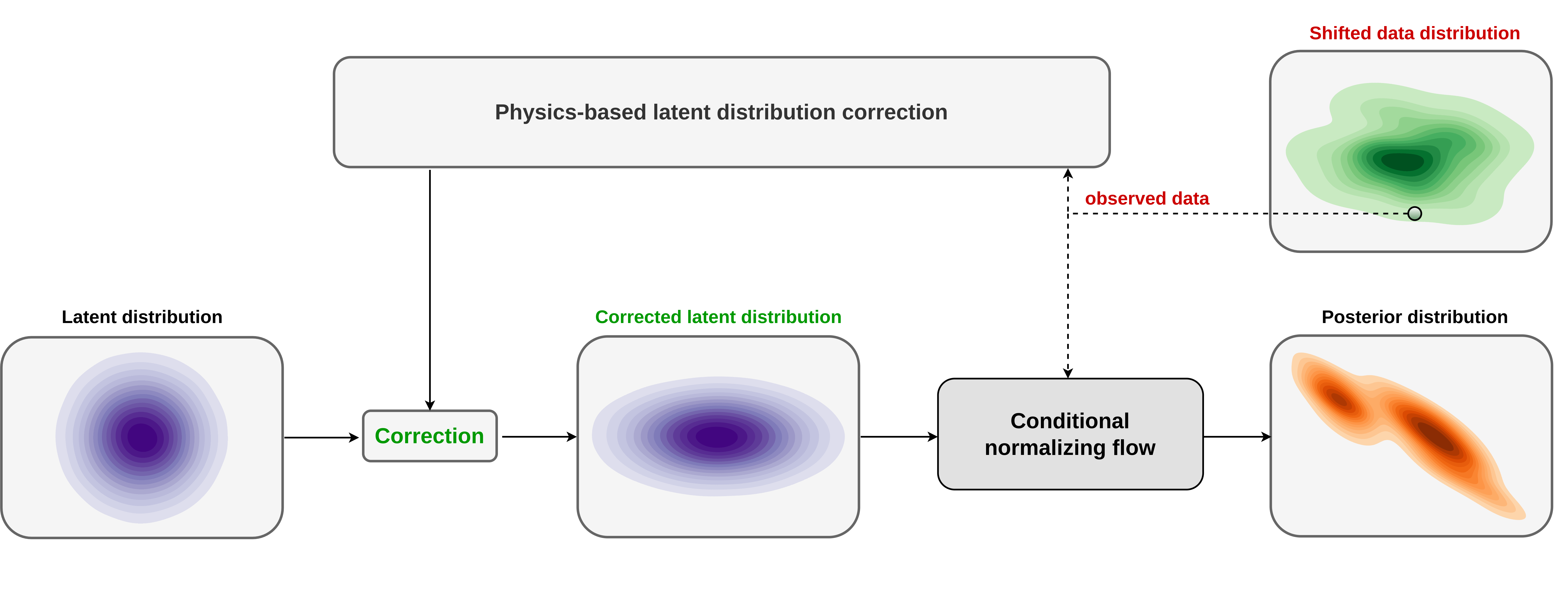
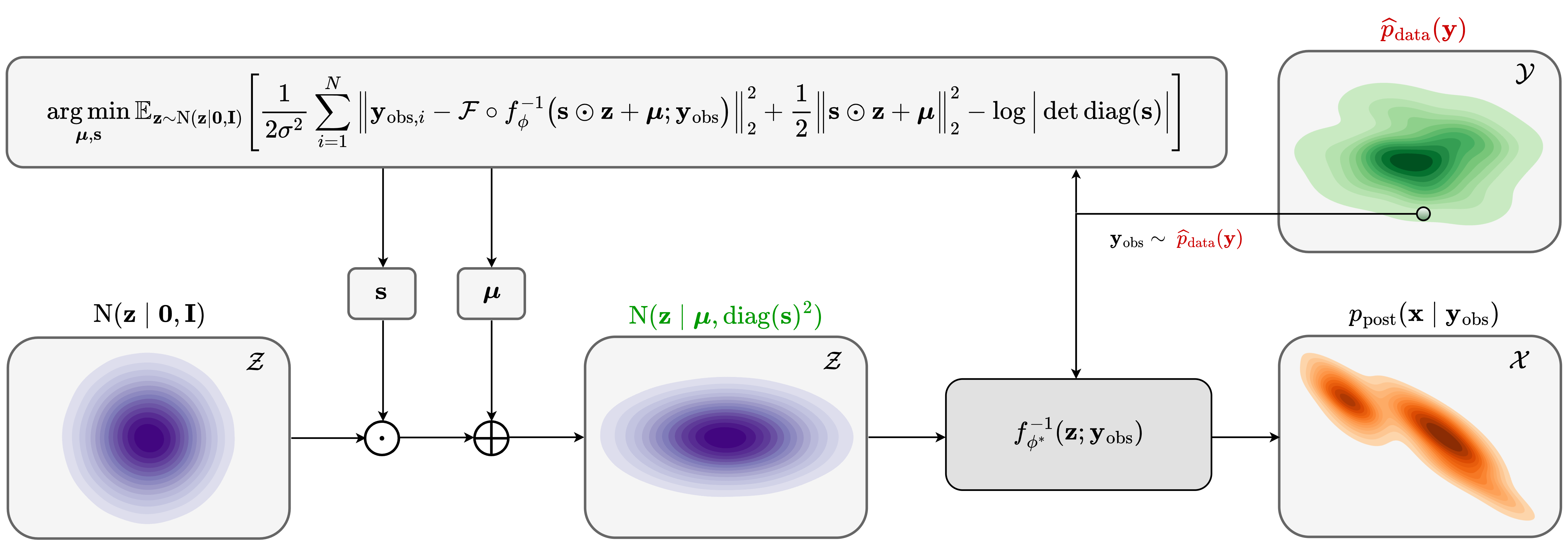
In this work, we leverage amortized variational inference to accelerate Bayesian inference while building resilience against data distribution shifts through an unsupervised, data-specific, a physics-based latent distribution correction method. During this process, the latent distribution of a normalizing-flow-based surrogate conditional distribution (Kruse et al., 2021) is corrected to minimize the Kullback-Leibler (KL) divergence between the predicted and true posterior distributions. The invertibility of the conditional normalizing flow—a family of invertible neural networks (Dinh et al., 2016)—guarantees the existence of a corrected latent distribution (Asim et al., 2020) that when “pushed forward” by the conditional normalization flow matches the posterior distribution. During pretraining, the conditional normalizing flow learns to Gaussianize the input model and data joint samples (Kruse et al., 2021), resulting in a standard Gaussian latent distribution. As a result, for slightly shifted data distributions, the conditional normalization flow can provide samples from the the posterior distribution given an “approximately Gaussian” latent distribution as input (Parno and Marzouk, 2018; Peherstorfer and Marzouk, 2019). Motivated by this, and to limit the costs of the latent distribution correction step, we learn a simple diagonal (elementwise) scaling and shift to the latent distribution through a physic-based objective that minimizes the KL divergence between the predicted and true posterior distributions. As with amortized variational inference, after latent distribution correction, we gain cheap access to corrected posterior samples. Besides offering computational advantages, our proposed method implicitly learns the prior distribution during conditional normalizing flow pretraining. As advocated in the literature (Bora et al., 2017; Asim et al., 2020) learned priors have the potential to better describe the prior information when compared to generic handcrafted priors that are chosen purely for their simplicity and applicability. A schematic representation of our proposed method is shown in Figure 1.

Related work

In the context of variational inference for inverse problems, Rizzuti et al. (2020), Andrle et al. (2021), Zhao et al. (2021), X. Zhang and Curtis (2021), and Zhao et al. (2022) proposed a non-amortized variational inference approach to approximate posterior distributions through the use of normalizing flows. These methods do not require training data, however they require choosing a prior distribution and repeated computationally expensive evaluation of the forward operator and the adjoint of its Jacobian. Therefore, the proposed methods may prove computationally expensive when applied to inverse problems involving computationally expensive forward operators. To speed up the convergence of non-amortized variational inference, Siahkoohi et al. (2021) introduces a normalizing-flow-based nonlinear preconditioning scheme. In this approach, a pretrained conditional normalizing flow capable of providing a low-fidelity approximation to the posterior distribution is used to warm-start the variational inference optimization procedure. In a related work, Kothari et al. (2021) partially address challenges associated with non-amortized variational inference by learning a normalizing-flow-based prior distribution in a learned low-dimensional space via an injective network. Additionally to learning a prior, this approach also allowed non-amortized variational inference in a lower dimensional space, which could potentially have computational benefits.

Alternatively, amortized variational inference was applied by Adler and Öktem (2018), Kruse et al. (2021), N. Kovachki et al. (2021), Siahkoohi and Herrmann (2021), and Khorashadizadeh et al. (2022) to further reduce the computational costs associated with Bayesian inference. These supervised methods learn an implicit prior distribution from training data and provide posterior samples for previously unseen data for a negligible cost due to the low cost of forward evaluation of neural networks. The success of such techniques hinges on having access to high-quality training data, including pairs of model and data that sufficiently capture the underlying model and data joint distribution. To address this limitation, Siahkoohi et al. (2021) take amortized variational inference a step further by proposing a two-stage multifidelity approach where during the first stage a conditional normalizing flow is trained in the context of amortized variational inference. To account for any potential shift in data distribution, the weights of this pretrained conditional normalizing flow are then further finetuned during an optional second stage of physics-based variational inference, which is customized for the specific imaging problem at hand. While limiting the risk of errors caused by shifts in the distribution of data, the second physics-based stage can be computationally expensive due to the high dimensionality of the weight space of conditional normalizing flows. Our work differs from the proposed method in Siahkoohi et al. (2021) in that we learn to correct the latent distribution of the conditional normalizing flow, which typically has a much smaller dimensionality (approximately \(\times 90\) in our case) than the dimension of the conditional normalizing flow weight space.

The work we present is principally motivated by Asim et al. (2020), which demonstrates that normalizing flows—due to their invertibility—can mitigate biases caused by shifts in the data distribution. This is achieved by reparameterizing the unknown by a pretrained normalizing flow with fixed weights while optimizing over the latent variable in order to fit the data. The reparameterization together with a Gaussian prior on the latent variable act as a regularization while the invertibility ensures the existence of a latent variable that fits the data. Asim et al. (2020) exploit this property using a normalizing flow that is pretrained to capture the prior distribution associated with an inverse problem. By computing the maximum-a-posterior estimate in the latent space, Asim et al. (2020), as well as D. Li (2022) and Orozco et al. (2021), limit biases originating from data distribution shifts while utilizing the prior knowledge of the normalizing flow. We extend this method by obtaining an approximation to the full posterior distribution of an inverse problem instead of a point estimate, e.g., maximum-a-posteriori.

Our work is also closely related to the non-amortized variational inference techniques presented by Whang et al. (2021) and Kothari et al. (2021), in which the latent distribution of a normalizing flow is altered in an unsupervised way in order to perform Bayesian inference. In contrast to our approach, these methods employ a pretrained normalizing flow that approximates the prior distribution. As a result, it is necessary to significantly alter the latent distribution in order to correct the pretrained normalizing flow to sample from the posterior distribution. In response, Whang et al. (2021) and Kothari et al. (2021) train a second normalizing flow aimed at learning a latent distribution that approximates the posterior distribution after passing through the pretrained normalizing flow. Our study, however, utilizes a conditional normalizing flow, which, before any corrections are applied, already approximates the posterior distribution. We argue that our approach requires a simpler correction in the latent space to mitigate biases caused by shifts in the data distribution. This is crucial when dealing with large-scale inverse problems with computationally expensive forward operators.

Main contributions

The main contribution of our work involves a variational inference formulation for solving probabilistic Bayesian inverse problems that leverages the benefits of data-driven learned posteriors whilst being informed by physics and data. The advantages of this formulation include

• Enhancing the solution quality of inverse problems by implicitly learning the prior distribution from the data;

• Reliably reducing the cost of uncertainty quantification and Bayesian inference; and

• Providing safeguards against data distribution shifts.

Outline

In the sections below, we first formulate multi-source inverse problems mathematically and cast them within a Bayesian framework. We then describe variational inference and examine how existing model and data pairs can be used to obtain an approximation to the posterior distribution that is amortized, i.e., the approximation holds over a distribution of data rather than a specific set of observations. We showcase amortized variational inference on a high-dimensional seismic imaging example in a controlled setting where we assume observed data during inference is drawn from the same distribution as training seismic data. As means to mitigate potential errors due to data distribution shifts, we introduce our proposed correction approach to amortized variational inference, which exploits the advantages of learned posteriors while reducing potential errors induced by certain data distribution shifts. Two linearized seismic imaging examples are presented, in which the distribution of the data (simulated via linearized Born modeling) is shifted by altering the forward model and the prior distribution. These numerical experiments are intended to demonstrate the ability of the proposed latent distribution correction method to correct for errors caused by shifts in the distribution of data. Finally, we verify our proposed Bayesian inference method by conducting posterior contraction experiments.

Theory

Our purpose is to present a technique for using deep neural networks to accelerate Bayesian inference for ill-posed inverse problems while ensuring that the inference is robust with respect to data distribution shifts through the use of physics. We begin with an introduction to Bayesian inverse problems and discuss variational inference (M. I. Jordan et al., 1999) as a probabilistic framework for solving Bayesian inverse problems.

Inverse problems

We are concerned with estimating an unknown multidimensional quantity \(\B{x}^{\ast} \in \mathcal{X}\), often referred to as the unknown model, given \(N\) noisy and indirect observed data (e.g, shot records in seismic imaging) \(\B{y} = \{\B{y}_i\}_{i=1}^N\) with \(\B{y}_i \in \mathcal{Y}\). Here \(\mathcal{X}\) and \(\mathcal{Y}\) denote the space of unknown models and data, respectively. The physical underlying data generation process is assumed to be encoded in forward modeling operators, \(\mathcal{F}_i:\mathcal{X} \rightarrow \mathcal{Y}\), which relates the unknown model to the observed data via the forward model \[ \begin{equation} \B{y}_i = \mathcal{F}_i(\B{x}^{\ast}) + \boldsymbol{\epsilon}_i, \quad i=1,\dots,N. \label{forward_model} \end{equation} \] In the above expression, \(\boldsymbol{\epsilon}_i\) is a vector of measurement noise, which might also include errors in the forward modeling operator. Solving ill-posed inverse problems is challenged by noise in the observed data, potential errors in the forward modeling operator, and the intrinsic nontrivial nullspace of the forward operator (Aster et al., 2018). These challenges can lead to non-unique solutions where different estimates of the unknown model may fit the observed data equally well. Under such conditions, the use of a single model estimate ignores the intrinsic variability within inverse problem solutions, which increases the risk of overfitting the data. Therefore, not only the process of estimating \(\B{x}^{\ast}\) from \(\B{y}\) requires regularization, but it also calls for a statistical inference framework that allows us to characterize the variability among the solutions by quantifying the solution uncertainty (Tarantola, 2005).

Bayesian inference for solving inverse problems

To systematically quantify the uncertainty, we cast the inverse problem into a Bayesian framework (Tarantola, 2005). In this framework, instead of having a single estimate of the unknown, the solution is characterized by a probability distribution over the solution space \(\mathcal{X}\) that is conditioned on data, namely the posterior distribution. This conditional distribution, denoted by \(p_{\text{post}} (\B{x} \mid \B{y})\), can according to the Bayes’ rule be written as follows: \[ \begin{equation} p_{\text{post}} (\B{x} \mid \B{y}) = \frac{p_{\text{like}} (\B{y} \mid \B{x})\, p_{\text{prior}} (\B{x})}{p_{\text{data}} (\B{y})}. \label{bayes_rule} \end{equation} \] which equivalently can be expressed as \[ \begin{equation} \begin{aligned} - \log p_{\text{post}} (\B{x} \mid \B{y}) & = - \sum_{i=1}^{N} \log p_{\text{like}} (\B{y}_i \mid \B{x} ) - \log p_{\text{prior}} (\B{x}) + \log p_{\text{data}} (\B{y}) \\ & = \frac{1}{2 \sigma^2} \sum_{i=1}^{N} \big \| \B{y}_i-\mathcal{F}_i(\B{x}) \big\|_2^2 - \log p_{\text{prior}} (\B{x}) + \text{const}, \end{aligned} \label{bayes_rule_log} \end{equation} \] in case the observed data (\(\B{y}_i\)) are independent conditioned on the unknown model \(\B{x}\). In equations \(\ref{bayes_rule}\) and \(\ref{bayes_rule_log}\), the likelihood function \(p_{\text{like}} (\B{y} \mid \B{x})\) quantifies how well the predicted data fits the observed data given the PDF of the noise distribution. For simplicity, we assume the distribution of the noise is a zero-mean Gaussian distribution with covariance \(\sigma^2 \B{I}\) but other choices can be incorporated. The prior distribution \(p_{\text{prior}} (\B{x})\) encodes prior beliefs on the unknown quantity, which can also be interpreted as a regularizer for the inverse problem. Finally, \(p_{\text{data}} (\B{y})\) denotes the data PDF, which is a normalization constant that is independent of \(\B{x}\).

Acquiring statistical information regarding the posterior distribution requires access to samples from the posterior distribution. Sampling the posterior distribution, commonly achieved via MCMC (Robert and Casella, 2004) or variational inference techniques (M. I. Jordan et al., 1999), is computationally costly in high-dimensional inverse problems due to the costs associated with many needed evaluations of the forward operator (Malinverno and Briggs, 2004; Tarantola, 2005; Malinverno and Parker, 2006; Martin et al., 2012; Blei et al., 2017; Ray et al., 2017; Fang et al., 2018; G. K. Stuart et al., 2019; Z. Zhao and Sen, 2019; Kotsi et al., 2020; X. Zhang et al., 2021). For multi-source inverse problem the costs are especially high as evaluating the likelihood function involves \(N\) forward operator evaluations (equation \(\ref{bayes_rule_log}\)). Stochastic gradient Langevin dynamics (SGLD; Welling and Teh, 2011; C. Li et al., 2016; Siahkoohi et al., 2022c) alleviates the need to evaluate the likelihood for all the \(N\) forward operators by allowing for stochastic approximations to the likelihood, i.e., evaluating the likelihood over randomly selected indices \(i \in \{1, \ldots, N \}\). While SGLD can provably provide accurate posterior samples with more favorable computational costs (Welling and Teh, 2011), due to the sequential nature of MCMC methods, SGLD still requires numerous iterations to fully traverse the probability space (Gelman et al., 2013), which is computationally challenging in large-scale multi-source inverse problems. In the next section, we introduce variational inference as an alternative Bayesian inference method that has the potential to scale better than MCMC-methods in inverse problems with costly forward operators (Blei et al., 2017; X. Zhang et al., 2021).

Variational inference

As an alternative to MCMC-based methods, variational inference methods (M. I. Jordan et al., 1999) reduce the problem of sampling from the posterior distribution \(p_{\text{post}} (\B{x} \mid \B{y})\) to an optimization problem. The optimization problem involves approximating the posterior PDF via the PDF of a tractable surrogate distribution \(p_{\phi} (\B{x})\) with parameters \(\Bs{\phi}\) by minimizing a divergence (read “distance”) between \(p_{\phi} (\B{x})\) and \(p_{\text{post}}(\B{x} \mid \B{y})\) with respect to surrogate distribution parameters \(\Bs{\phi}\). This optimization problem can be solved approximately, which allows for trading off computational cost for accuracy (M. I. Jordan et al., 1999). After optimization, we gain access to samples from the posterior distribution by sampling \(p_{\phi} (\B{x})\) instead, which does not involve forward operator evaluations.

Due to its simplicity and connections to the maximum likelihood principle (Bishop, 2006), we formulate variational inference via the Kullback-Leibler (KL) divergence. The KL divergence can be explained as the cross-entropy of \(p_{\text{post}}(\B{x} \mid \B{y})\) relative to \(p_{\phi}(\B{x})\) minus the entropy of \(p_{\phi}(\B{x})\). This definition describes the reverse KL divergence, denoted by \(\KL\,\big( p_{\phi}(\B{x}) \mid\mid p_{\text{post}}(\B{x} \mid \B{y})\big)\), which is not equal to the forward KL divergence, \(\KL\,\big( p_{\text{post}}(\B{x} \mid \B{y}) \mid\mid p_{\phi}(\B{x}) \big)\). This non-symmetry in KL divergence leads to different computational and approximation properties during variational inference, which we describe in detail in the following sections. We will first describe the reverse KL divergence, followed by the forward KL divergence. Finally, we will describe normalizing flows as a way of parameterized surrogate distributions to facilitate variational inference.

Non-amortized variational inference

The reverse KL divergence is the common choice for formulating variational inference (Rizzuti et al., 2020; Andrle et al., 2021; Zhao et al., 2021, 2022; X. Zhang and Curtis, 2021) in which the the physically-informed posterior density guides the optimization over \(\Bs{\phi}\). The reverse KL divergence can be mathematically stated as \[ \begin{equation} \KL\,\big( p_{\phi}(\B{x}) \mid\mid p_{\text{post}}(\B{x} \mid \B{y}_{\text{obs}})\big) = \mathbb{E}_{\B{x} \sim p_{\phi}(\B{x})} \big[ - \log p_{\text{post}} (\B{x} \mid \B{y}_{\text{obs}}) + \log p_{\phi}(\B{x}) \big], \label{reverse_kl_divergence} \end{equation} \] where \(\B{y}_{\text{obs}} \sim p_{\text{data}} (\B{y})\) refers to a specific single observed data. \(\B{x}\) in the right hand side of the expression in equation \(\ref{reverse_kl_divergence}\) is a random variable obtained by sampling the surrogate distribution \(p_{\phi}(\B{x})\), over which we evaluate the expectation. Variational inference using the reverse KL divergence involves minimizing equation \(\ref{reverse_kl_divergence}\) with respect to \(\Bs{\phi}\) during which the logarithm of the posterior PDF is approximated by the logarithm of the surrogate PDF, when evaluated over samples from the surrogate distribution. By expanding the negative-log posterior density via Bayes’ rule (equation \(\ref{bayes_rule_log}\)), we write the non-amortized variational inference optimization problem as \[ \begin{equation} \Bs{\phi}^{\ast} = \argmin_{\phi} \mathbb{E}_{\B{x} \sim p_{\phi}(\B{x})} \left [ \frac{1}{2 \sigma^2} \sum_{i=1}^{N}\big \| \B{y}_{\text{obs}, i}-\mathcal{F}_i (\B{x}) \big\|_2^2 - \log p_{\text{prior}} \left(\B{x} \right) + \log p_{\phi}(\B{x}) \right ]. \label{vi_reverse_kl} \end{equation} \] The expectation in the above equation is approximated with a sample mean over samples drawn from \(p_{\phi}(\B{x})\). The optimization problem in equation \(\ref{vi_reverse_kl}\) can be solved using stochastic gradient descent and its variants (Robbins and Monro, 1951; Nemirovski et al., 2009; Tieleman and Hinton, 2012; Diederik P Kingma and Ba, 2014) where at each iteration the objective function is evaluated over a batch of samples drawn from \(p_{\phi}(\B{x})\) and randomly selected (without replacement) indices \(i \in \{1, \ldots, N \}\). To solve this optimization problem, there are two considerations to take into account. First consideration involves the tractable computation of the surrogate PDF and its gradient with respect to \(\Bs{\phi}\). As described in the following sections, normalizing flows (Rezende and Mohamed, 2015), which are a family of specially designed invertible neural networks (Dinh et al., 2016), facilitate the computation of these quantities via the change-of-variable formula in probability distributions (Villani, 2009). The second consideration involves differentiating (with respect to \(\Bs{\phi}\)) the expectation (sample mean) operation in equation \(\ref{vi_reverse_kl}\). Evaluating this expectation requires sampling from the surrogate distribution \(p_{\phi}(\B{x})\), which depends \(\Bs{\phi}\). Differentiating through the sampling procedure from the surrogate distribution \(p_{\phi}(\B{x})\) can be facilitated through the reparameterization trick (Diederik P. Kingma and Welling, 2014). In this approach sampling from \(p_{\phi}(\B{x})\) is interpreted as passing latent samples \(\B{z} \in \mathcal{Z}\) from a simple base distribution, such as standard Gaussian distribution, through a parametric function parameterized by \(\Bs{\phi}\) (Diederik P. Kingma and Welling, 2014). With this interpretation, the expectation over \(p_{\phi}(\B{x})\) can be computed over the latent distribution instead, which does not depend on \(\Bs{\phi}\), followed by a mapping of latent samples through the parametric function. This process enables computing the gradient of the expression in equation \(\ref{vi_reverse_kl}\) with respect to \(\Bs{\phi}\) (Diederik P. Kingma and Welling, 2014).

Following optimization, \(p_{\phi^{\ast}}(\B{x})\) provides unlimited samples from the posterior distribution—virtually for free. While there are indications that this approach can be computationally favorable compared to MCMC sampling methods (Blei et al., 2017; X. Zhang et al., 2021), each iteration during optimization problem \(\ref{vi_reverse_kl}\) involves evaluating the forward operator and the adjoint of its Jacobian, which can be computationally costly depending on \(N\) and the number of iterations required to solve \(\ref{vi_reverse_kl}\). In addition, and more importantly, this approach is non-amortized—i.e., the resulting surrogate distribution \(p_{\phi^{\ast}}(\B{x})\) approximates the posterior distribution for the specific data \(\B{y}_{\text{obs}}\) that is used to solve optimization problem \(\ref{vi_reverse_kl}\). This necessitates the optimization problem to be solved again for a new instance of the inverse problem with different data. In the next section, we introduce an amortized variational inference approach that addresses these limitations.

Amortized variational inference

Similarly to reverse KL divergence, forward KL divergence involves calculating the difference between the logarithms of the surrogate PDF and the posterior PDF. In contrast to reverse KL divergence, however, to compute the forward KL divergence the PDFs are evaluated over samples from the posterior distribution rather than the surrogate distribution samples (see equation \(\ref{reverse_kl_divergence}\)). The forward KL divergence can be written as follows \[ \begin{equation} \KL\,\big(p_{\text{post}}(\B{x} \mid \B{y}) \mid\mid p_{\phi}(\B{x})\big) = \mathbb{E}_{\B{x} \sim p_{\text{post}}(\B{x} \mid \B{y})} \big[ -\log p_{\phi} (\B{x}) + \log p_{\text{post}}(\B{x} \mid \B{y}) \big]. \label{forward_kl_divergence} \end{equation} \] Following the expression above, it is infeasible to evaluate the forward KL divergence in inverse problems as it requires access to samples from the posterior distribution—the samples that we are ultimately after and do not have access to. However, the average (over data) forward KL divergence can be computed using available model and data pairs in the form of samples from the joint distribution \(p(\B{x}, \B{y})\). This involves integrating (marginalizing) the forward KL divergence over existing data \(\B{y} \sim p_{\text{data}}(\B{y})\): \[ \begin{equation} \begin{aligned} & \mathbb{E}_{\B{y} \sim p_{\text{data}}(\B{y})} \Big[ \KL\,\big(p_{\text{post}}(\B{x} \mid \B{y}) \mid\mid p_{\phi}(\B{x})\big) \Big] \\ & =\mathbb{E}_{\B{y} \sim p_{\text{data}}(\B{y})} \mathbb{E}_{\B{x} \sim p_{\text{post}}(\B{x} \mid \B{y})} \Big[ -\log p_{\phi} (\B{x} \mid \B{y}) + \underbrace{ \log p_{\text{post}}(\B{x} \mid \B{y})}_{ \text{constant w.r.t. } \Bs{\phi}} \Big] \\ & = \iint \underbrace{p_{\text{data}}(\B{y}) p_{\text{post}}(\B{x} \mid \B{y})}_{= p(\B{x}, \B{y})} \Big[ -\log p_{\phi} (\B{x} \mid \B{y})\Big] \mathrm{d}\B{x}\,\mathrm{d}\B{y} + \text{const} \\ & =\mathbb{E}_{(\B{x}, \B{y}) \sim p(\B{x}, \B{y})} \big[ -\log p_{\phi} (\B{x} \mid \B{y}) \big] + \text{const}. \end{aligned} \label{average_forward_kl} \end{equation} \] In the above expression \(p_{\phi}(\B{x} \mid \B{y})\) represents a surrogate conditional distribution that approximates the posterior distribution for any data \(\B{y} \sim p_{\text{data}}(\B{y})\). The third line in equation \(\ref{average_forward_kl}\) is the result of applying the chain rule of PDFs¹. By minimizing the average KL divergence we obtain the following amortized variational inference objective:

\[ \begin{equation} \begin{aligned} \Bs{\phi}^{\ast} & = \argmin_{\phi}\,\mathbb{E}_{\B{y} \sim p_{\text{data}}(\B{y})} \big[ \KL\,(p_{\text{post}}(\B{x} \mid \B{y}) \mid\mid p_{\phi}(\B{x} \mid \B{y})) \big] \\ & = \argmin_{\phi}\, \mathbb{E}_{(\B{x}, \B{y}) \sim p(\B{x}, \B{y})} \big[ -\log p_{\phi} (\B{x} \mid \B{y}) \big]. \end{aligned} \label{vi_forward_kl} \end{equation} \]

The above optimization problem represent a supervised learning framework for obtaining fully-learned posteriors using existing pairs of model and data. The expectation is approximated with a sample mean over available model and data joint samples. Note that this method does not impose any explicit assumption on the noise distribution (see equation \(\ref{bayes_rule_log}\)), and the information about the forward model is implicitly encoded in the model and data pairs. As a result, this formulation is an instance of likelihood-free simulation-based inference methods (Cranmer et al., 2020; Lavin et al., 2021) that allows us to approximate the posterior distribution for previously unseen data as, \[ \begin{equation} p_{\phi^{\ast}}(\B{x} \mid \B{y}_{\text{obs}}) \approx p_{\text{post}} (\B{x} \mid \B{y}_{\text{obs}}),\quad \forall\, \B{y}_{\text{obs}} \sim p_{\text{data}} (\B{y}). \label{amortization} \end{equation} \] Equation \(\ref{amortization}\) holds for previously unseen data drawn from \(p_{\text{data}} (\B{y})\) provided that the optimization problem \(\ref{vi_forward_kl}\) is solved accurately (Kruse et al., 2021; Schmitt et al., 2021), i.e., \(\mathbb{E}_{\B{y} \sim p_{\text{data}}(\B{y})} \big[ \KL\,(p_{\text{post}}(\B{x} \mid \B{y}) \mid\mid p_{\phi^{\ast}}(\B{x} \mid \B{y})) \big] =0\). Following an one-time upfront cost of training, equation \(\ref{amortization}\) can be used to sample the posterior distribution with no additional forward operator evaluations. While computationally cheap, the accuracy of the amortized variational inference approach in equation \(\ref{vi_forward_kl}\) is directly linked to the quality and quantity of model and data pairs used during optimization (Cranmer et al., 2020). This raises questions regarding the reliability of this approach in domains that sufficiently capturing the underlying joint model and data distribution is challenging, e.g., in geophysical applications due to the Earth’s strong heterogeneity across geological scenarios and our lack of access to its interior (Siahkoohi et al., 2021; Sun et al., 2021; P. Jin et al., 2022). To increases the resilience of amortized variational inference when faced with data distribution shifts, e.g., changes in the forward model or prior distribution, we propose a latent distribution correction to physically inform the inference. Before describing our proposed physics-based latent distribution correction approach, we introduce conditional normalizing flows (Kruse et al., 2021) to parameterize the surrogate conditional distribution for amortized variational inference.

Conditional normalizing flows for amortized variational inference

To limit the computational cost of amortized variational inference, both during optimization and inference, it is imperative that the surrogate conditional distribution be able to: (1) approximate complex distributions, i.e., it should have a high representation power, which is required to represent possibly multi-modal distributions; (2) support cheap density estimation, which involves computing the density \(p_{\phi}(\B{x} \mid \B{y})\) for given \(\B{x}\) and \(\B{y}\); and (3) permit fast sampling from \(p_{\phi}(\B{x} \mid \B{y})\) for cheap posterior sampling during inference. These characteristics are provided by conditional normalizing flows (Kruse et al., 2021), which are a family of invertible neural networks (Dinh et al., 2016) that are capable of approximating complex conditional distributions (Teshima et al., 2020; Ishikawa et al., 2022).

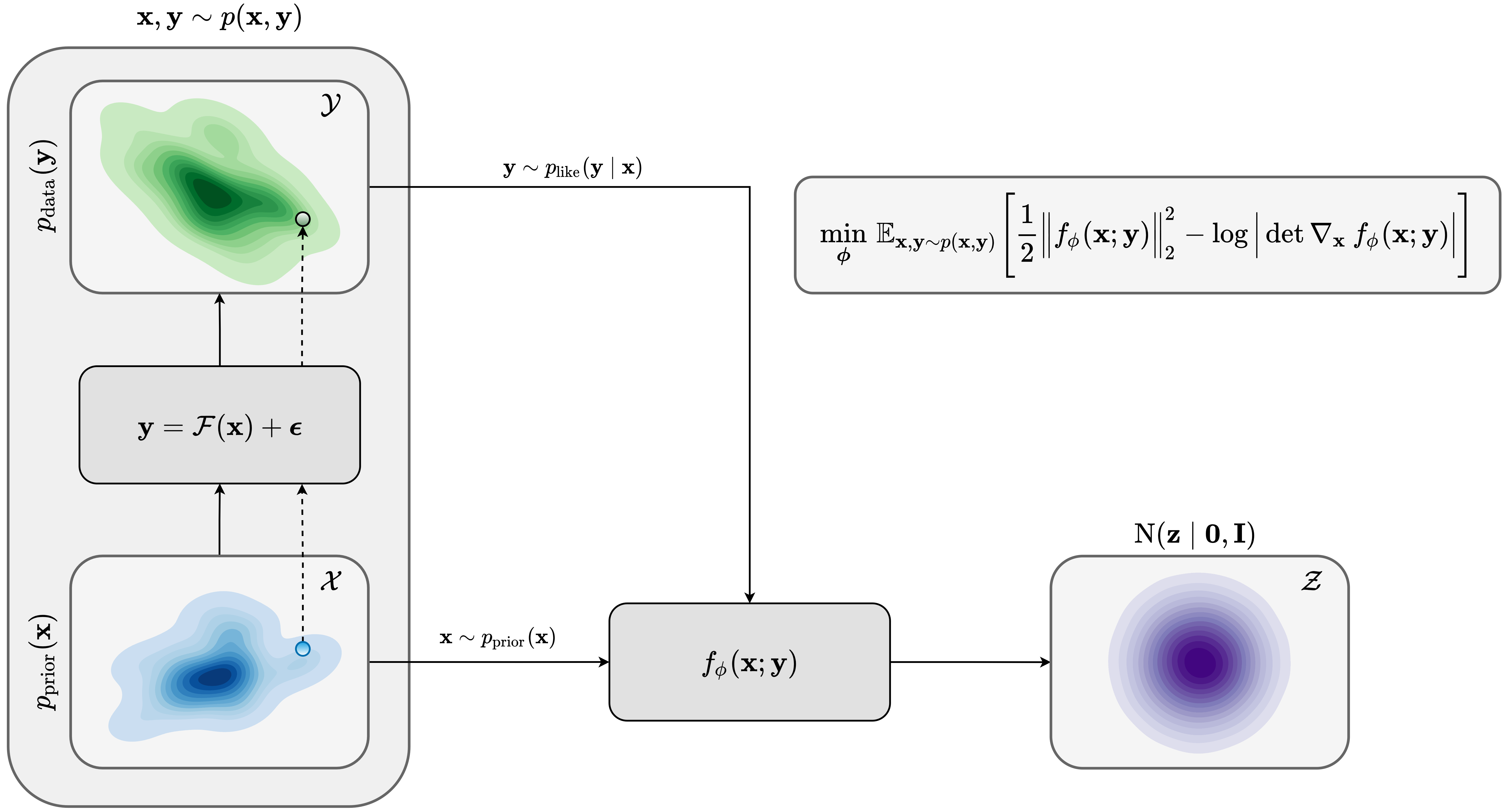
A conditional normalizing flows—in the context of amortized variational inference—aims to map input samples \(\B{z}\) from a latent standard multivariate Gaussian distribution \(\mathrm{N}(\B{z} \mid \B{0}, \B{I})\) to samples from the posterior distribution given the observed data \(\B{y} \sim p_{\text{data}}(\B{y})\) as an additional input. This nonlinear mapping can formally be stated as \(f_{\phi}^{-1}(\,\cdot\,; \B{y}): \mathcal{Z} \to \mathcal{X}\), with \(f_{\phi}^{-1}(\B{z}; \B{y})\) being the inverse of the conditional normalizing flow with respect to its first argument. Due to the low computational cost of evaluating invertible neural networks in reverse (Dinh et al., 2016), using conditional normalizing flows as a surrogate conditional distribution \(p_{\phi}(\B{x} \mid \B{y})\) allows for extremely fast sampling from \(p_{\phi}(\B{x} \mid \B{y})\). In addition to low-cost sampling, the invertibility of conditional normalizing flows permits straightforward and cheap estimation of the density \(p_{\phi}(\B{x} \mid \B{y})\). This allows for tractable amortized variational inference via equation \(\ref{vi_forward_kl}\) through the following change-of-variable formula in probability distributions (Villani, 2009), \[ \begin{equation} p_{\phi}(\B{x} \mid \B{y}) = \mathrm{N}\left(f_{\phi}(\B{x}; \B{y}) \,\bigl\vert\, \B{0}, \B{I}\right)\, \Big | \det \nabla_{\B{x}} f_{\phi}(\B{x}; \B{y}) \Big |, \quad \forall\, \B{x}, \B{y} \sim p(\B{x}, \B{y}). \label{density_estimation} \end{equation} \] In the above formula, \(\mathrm{N}\left(f_{\phi}(\B{x}; \B{y}) \,\bigl\vert\, \B{0}, \B{I}\right)\) represents the PDF for a multivariate standard Gaussian distribution evaluated at \(f_{\phi}(\B{x}; \B{y})\). Thanks to the special design of invertible neural networks (Dinh et al., 2016), density estimation via equation \(\ref{density_estimation}\) is cheap since evaluating the conditional normalizing flow and the determinant of its Jacobian \(\det \nabla_{\B{x}} f_{\phi}(\B{x}; \B{y})\) are almost free of cost. Given the expression for \(p_{\phi}(\B{x} \mid \B{y})\) in equation \(\ref{density_estimation}\), we derive the following training objective for amortized conditional normalizing flows: \[ \begin{equation} \begin{aligned} \Bs{\phi}^{\ast} & = \argmin_{\phi}\, \mathbb{E}_{(\B{x}, \B{y}) \sim p(\B{x}, \B{y})} \big[ -\log p_{\phi} (\B{x} \mid \B{y}) \big] \\ & = \argmin_{\phi}\, \mathbb{E}_{(\B{x}, \B{y}) \sim p(\B{x}, \B{y})} \Big[ \frac{1}{2} \left \| f_{\phi}(\B{x}; \B{y}) \right \|^2_2 - \log \Big | \det \nabla_{\B{x}} f_{\phi}(\B{x}; \B{y}) \Big | \Big]. \end{aligned} \label{vi_forward_kl_nf} \end{equation} \] In the above objective, the \(\ell_2\)-norm follows from a standard Gaussian distribution assumption on the latent variable, i.e., the output of the normalizing flow. The second term quantifies the relative change of density volume [papamakarios2021] and can be interpreted as an entropy regularization of \(p_{\phi}(\B{x} \mid \B{y})\), which prevents the conditional normalizing flow from converging to solutions, e.g., \(f_{\phi}(\B{x}; \B{y}) := \B{0}\). Due to the particular design of invertible networks (Dinh et al., 2016; Kruse et al., 2021), computing the gradient of \(\det \nabla_{\B{x}} f_{\phi}(\B{x}; \B{y})\) has a negligible extra cost. Figure 2 illustrates the pretraining phase as a schematic.

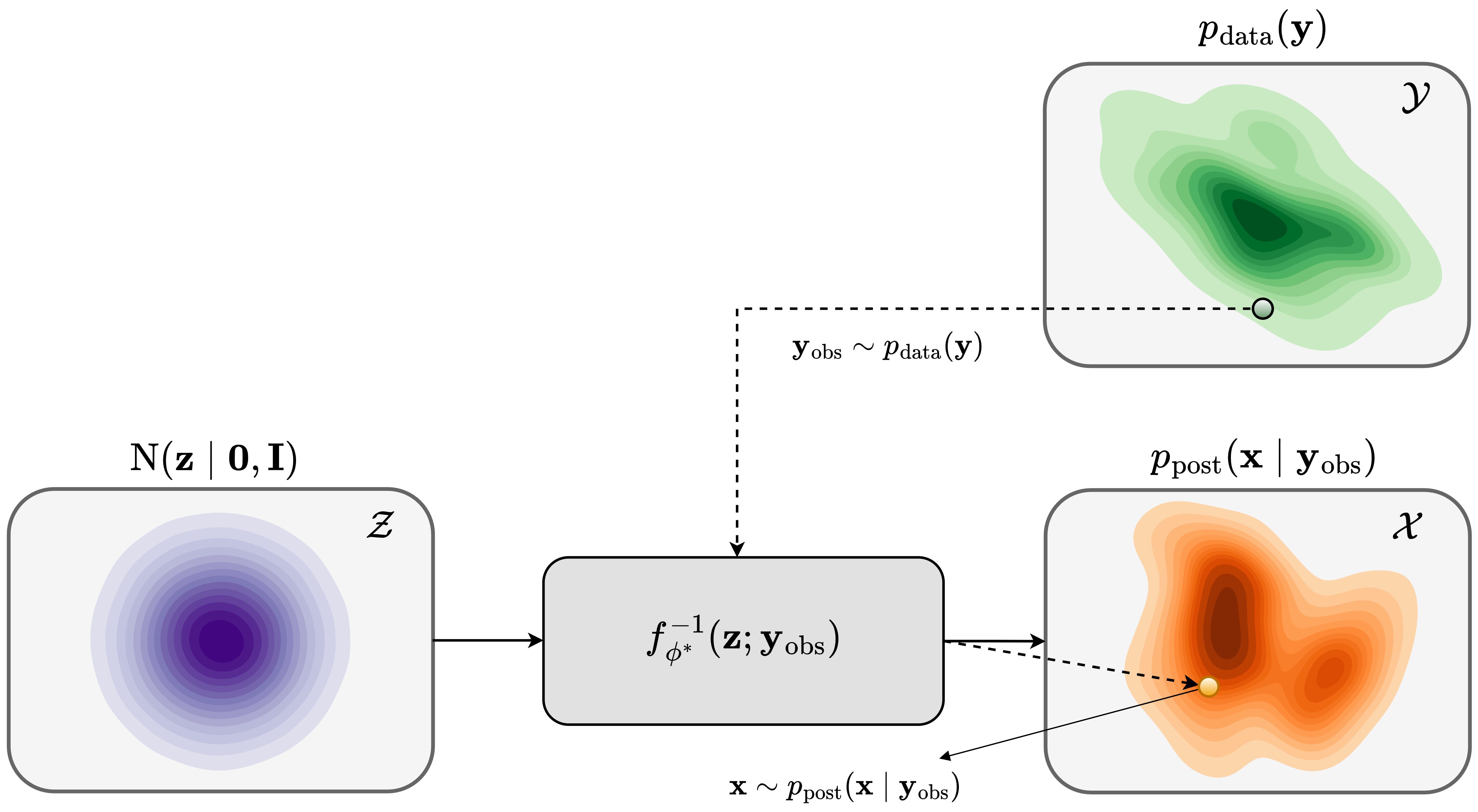
After training, given a previously unseen observed data \(\B{y}_{\text{obs}} \sim p_{\text{data}}(\B{y})\) we sample from the posterior distribution using the inverse of the conditional normalizing flow. We achieve this by feeding latent samples \(\B{z} \sim \mathrm{N} (\B{z} \mid \B{0}, \B{I})\) to the conditional normalizing flow’s inverse \(f_{\phi}^{-1}(\B{z}; \B{y}_{\text{obs}})\) while conditioning on the observed data \(\B{y}_{\text{obs}}\), \[ \begin{equation} f_{\phi}^{-1}(\B{z}; \B{y}_{\text{obs}}) \sim p_{\text{post}} (\B{x} \mid \B{y}_{\text{obs}}), \quad \B{z} \sim \mathrm{N} (\B{z} \mid \B{0}, \B{I}). \label{sampling_amortized} \end{equation} \] This step is illustrated in Figure 3. As the process above does not involve forward operator evaluations, sampling with pretrained conditional normalizing flows is fast once an upfront cost of amortized variational inference is incurred. In the next section, we apply the above amortized variational inference to a seismic imaging example in a controlled setting in which we assume no data distribution shifts during inference.

Validating amortized variational inference

The objective of this example is to apply amortized variational inference to the high-dimensional seismic imaging problem. We show that a relatively good pretrained conditional normalizing flow within the context of amortized variational inference can be used to provide approximate posterior samples for previously unseen seismic data that is drawn from the same distribution as training seismic data. We begin by introducing seismic imaging and describe challenges with Bayesian inference in this problem.

Seismic imaging

We are concerned with constructing an image of the Earth’s subsurface using indirect surface measurements that record the Earth’s response to synthetic sources being fired on the surface. The nonlinear relationship between these measurements, known as shot records, and the squared-slowness model of the Earth’s subsurface is governed by the wave equation. By linearizing this nonlinear relation, seismic imaging aims to estimates the short-wavelength component of the Earth’s subsurface squared-slowness model. In its simplest acoustic form, the linearization with respect to the slowness model—around a known, smooth background squared slowness model \(\B{m}_0\)-–leads to the following linear forward problem: \[ \begin{equation} \B{d}_i = \B{J}(\B{m}_0, \B{q}_i) \delta \B{m}^{\ast} + \boldsymbol{\epsilon}_i, \quad i = 1, \dots, N. \label{linear-fwd-op} \end{equation} \] We invert the above forward model to estimate the ground truth seismic image \(\delta \B{m}^{\ast}\) from \(N\) processed (linearized) shot records \(\left \{\B{d}_{i}\right \}_{i=1}^{N}\) where \(\B{J}(\B{m}_0, \B{q}_i)\) represents the linearized Born scattering operator (Gubernatis et al., 1977). This operator is parameterized by the source signature \(\B{q}_{i}\) and the smooth background squared-slowness model \(\B{m}_0\). Noise is denoted by \(\boldsymbol{\epsilon}_i\), and represents measurement noise and linearization errors. While amortized variational inference does not require knowing the closed from expression of the noise density to simulate pairs of data and model (e.g., it is sufficient to be able to simulate noise instances), for simplicity we assume the noise distribution is a zero-centered Gaussian distribution with known covariance \(\sigma^2 \B{I}\). Due to the presence of shadow zones and noisy finite-aperture shot data, wave-equation based linearized seismic imaging (in short seismic imaging for the purposes of this paper) corresponds to solving an inconsistent and ill-conditioned linear inverse problem (Lambaré et al., 1992; Schuster, 1993; Nemeth et al., 1999). To avoid the risk of overfitting the data and to quantify uncertainty, we cast the seismic imaging problem into a Bayesian inverse problem (Tarantola, 2005).

To address the challenge of Bayesian inference in this high-dimensional inverse problem, we adhere to our amortized variational inference framework. Within this approach, for an one-time upfront cost of training a conditional normalizing flow, we get access to posterior samples for previously unseen observed data that are drawn from the same distribution as the distribution of training seismic data. This includes data acquired in areas of the Earth with similar geologies, e.g., in neighboring surveys. In addition, in our framework no explicit prior density function needs to be chosen as the conditional normalizing flow learns the prior distribution during pretraining from the collection of seismic images in the training dataset. The implicitly learned prior distribution by the conditional normalizing flow minimizes the risk of negatively biasing the outcome of Bayesian inference by using overly simplistic priors. In the next section, we describe the setup for our amortized variational inference for seismic imaging.

Acquisition geometry

To mimic the complexity of real seismic images, we propose a “quasi”-real data example in which we generate synthetic data by applying the linearized Born scattering operator to \(4750\) 2D sections with size \(3075\, \mathrm{m} \times 5120\, \mathrm{m}\) extracted from the shallow section of the Kirchhoff migrated Parihaka-3D field dataset (Veritas, 2005; WesternGeco., 2012). We consider a \(12.5\, \mathrm{m}\) vertical and \(20\, \mathrm{m}\) horizontal grid spacing, and we augment an artificial \(125\, \mathrm{m}\) water column on top of these images. We parameterize the linearized Born scattering operator via a fictitious background squared-slowness model, derived from the Kirchhoff migrated images. To ensure good coverage, we simulate \(102\) shot records with a source spacing of \(50\, \mathrm{m}\). Each shot is recorded for two seconds with \(204\) fixed receivers sampled at \(25\, \mathrm{m}\) spread on top of the model. The source is a Ricker wavelet with a central frequency of \(30\,\mathrm{Hz}\). To mimic a more realistic imaging scenario, we add band-limited noise to the shot records, where the noise is obtained by filtering white noise with the source wavelet (Figure 5b).

Training configuration

Casting seismic imaging into amortized variational inference, as described in this paper, is hampered by the high-dimensionality of the data due to the multi-source nature of this inverse problem. To avoid computational complexities associated with directly using \(N\) shot records as input to the conditional normalizing flow, we choose to condition the conditional normalizing flow on the reverse-time migrated image, which can be estimated by applying the adjoint of the linearized Born scattering operator to the shot records, \[ \begin{equation} \delta \B{m}_{\text{RTM}} = \sum_{i=1}^{N} \B{J}(\B{m}_0, \B{q}_i)^{\top} \B{d}_i. \label{rtm} \end{equation} \] While \(\B{d}_i\) in the above expression is defined according to the linearized forward model in equation \(\ref{linear-fwd-op}\), which does not involve linearization errors, our method can handle observed data simulated from wave-equation based nonlinear forward modeling. Conditioning on the reverse-time migrated image and not on the shot records directly may result in learning an approximation to the true posterior distribution (Adler et al., 2022). While technique from statistics involving learned summary functions (S. T. Radev et al., 2022; Schmitt et al., 2021) can reduce the dimensionality of the observed data, we propose to limit the Bayesian inference bias induced by conditioning on the reverse-time migrated image via our physics-based latent variable correction approach. We leave utilizing summary functions in the context of seismic imaging Bayesian inference to future work.

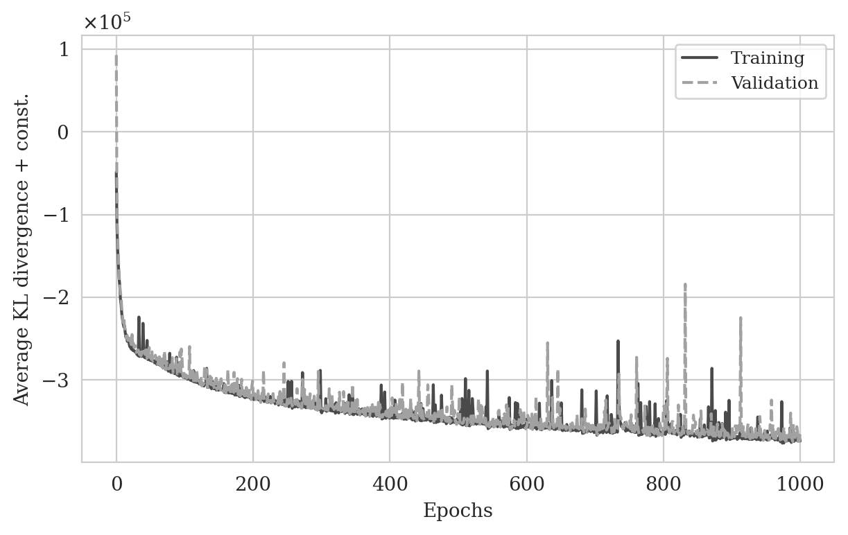
To create training pairs, \((\delta \B{m}^{(i)}, \delta \B{m}_{\text{RTM}}^{(i)}), \ i=1,\ldots,4750\), we first simulate (see Figure 2) noisy seismic data according to the above-mentioned acquisition design for all extracted seismic images \(\delta \B{m}^{(i)}\) from shallow sections of the imaged Parihaka dataset. Next, we compute \(\delta \B{m}_{\text{RTM}}^{(i)}\) by applying reverse-time-migration to the observed data for each image \(\delta \B{m}^{(i)}\). As for the conditional normalizing flow architecture, we follow Kruse et al. (2021) and use hierarchical normalizing flows due to their increased expressiveness when compared to conventional invertible architectures (Dinh et al., 2016). The expressive power of hierarchical normalizing flows is a result of applying a series of conventional invertible layers (Dinh et al., 2016) to different scales of the input in a hierarchical manner (refer to Kruse et al. (2021) for a schematic representation of the architecture). This leads to a invertible architecture with a dense Jacobian (Kruse et al., 2021) that is capable of representing complicated bijective transformations. We train this conditional normalizing flow on the pairs \((\delta \B{m}^{(i)}, \delta \B{m}_{\text{RTM}}^{(i)}), \ i=1,\ldots,4750\) according to the objective function in equation \(\ref{vi_forward_kl_nf}\) with the Adam stochastic optimization method (Diederik P Kingma and Ba, 2014) with a batchsize of \(16\) for one thousand passes over the training dataset (epochs). We use an initial stepsize of \(10^{-4}\) and decrease it after each epoch until reaching the final stepsize of \(10^{-6}\). To monitor overfitting, we evaluate the objective function at the end of every epoch over random subsets of the validation set, consisting of \(530\) seismic images extracted from the shallow sections of the imaged Parihaka dataset and the associated reverse-time migrated images. As illustrated in Figure 4, the training and validation objective values exhibit a decreasing trend, which suggests no overfitting. We stopped the training after one thousand epochs due to a slowdown in the decrease of the training and validation objective values.

Results and observations

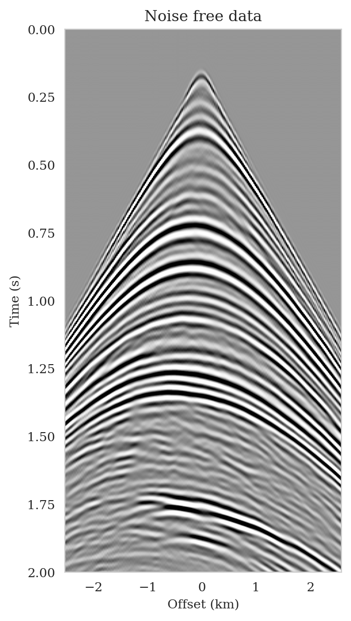
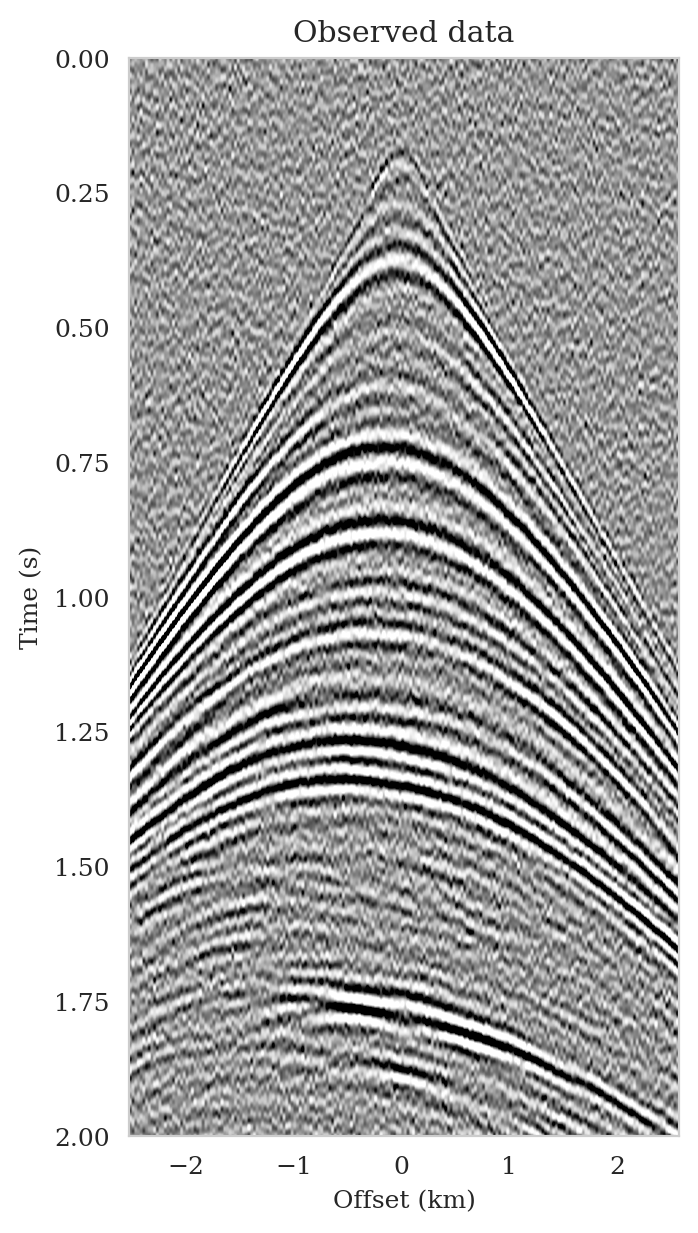
Following training, the pretrained conditional normalizing flow is able to produce samples from the posterior distribution for seismic data not used in training. These samples resemble different regularized (via the learned prior) least-squares migration images that explain the observed data. To demonstrate this, we simulate seismic data for a previously unseen perturbation model using the forward model \(\ref{linear-fwd-op}\) with the same noise variance. Figure 5 shows an example of a single noise-free (Figure 5a) and noisy (Figure 5b) shot record for one of \(102\) sources.

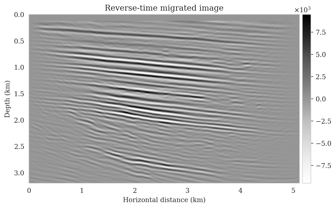
We perform reverse-time migration to obtain the necessary input for the conditional normalizing flow to obtain posterior samples. We show the ground-truth seismic image (to be estimated) and the resulting reverse-time migrated image in Figures 6a and \(\ref{rtm}\), respectively. Clearly, the reverse-time migrated image has grossly wrong amplitudes, and more importantly, due to limited-aperture shot data, the edges of the image are not well illuminated.

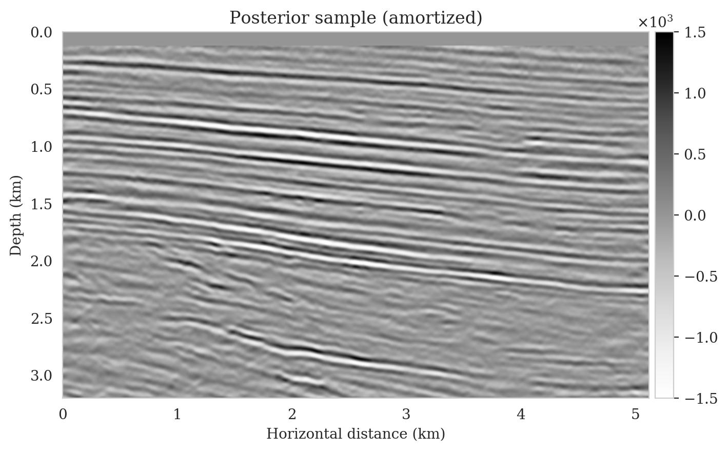
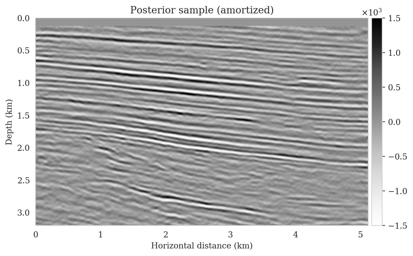
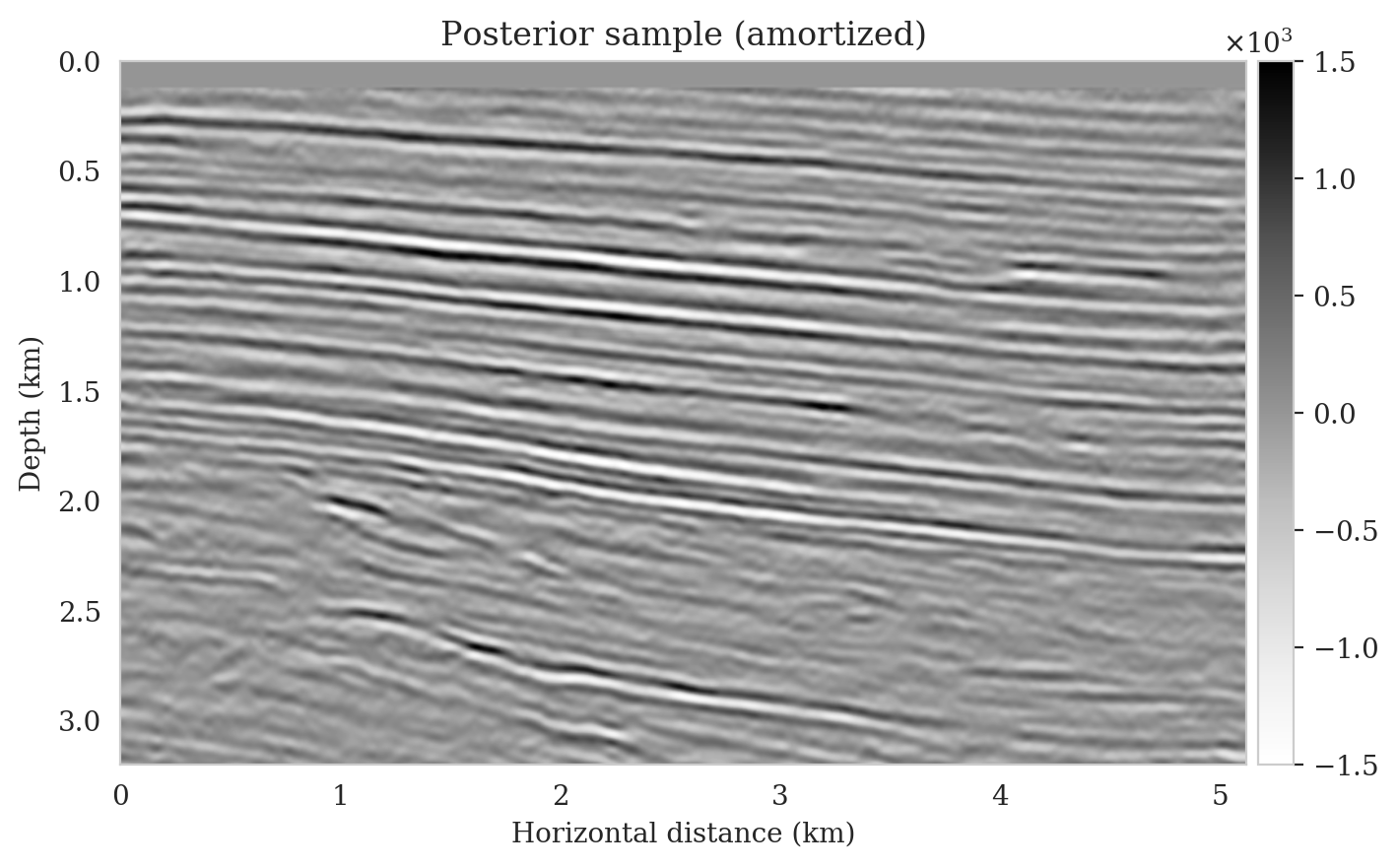
We obtain one thousand posterior samples by providing the reverse-time migrated image and latent samples drawn from the standard Gaussian distribution to the pretrained conditional normalizing flow (equation \(\ref{amortization}\)). This process is fast as it does not require any forward operator evaluations. To illustrate the variability among the posterior samples, we show six of them in Figure 7. As shown in Figure 7, these image samples have amplitudes in the same range as the ground-truth image and better predict the reflectors at the edges of the image compared to the reverse-time migration image (Figure \(\ref{rtm}\)). In addition, the posterior samples indicate improved imaging in deep regions, which is typically more difficult due to the placement of the sources and receiver near the surface.

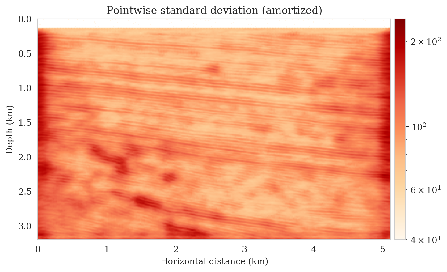
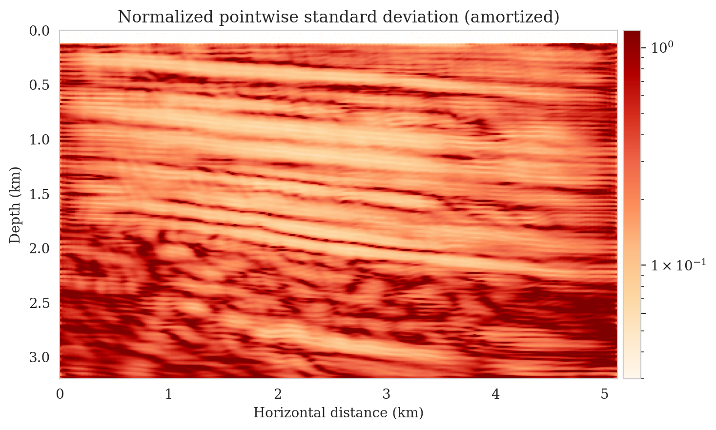
Samples from the posterior provide access to useful statistical information including approximations to moments of the distribution such as the mean and pointwise standard deviation (Figure 8). We compute the mean of the posterior samples to obtain the conditional mean estimate, i.e., the expected value of the posterior distribution. This estimate is depicted in Figure 8a. From Figure 8a, we observe that the overall amplitudes are well recovered by the conditional mean estimate, which includes partially recovered reflectors in badly illuminated areas close to the boundaries. Although the reconstructions are not perfect, they significantly improve upon the reverse-time migrations estimate. We did not observe a significant increase in the signal-to-noise ratio (SNR) of the conditional mean estimate when more than one thousand samples from the posterior are drawn. We use the one thousand samples to also estimate the pointwise standard deviation (Figure 8b), which serves as an assessment of the uncertainty. To avoid bias from strong amplitudes in the estimated image, we also plot the stabilized division of the standard deviation by the envelope of the conditional mean in Figure 8c. As expected, the pointwise standard deviation in Figures 8b and 8c indicate that we have the most uncertainty in areas of complex geology—e.g., near channels and tortuous reflectors, and in areas with a relatively poor illumination (deep and close to boundaries). The areas with large uncertainty align well with difficult-to-image parts of the model. The normalized pointwise standard deviation (Figure 8c) aims to visualize an amplitude-independent assessment of uncertainty, which indicates high uncertainty on the onset and offset of reflectors (both shallow and deeper sections), while showing low uncertainty in the areas of the image with no reflectors.

After incurring an upfront cost of training the conditional normalizing flow, the computational cost of sampling the posterior distribution is low as it does not involve any forward operator evaluations. However, the accuracy of the presented results is directly linked to the availability of high-quality training data that fully represent the joint distribution for model and data. Due to our lack of access to the subsurface of the Earth, obtaining high-quality training data is challenging when dealing with geophysical inverse problems. To address this issue, we propose to supplement amortized variational inference with a physics-based latent distribution correction technique that increases the reliability of this approach when dealing with moderate shifts in the data distribution during inference.

A physics-based treatment to data distribution shifts during inference

For accurate Bayesian inference in the context of amortized variational inference, the surrogate conditional distribution \(p_{\phi}( \B{x} \mid \B{y})\) must yield a zero amortized variational inference objective value (equation \(\ref{vi_forward_kl}\)). Achieving this objective is challenging due to lack of access to model and data pairs that sufficiently captures the underlying joint distribution in equation \(\ref{vi_forward_kl}\). Additionally, due to potential shifts to the joint distribution during inference, i.e., shifts in the prior distribution or the forward (likelihood) model (equation \(\ref{forward_model}\)), the conditional normalizing flow can no longer reliably provide samples from the posterior distribution due to lack of generalization. Under such conditions feeding latent samples drawn from a standard Gaussian distribution to the conditional normalizing flow may lead to posterior sampling errors. To quantify the posterior distribution approximation error and to propose our correction method, we will use the invariance of the KL divergence to differentiable and invertible mappings (R. Liu et al., 2014). This property relates conditional normalizing flow’s error in posterior distribution approximation to its error in Gaussianizing the input model and data pairs.

KL divergence invariance relation

The errors that the pretrained conditional normalizing flow makes in approximating the posterior distribution can be formally quantified using the invariance of the KL divergence under diffeomorphism mappings (R. Liu et al., 2014). Using this relation, we relate the posterior distribution approximation errors (KL divergence between true and predicted posterior) to the errors that the conditional normalizing flow makes in gaussianizing its inputs (KL divergence between the distribution of “gaussianized” inputs and standard Gaussian distribution). Specifically, for observed data \(\B{y}_{\text{obs}}\) drawn from a shifted data distribution \(\widehat{p}_{\text{data}} (\B{y}) \neq p_{\text{data}} (\B{y})\), the invariance relation states \[ \begin{equation} \KL\,\left(p_{\phi} (\B{z} \mid \B{y}_{\text{obs}}) \mid\mid \mathrm{N}(\B{z} \mid \B{0}, \B{I})\right) = \KL\, \left(p_{\text{post}}(\B{x} \mid \B{y}_{\text{obs}}) \mid\mid p_{\phi}(\B{x} \mid \B{y}_{\text{obs}})\right) > 0. \label{kl_divergence_invariance} \end{equation} \] In this expression, \(p_{\phi} (\B{z} \mid \B{y}_{\text{obs}})\) represents the distribution of conditional normalizing flow output \(\B{z} = f_{\phi}(\B{x}; \B{y}_{\text{obs}})\). That is, passing inputs \(\B{x} \sim p(\B{x} \mid \B{y}_{\text{obs}})\) for one instance of observed data \(\B{y}_{\text{obs}} \sim \widehat{p}_{\text{data}} (\B{y})\) to the conditional normalizing flow implicitly defines a (conditional) distribution \(p_{\phi} (\B{z} \mid \B{y}_{\text{obs}})\) in the conditional normalizing flow output space. We refer to this distribution as the shifted latent distribution as it is the result of a data distribution shift translated through the conditional normalizing flow to the latent space. The data distribution shifts can be caused by changes in number of sources, noise distribution, wavelet source frequency, and geological features to be imaged. Equation \(\ref{kl_divergence_invariance}\) states that the conditional normalizing flow fails to accurately Gaussianize the input models \(\B{x} \sim p(\B{x} \mid \B{y}_{\text{obs}})\) for the given data \(\B{y}_{\text{obs}}\). Failure to take into account the mismatch between the shifted latent distribution \(p_{\phi} (\B{z} \mid \B{y}_{\text{obs}})\) and \(\mathrm{N}(\B{z} \mid \B{0}, \B{I})\) leads to posterior sampling errors as the KL divergence between the predicted and true posterior distributions is nonzero (equation \(\ref{kl_divergence_invariance}\)). In other words, feeding latent samples drawn from a standard Gaussian distribution to \(f_{\phi}^{-1}(\B{z}; \B{y}_{\text{obs}})\) produces samples from \(p_{\phi}(\B{x} \mid \B{y}_{\text{obs}})\), which does not accurately approximate the true posterior distribution under the assumption of data distribution shift. On the other hand, with the same reasoning via the KL divergence invariance relation, feeding samples from the shifted latent distribution \(p_{\phi}(\B{z} \mid \B{y}_{\text{obs}})\) to the conditional normalizing flow yields accurate posterior samples. However, obtaining samples from \(p_{\phi}(\B{z} \mid \B{y}_{\text{obs}})\) is not trivial as we do not have a closed-form expression for its density. In the next section, we introduce a physics-based approximation to the shifted-latent distribution.

Physics-based latent distribution correction

Ideally, performing accurate posterior sampling via the pretrained conditional normalizing flow—in the presence of data distribution shifts—requires passing samples from the shifted latent distribution \(p_{\phi} (\B{z} \mid \B{y}_{\text{obs}})\) to \(f_{\phi}^{-1}(\B{z}; \B{y}_{\text{obs}})\). Unfortunately, accurately sampling \(p_{\phi} (\B{z} \mid \B{y}_{\text{obs}})\) requires access to the true posterior distribution, which we are ultimately after and do not have access to. Alternatively, we propose to quantify \(p_{\phi} (\B{z} \mid \B{y}_{\text{obs}})\) using Bayes’ rule, \[ \begin{equation} p_{\phi} (\B{z} \mid \B{y}_{\text{obs}}) = \frac{p_{\text{like}} (\B{y}_{\text{obs}} \mid \B{z})\, p_{\text{prior}} (\B{z})}{\widehat{p}_{\text{data}} (\B{y}_{\text{obs}})}, \label{bayes_rule_physic_inf} \end{equation} \] where the physics-informed likelihood function \(p_{\text{like}} (\B{y}_{\text{obs}} \mid \B{z})\) and the prior distribution \(p_{\text{prior}} (\B{z})\) over the latent variable are defined as \[ \begin{equation} \begin{aligned} - \log p_{\phi}(\B{z} \mid \B{y}_{\text{obs}}) & = - \sum_{i=1}^{N} \log p_{\text{like}} (\B{y}_{\text{obs}, i} \mid \B{z} ) - \log p_{\text{prior}} (\B{z}) + \log \widehat{p}_{\text{data}} (\B{y}_{\text{obs}}) \\ & := \frac{1}{2 \sigma^2} \sum_{i=1}^{N} \big \|\B{y}_{\text{obs}, i} - \mathcal{F}_i \circ f_{\phi}^{-1}(\B{z}; \B{y}_{\text{obs}}) \big\|_2^2 + \frac{1}{2 } \big \| \B{z} \big \|_2^2 + \text{const}. \end{aligned} \label{physics_informed_density} \end{equation} \] In the above expression, the physics-informed likelihood function \(p_{\text{like}} (\B{y}_{\text{obs}} \mid \B{z})\) follows from the forward model in equation \(\ref{forward_model}\) with a Gaussian assumption on the noise with mean zero and covariance matrix \(\sigma^2 \B{I}\), and the prior distribution \(p_{\text{prior}} (\B{z})\) is chosen as a standard Gaussian distribution with mean zero and covariance matrix \(\B{I}\). The choice of the likelihood function ensures physics and data fidelity by giving more importance to latent variables that once passed through the pretrained conditional normalizing flow and the forward operator provide smaller data misfits while the prior distribution \(p_{\text{prior}} (\B{z})\) injects our prior beliefs about the latent variable, which is by design chosen to be distributed according to a standard Gaussian distribution.

Due to our choice of the likelihood function and prior distribution above, the effective prior distribution over the unknown \(\B{x}\) is in fact a conditional prior characterized by the pretrained conditional normalizing flow (Asim et al., 2020). As observed by Y. Yang and Soatto (2018) and Orozco et al. (2021), using a conditional prior may be more informative than its unconditional counterpart because it is conditioned by the observed data \(\B{y}_{\text{obs}}\). Our approach can be also viewed as an instance of online variational Bayes (Zeno et al., 2018) where data arrives sequentially and previous posterior approximates are used as priors for subsequent approximations.

In the next section, we improve the available amortized approximation to the posterior distribution by relaxing the standard Gaussian distribution assumption of the conditional normalizing flow latent distribution.

Gaussian relaxation of the latent distribution

By definition, feeding samples from \(p_{\phi}(\B{z} \mid \B{y}_{\text{obs}})\) to the pretrained amortized conditional normalizing flows provides samples from the posterior distribution (see discussion beneath equation \(\ref{kl_divergence_invariance}\)). To maintain the low computational cost of sampling with amortized variational inference, it is imperative that \(p_{\phi}(\B{z} \mid \B{y}_{\text{obs}})\) is sampled as cheaply as possible. To this end, we exploit the fact that conditional normalizing flows in the context of amortized variational inference are trained to Gaussianize the input model random variable (equation \(\ref{vi_forward_kl_nf}\)). This suggests that the shifted latent distribution \(p_{\phi}(\B{z} \mid \B{y}_{\text{obs}})\) will be close to a standard Gaussian distribution for a certain class of data distribution shifts. We exploit this property and approximate the shifted latent distribution \(p_{\phi} (\B{z} \mid \B{y}_{\text{obs}})\) via a Gaussian distribution with an unknown mean and diagonal covariance matrix, \[ \begin{equation} p_{\phi} (\B{z} \mid \B{y}_{\text{obs}}) \approx \mathrm{N} \big(\B{z} \mid \Bs{\mu}, \operatorname{diag}(\B{s})^2\big), \quad \B{z} \in \mathcal{Z}. \label{gaussian_approximation} \end{equation} \] In the above expression, the vector \(\Bs{\mu}\) corresponds to the mean and the vector \(\operatorname{diag}(\B{s})^2\) represents a diagonal covariance matrix with diagonal entries \(\B{s} \odot \B{s}\) (with the symbol \(\odot\) denoting elementwise multiplication) that need to be determined. We estimate these quantities by minimizing the reverse KL divergence between the relaxed Gaussian latent distribution \(\mathrm{N} \big(\B{z} \mid \Bs{\mu}, \operatorname{diag}(\B{s})^2\big)\) and the shifted latent distribution \(p_{\phi}(\B{z} \mid \B{y}_{\text{obs}})\). According to the variational inference objective function associated with the reverse KL divergence in equation \(\ref{vi_reverse_kl}\), this correction can be achieved by solving the following optimization problem (see derivation in Appendix A), \[ \begin{equation} \begin{aligned} \Bs{\mu}^{\ast}, \B{s}^{\ast} & = \argmin_{\Bs{\mu}, \B{s}} \KL\,\big(\mathrm{N} \big(\B{z} \mid \Bs{\mu}, \operatorname{diag}(\B{s})^2\big) \mid\mid p_{\phi} (\B{z} \mid \B{y}_{\text{obs}}) \big) \\ & = \argmin_{\Bs{\mu}, \B{s}} \mathbb{E}_{\B{z} \sim \mathrm{N} (\B{z} \mid \B{0}, \B{I})} \bigg [\frac{1}{2 \sigma^2} \sum_{i=1}^{N} \big \| \B{y}_{\text{obs}, i}-\mathcal{F}_i \circ f_ {\phi} \big(\B{s} \odot\B{z} + \Bs{\mu}; \B{y}_{\text{obs}} \big) \big\|_2^2 \\ & \qquad \qquad \qquad \qquad \quad + \frac{1}{2} \big\| \B{s} \odot \B{z} + \Bs{\mu} \big\|_2^2 - \log \Big | \det \operatorname{diag}(\B{s}) \Big | \bigg ]. \end{aligned} \label{reverse_kl_covariance_diagonal} \end{equation} \] We solve optimization problem \(\ref{reverse_kl_covariance_diagonal}\) with the Adam optimizer where we select random batches of latent variable variables \(\B{z} \sim \mathrm{N} (\B{z} \mid \B{0}, \B{I})\) and data indices. We initialize the optimization problem \(\ref{reverse_kl_covariance_diagonal}\) by \(\Bs{\mu} = \B{0}\) and \(\operatorname{diag}(\B{s})^2 = \B{I}\). This initialization acts as a warm-start and an implicit regularization (Asim et al., 2020) since \(f_{\phi}^{-1}(\B{z}; \B{y}_{\text{obs}})\) for standard Gaussian distributed latent samples \(\B{z}\) provides approximate samples from the posterior distribution—thanks to amortization over different observed data \(\B{y}\). As a result, we expect the optimization problem \(\ref{reverse_kl_covariance_diagonal}\) to be solved relatively cheaply. Additionally, the imposed standard Gaussian distribution prior on \(\B{s} \odot \B{z} + \Bs{\mu}\) regularizes inversion for the corrections since \(\KL\,\left(p_{\phi} (\B{z} \mid \B{y}_{\text{obs}}) \mid\mid \mathrm{N}(\B{z} \mid \B{0}, \B{I})\right)\) is minimized during amortized variational inference (equation \(\ref{kl_divergence_invariance}\)). To relax the (conditional) prior imposed by the pretrained conditional normalizing flow, instead of a standard Gaussian prior, a Gaussian prior with a larger variance can be imposed on the corrected latent variable. Conditional normalizing flows’ inherent invertibility allows the normalizing flow to represent any solution \(\B{x} \in \mathcal{X}\) in the solution space. This has the additional benefit of limiting the adverse affects of imperfect pretraining of \(f_{\phi}\) in domains where access to high-fidelity training data is limited, which is often the case in practice. The output of the conditional normalizing flow can be further regularized by including additional regularization terms in equation \(\ref{reverse_kl_covariance_diagonal}\) to prevent it from producing out-of-range, non-physical results. Figure 9 summarizes our proposed method latent distribution correction method.

Inference with corrected latent distribution

Once the optimization problem \(\ref{reverse_kl_covariance_diagonal}\) is solved with respect to \(\Bs{\mu}\) and \(\B{s}\), we obtain corrected posterior samples by passing samples from the corrected latent distribution \(\mathrm{N} \big(\B{z} \mid \Bs{\mu}^{\ast}, \operatorname{diag}(\B{s}^{\ast})^2\big) \approx p_{\phi} (\B{z} \mid \B{y}_{\text{obs}})\) to the conditional normalizing flow, \[ \begin{equation} \B{x} = f_{\phi}^{-1}(\B{s}^{\ast} \odot\B{z} + \Bs{\mu}^{\ast}; \B{y}_{\text{obs}}), \quad \B{z} \sim \mathrm{N} (\B{z} \mid \B{0}, \B{I}). \label{inference_after_correction} \end{equation} \] These corrected posterior samples are implicitly regularized by the reparameterization with the pretrained conditional normalizing flow and the standard Gaussian distribution prior on \(\B{z}\) (Asim et al., 2020; Orozco et al., 2021; Siahkoohi et al., 2022b). Next section applies this physics-based correction to a seismic imaging example, in which we use the pretrained conditional normalizing flow from the earlier example.

Latent distribution correction applied to seismic imaging

The purpose of our proposed latent distribution correction approach is to accelerate Bayesian inference while maintaining fidelity to a specific observed dataset and physics. While this method is generic and can be applied to a variety of inverse problems, it is particularly relevant when solving geophysical inverse problems, where the unknown quantity is high dimensional, the forward operator is computationally costly to evaluate, and there is a lack of access to high-quality training data that represents the true heterogeneity of the Earth’s subsurface. Therefore, we apply this approach to seismic imaging to utilize the advantages of generative models for solving inverse problems, including fast conditional sampling and learned prior distributions, while limiting the negative bias induced by shifts in data distributions.

The results are presented for two cases. The first case involves introducing a series of changes in the distribution of observed data, for example changing the number of sources and the noise levels. This is followed by correcting for the error in predictions made by the pretrained conditional normalizing flow using our proposed method. In the second case, in addition to the shifts in the distribution of the observed data (forward model), we also introduce a shift in the prior distribution. We accomplish this by selecting a ground-truth image from a deeper section of the Parihaka dataset that has different image characteristics than the training images, such as tortuous reflectors and more complex geological features. In both cases, we expect the outcome of the Bayesian algorithm to improve following the correction of latent distributions described above. We provide qualitative and quantitative evaluations of the Bayesian inference results.

Shift in the forward model

In the following example, we introduce shifts in the distribution of observed data—compared to the pretraining phase—by changing the forward model. The shift involves reducing the number of sources (\(N\) in equation \(\ref{forward_model}\)) by a factor of two to four, while adding band-limited noise with 1.5 to three times larger standard deviation (\(\sigma\) in equation \(\ref{bayes_rule_log}\)). We will demonstrate the potential pitfalls of relying solely on the pretrained conditional normalizing flows in circumstances where the distribution of observed data has shifted. With the use of our latent distribution correction, we will demonstrate that we are able to correct for errors that are made by the pretrained conditional normalizing flow as a result of changes to data distribution.

Following the description of the problem setup, we will also provide comparisons between the conditional mean estimation quality before and after the latent distribution correction step. Before moving on to our results relating to uncertainty quantification on the image, we demonstrate the importance of the correction step by visualizing the improvements in fitting the observed data. Lastly, we perform a series of experiments to verify our Bayesian inference results.

Problem setup

To induce shifts in the data distribution, we reduce the number of sources and increase the standard deviation of the added band-limited noise. Consequently, we have reduced the amount of data (due to having fewer source experiments) and decreased the SNR of each shot record (due to being contaminated with stronger noise). As a consequence, seismic imaging becomes more challenging, i.e., more difficult to estimate the ground truth image, and it is expected that the uncertainty associated with the problem will also increase.

We use the same ground-truth image as in the previous example (Figure 6a), while experimenting with 25, 51, 102 sources and adding band-limited noise that has \(1.5\), \(2.0\), \(2.5\), and \(3.0\) times larger standard deviation than the pretraining setup. For each combination of source number and noise level (\(12\) combinations in total), we compute the reverse-time migrated image corresponding to that combination. Next, we perform latent distribution corrections for each of the \(12\) seismic imaging instances. All latent distribution correction optimization problems (equation \(\ref{reverse_kl_covariance_diagonal}\)) are solved using the Adam optimization algorithm (Diederik P Kingma and Ba, 2014) for five passes over the shot records (epochs). We did not observe a significant decrease in the objective function after five epochs. The objective function is evaluated each iteration by drawing a single latent sample from the standard Gaussian distribution and randomly selecting (without replacement) a data index \(i \in \{1, \ldots, 25 \}\). We use a stepsize of \(10^{-1}\) and decrease it by a factor of \(0.9\) at the end of every two epochs.

After solving the optimization problem \(\ref{reverse_kl_covariance_diagonal}\) for the different seismic imaging instances, we obtain corrected posterior samples for each instance. The next section provides a detailed discussion of the latent distribution correction that was applied to one such instance that had a significant shift in data distribution.

Improved Bayesian inference via latent distribution correction

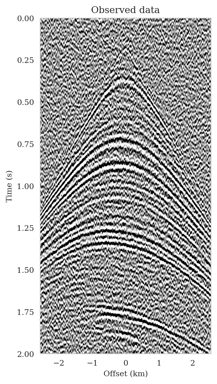
The aim of this section is to demonstrate how latent distribution correction can be used to mitigate errors induced by data distribution shifts. Specifically, we present the results for the case where the number of sources is reduced by a factor of four (\(N = 25\)) as compared to the pretrained data generation setup. The \(25\) sources are spread periodically over the survey area with a source sampling of approximately \(200\) meters. Moreover, we contaminate the resulting shot records with band-limited noise with an increased standard deviation of \(2.5\) times when compared to the pretraining phase. The overall SNR for the data thus becomes \(-2.78\,\mathrm{dB}\), which is \(7.95\,\mathrm{dB}\) lower that the SNR of the observed data during pretraining (Figure 5b). Figure 10 shows one of the `25 shot records.

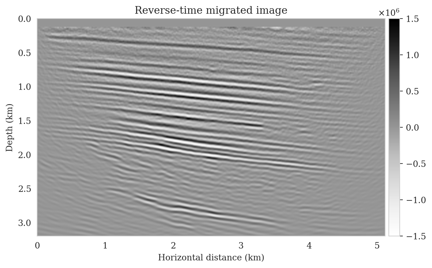
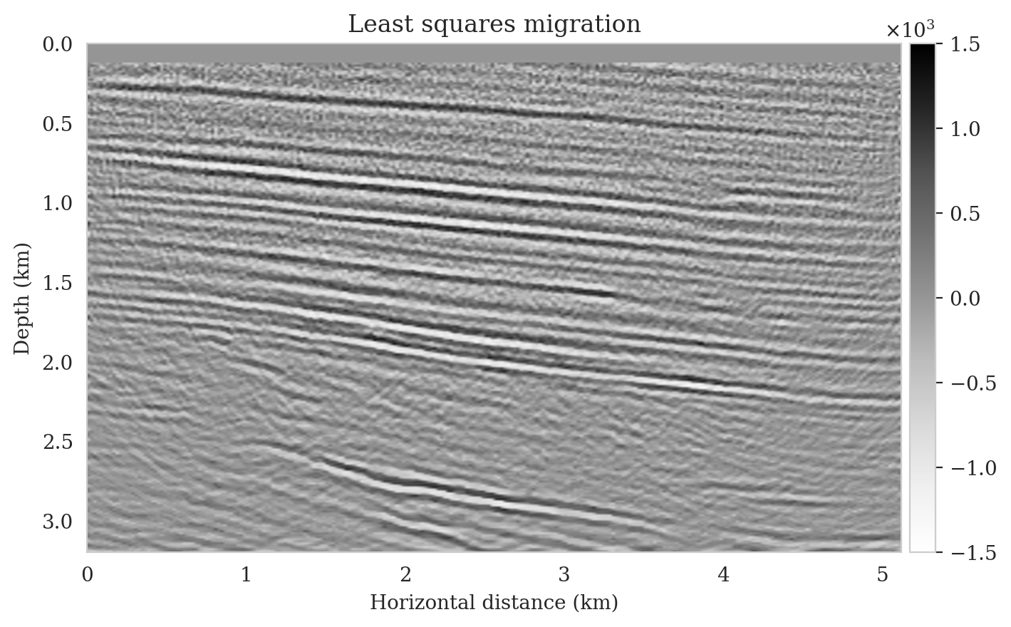
Utilizing the above observed dataset, we compute the reverse-time migrated image as an input to our pretrained conditional normalizing flow (Figure 11a). In contrast to the reverse-time migrated image shown in Figure 5b, this migrated image is, as expected, noisier, and it displays visible near-source imaging artifacts as a result of coarse source sampling. Additionally, we compute the least-squares migrated seismic image that is obtained by minimizing the negative-log likelihood (see the likelihood term in equation \(\ref{bayes_rule_log}\)). This image, shown in Figure 11b, was constructed by fitting the data without incorporating any prior information. It is evident from this image that there are strong artifacts caused by noise in the data, underscoring the importance of incorporating prior knowledge into solving seismic imaging.

Improvements in posterior samples and conditional mean estimate

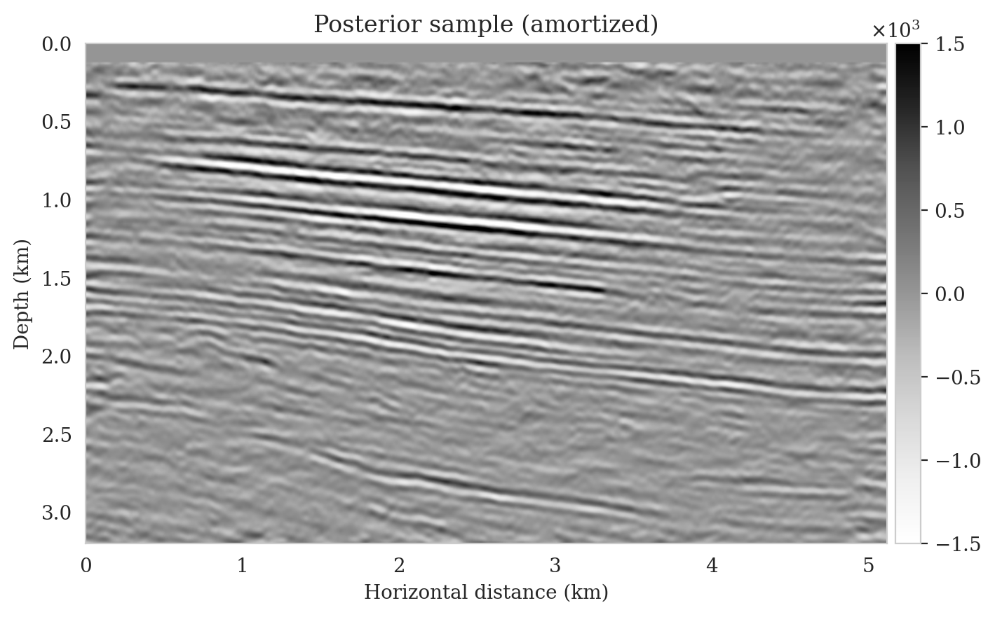
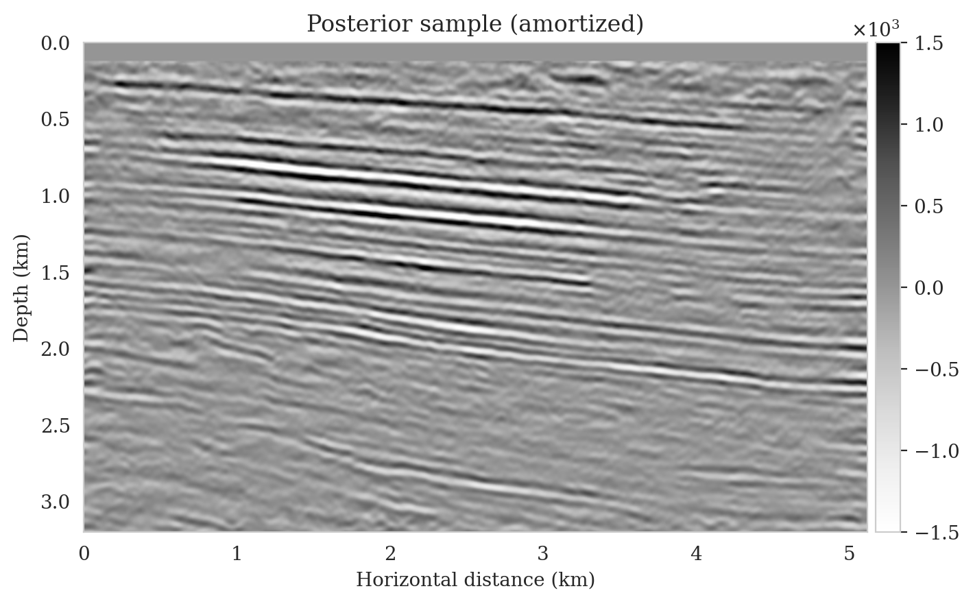
To obtain amortized (uncorrected) posterior samples, we feed the reverse-time migrated image (Figure 11a) and latent samples drawn from the standard Gaussian distribution to the pretrained normalizing flow. These samples, which are shown in the left column of Figure 12, contain artifacts near the top of the image. These artifacts are related to the near-source reverse-time migrated image artifacts (Figure 11a). Since the reverse-time migrated images used during pretraining do not contain near-source imaging artifacts—due to fine source sampling—the pretrained normalizing flow fails to eliminate them. Further, the uncorrected posterior samples do not accurately predict reflectors as they approach the boundaries and deeper sections of the image.

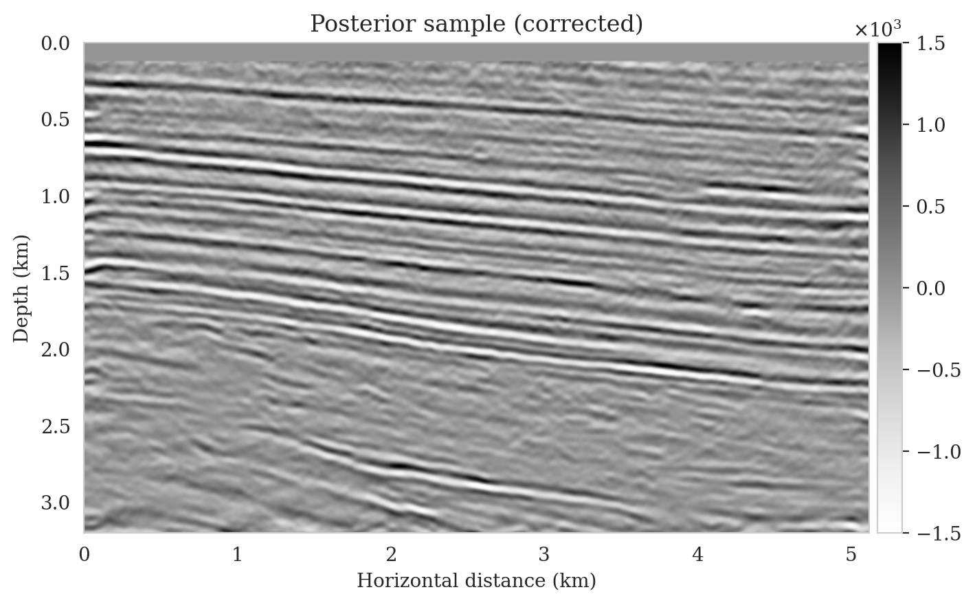
To illustrate the improved posterior sample quality following latent distribution correction, we feed latent samples drawn from the corrected latent distribution to the pretrained normalizing flow (right column of Figure 12). Comparing the left and right columns in Figure 12 indicates an improvement in the quality of samples from the posterior distribution, which can be attributed to the attenuation of near-top artifacts and an improvement in the image quality close to the boundary and deeper reflectors in the image. Moreover, the SNR values of the posterior samples after correction are approximately \(3\,\mathrm{dB}\) higher, which represents a significant improvement.

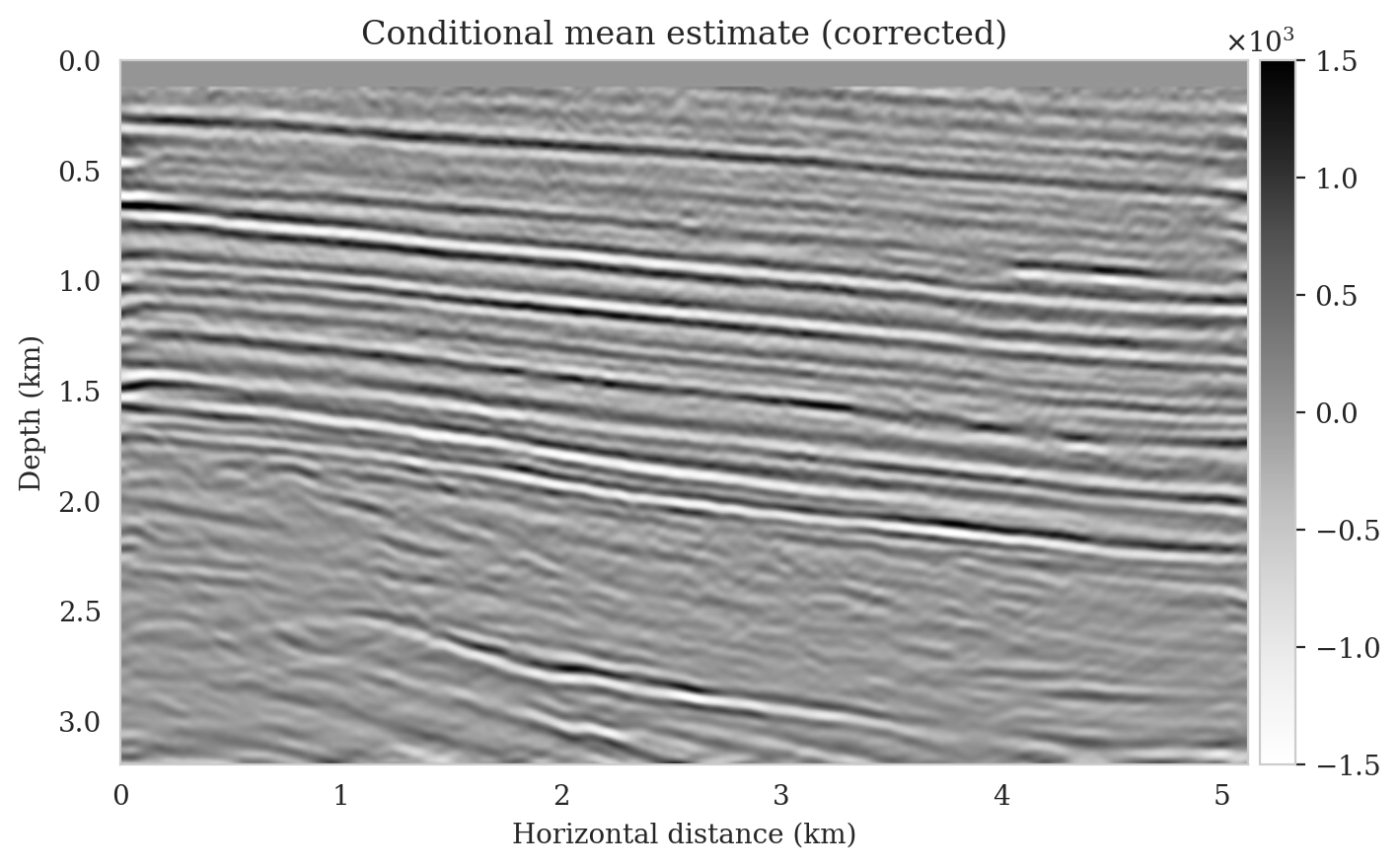
To compute the conditional mean estimate, we simulate one thousand posterior samples before and after latent distribution correction. As with the posterior samples before correction, drawing samples after correction is very cheap once the correction is done as it only requires evaluating the conditional normalizing flow over the corrected latent samples. Figures 13a and 13b show conditional mean estimates before and after latent distribution correction, respectively. The conditional mean estimate before correction reveals similar artifacts as the posterior samples before correction, in particular, near-top imaging artifacts due to coarse sources sampling and less illumination of reflectors located closer to the boundary and deeper portions of the image. The importance of our proposed latent distribution correction can be observed by juxtaposing the conditional mean estimate before (Figure 13a) and after correction (Figure 13b). The conditional mean estimate obtained after latent distribution correction eliminates the aforementioned inaccuracies and enhances the quality of the image by approximately \(4\,\mathrm{dB}\). We gain similar improvements in SNR compared to the least-squares migrated image (Figure 11b) with virtually the same cost, i.e., five passes over the shot records. This is significant improvement in SNR also is complimented by access to information regarding the uncertainty of the image.

Data-space quality control

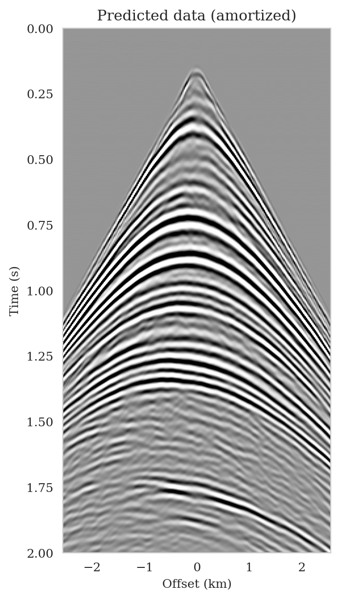
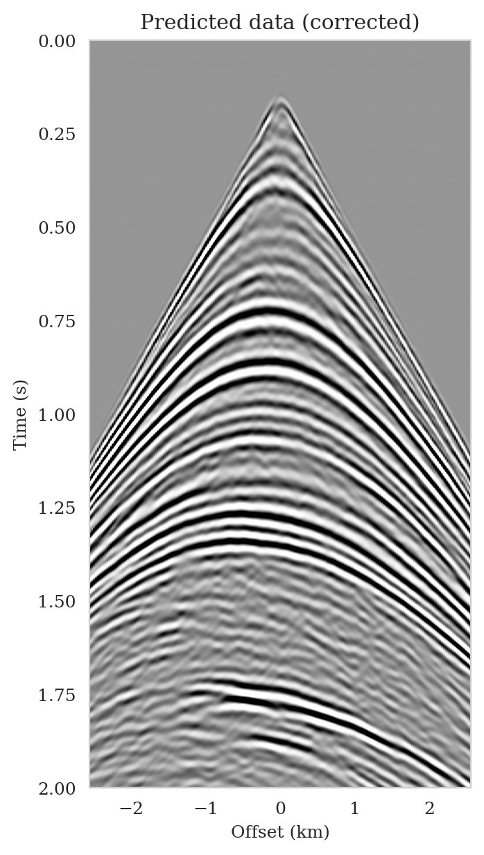
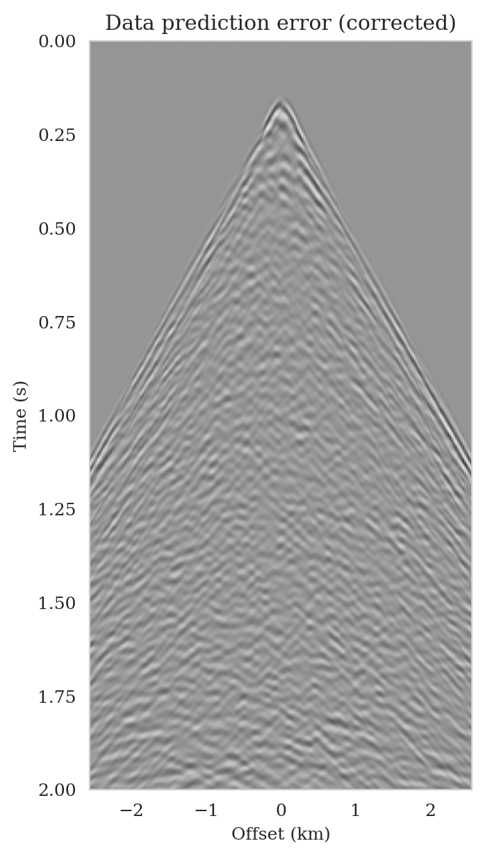
As the latent distribution correction step involves finding latent samples that are better suited to fit the data (equation \(\ref{reverse_kl_covariance_diagonal}\)), we can expect an improvement in fitting the observed data after correction. Predicted data is obtained by applying the forward operator to the conditional mean estimates, before and after latent distribution correction. Figures 14a and 14b show the predicted shot records before and after correction, respectively. In spite of the fact that both predicted data appear to be similar to ideal noise-free data (Figure 10a), the data residual associated with the conditional mean without correction reveals several coherent events that contain valuable information about the unknown seismic image. The latent distribution correction allows us to fit these coherent events as indicated by the data residual associated with the corrected conditional mean estimate.

Uncertainty quantification—pointwise standard deviation and histograms

We exploit cheap access to corrected samples from the posterior in order to extract information regarding uncertainty in the image estimates. Figure 15a displays the pointwise standard deviation among the one thousand corrected posterior samples. The overprint by the strong reflectors can be reduced by normalizing the standard deviation using a stabilized division by the conditional mean (Figure 15b). The pointwise standard deviation plots indicate high uncertainty in areas near the boundaries of the image and in the deep parts of the image where illumination is relatively poor. This observation is more evident in Figure 16, which displays three vertical profiles as \(99\%\) confidence intervals (orange colored shading) illustrating the expected increasing trend of uncertainty with depth. We additionally observe that the ground truth (dashed black) falls within the confidence intervals for most of the areas.

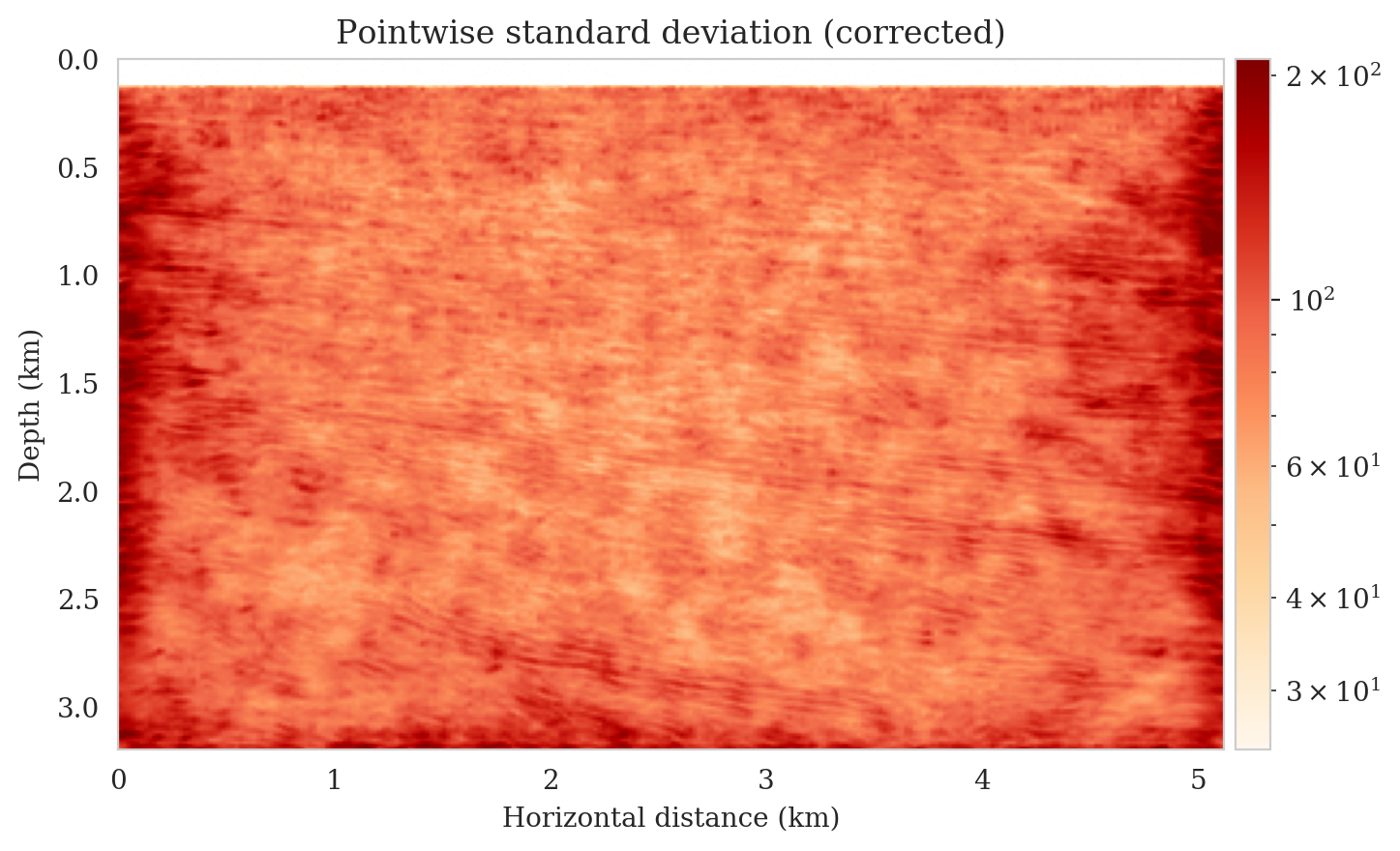
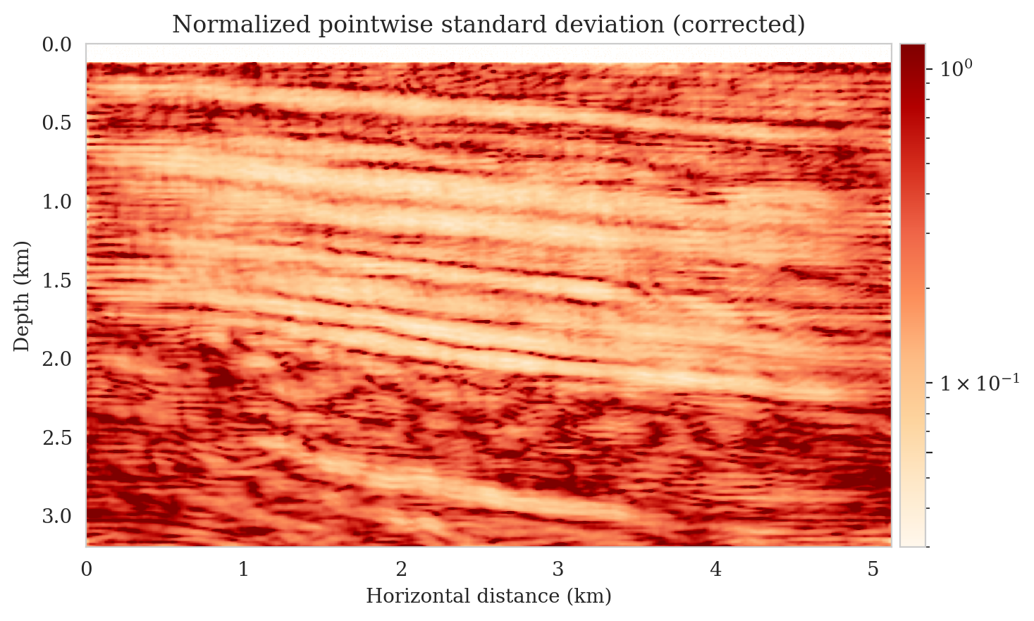
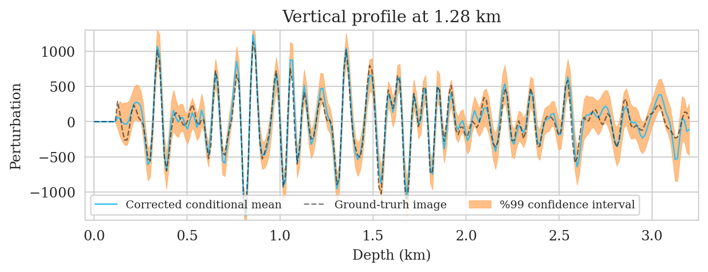
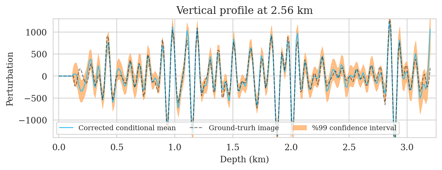
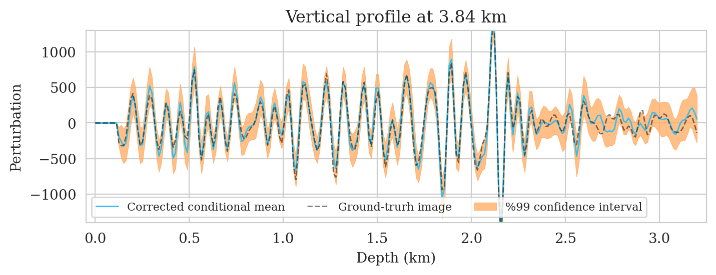
To demonstrate how the corrected posterior is informed by the observed data, we calculated histograms at three locations in Figure 15a. Prior histograms are calculated by feeding latent samples drawn from the standard Gaussian distribution to the pretrained conditional normalizing flow without using data conditioning (see Kruse et al. (2021) and Siahkoohi and Herrmann (2021) for more information). These samples in the image spaces are indicative of samples from the prior distribution implicitly learned by the conditional normalizing flow during pretraining. The resulting prior histograms are shown in Figure 17. Corresponding histograms are also obtained for the uncorrected amortized posterior distribution (equation \(\ref{sampling_amortized}\)). As mentioned before, the uncorrected posterior distribution serves as an implicit conditional prior for the subsequent step of correction of the latent distribution. The green histograms in Figure 17 represent the uncorrected amortized posterior distribution. A similar procedure is followed to obtain histograms after latent distribution correction (blue histograms). As expected, the histograms of the posterior distribution are considerably narrower than those of the learned prior, which indicates that the posterior is further informed by the specific observed dataset and physics. As a means of evaluating the effect of latent distribution correction, we provide a vertical solid line showing the ground truth value’s location. All three corrected posterior histograms for each location are shifted towards the ground truth, and their (conditional) mean plotted with the dashed vertical line indicates improved recovery of the ground truth. Compared to the amortized uncorrected histograms, the corrected histograms in Figures 17a – 17b are further contracted, suggesting that the latent distribution correction step has further informed the inference by the data.

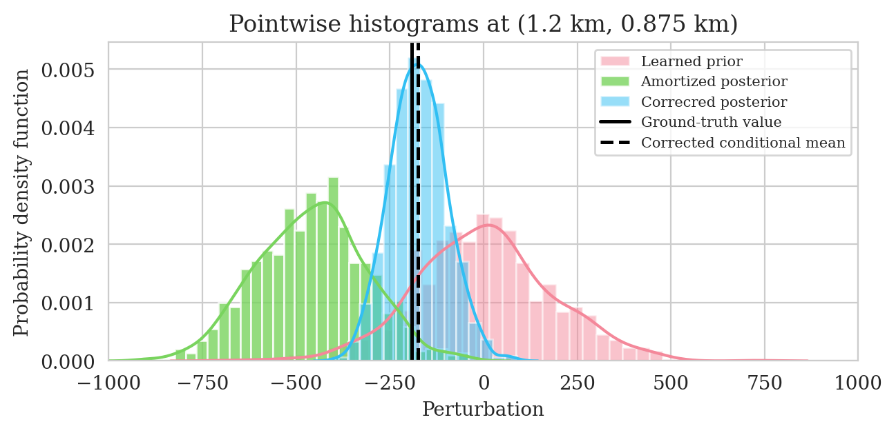
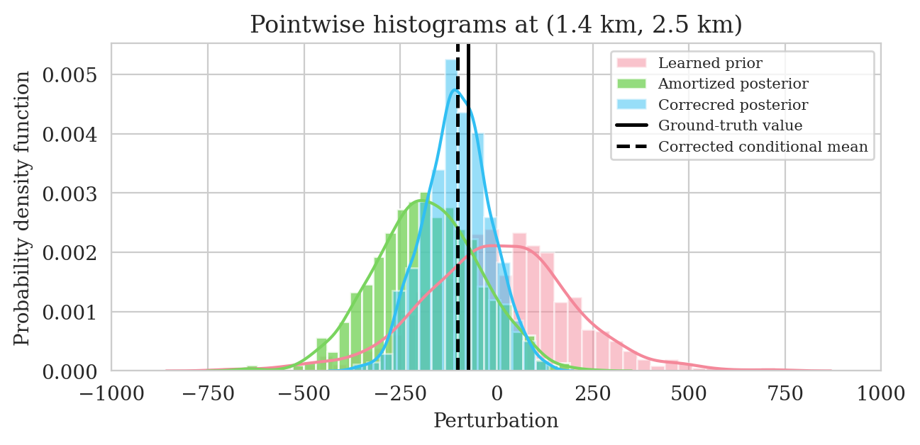
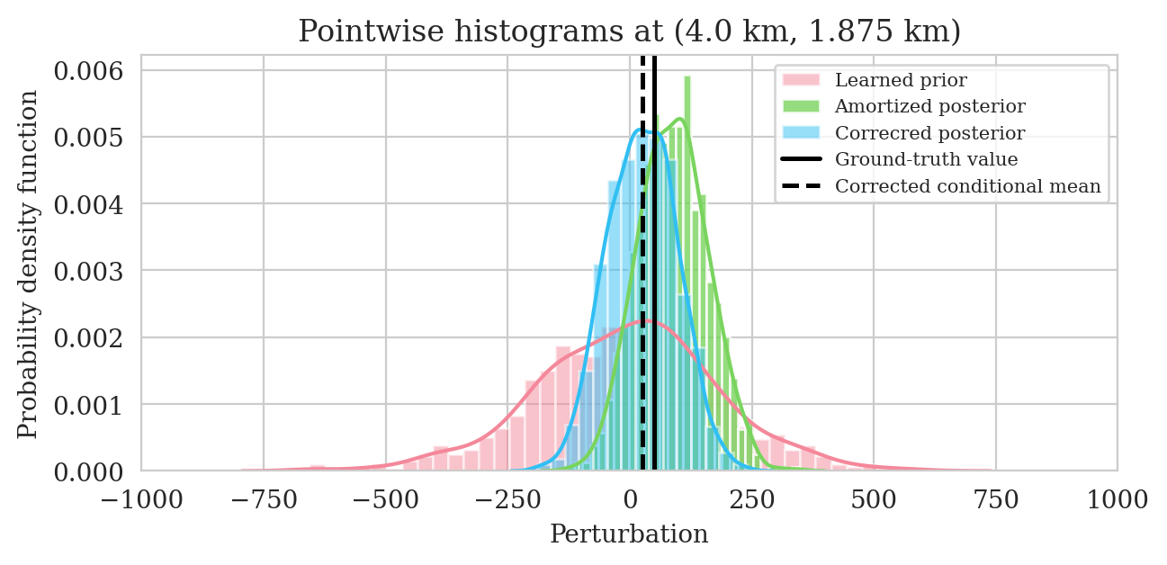
Bayesian inference verification

While we investigated the accuracy of the conditional mean estimate after correction, we do not have access to the underlying true posterior distribution to verify our proposed posterior sampling method. This is partly due to our learned prior and the implicit conditional prior used in latent variable correction, which make traditional MCMC-based comparisons challenging. To further validate our Bayesian inference procedure, we conduct a series of experiments in which we investigate the effect of gradual increase in the number of sources (\(N\)) and reduction of the noise level. As the number of sources increases and the noise level decreases, we expect to see an increase in seismic image quality and a decrease in uncertainty.

Estimation accuracy

The accuracy of the Bayesian parameter estimation method is directly affected by the amount of data that has been collected (Tarantola, 2005). That is to say with more observed data (larger \(N\)), we should be able to obtain a more accurate seismic image estimate. The same principle allows us to stack out noise when increasing the fold in seismic data acquisition. In order to assess whether our Bayesian inference approach has this property, we repeat the latent distribution correction process while varying the number of sources (using \(N = 25, 51, 102\) sources) and the amount of band-limited noise (standard deviations \(1.5, 2.0, 2.5\), and \(3.0\) times greater than the noise standard deviation during pretraining). Each of the \(12\) instances of latent distribution correction problems is treated similarly with respect to the number of passes made over the shot records and other optimization parameters. For each of the \(12\) combinations of source numbers and noise levels, we calculate the corrected conditional mean estimate and plot the SNRs as a function of the noise’s standard deviation in Figure 18.

For a fixed number of sources (\(25\), \(51\), and \(102\) sources shown with red, green, and blue colors respectively), we plot the corrected conditional means SNR as a function of the noise standard deviation. There is a clear increase in SNR trend as we decrease the noise level. In the same way, for each fixed noise level, the SNR increases with the number of sources. This verifies the our Bayesian inference method yields a more accurate estimate of the conditional mean for larger number of sources and smaller noise levels.

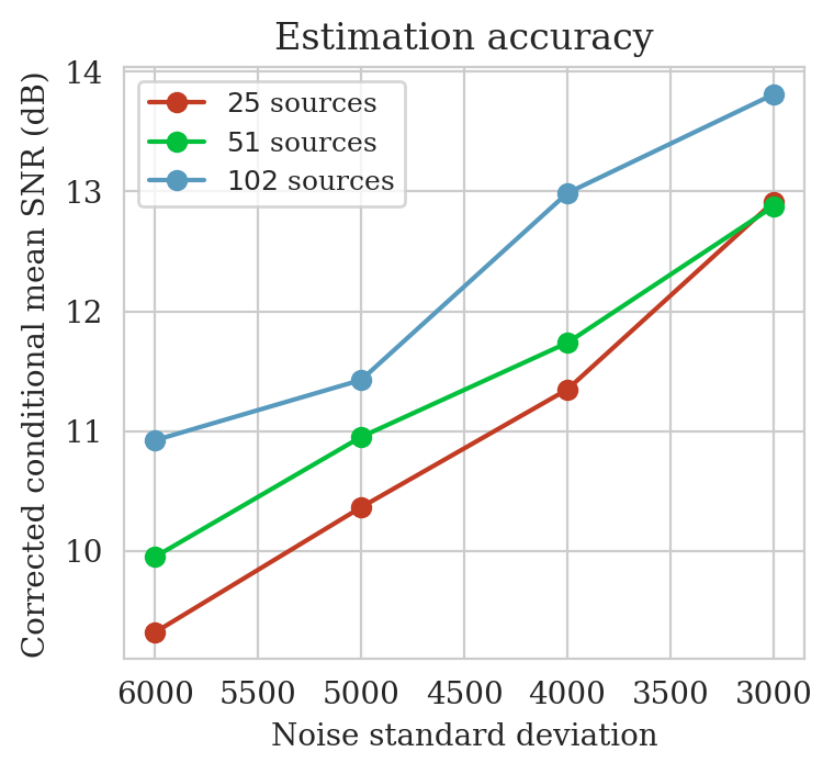
Bayesian posterior contraction

An alternative Bayesian inference verification method involves analyzing the Bayesian posterior contraction, that is, the decrease of uncertainty with more data. To examine whether or not our Bayesian inference method possesses this property, we visually inspect the resulting pointwise standard deviation plots in Figure 19 for the \(12\) possible combinations of source numbers and noise levels. Each row corresponds to the pointwise standard deviation plot for a fixed noise standard deviation (\(\sigma\)), where the number of sources (\(N\)) decreases from left to right. In each column, we maintain the number of sources and we plot the pointwise standard deviation as we increase the noise standard deviation from top to bottom. There is a consistent increase in standard deviation values as we move from the top-left to the bottom-right corner. In other words, the posterior contract (shrinks) when we have more data (more numbers of sources, Figure 19 from right to left) and when we have less noise (Figure 19 from bottom to top), which effectively means more data.

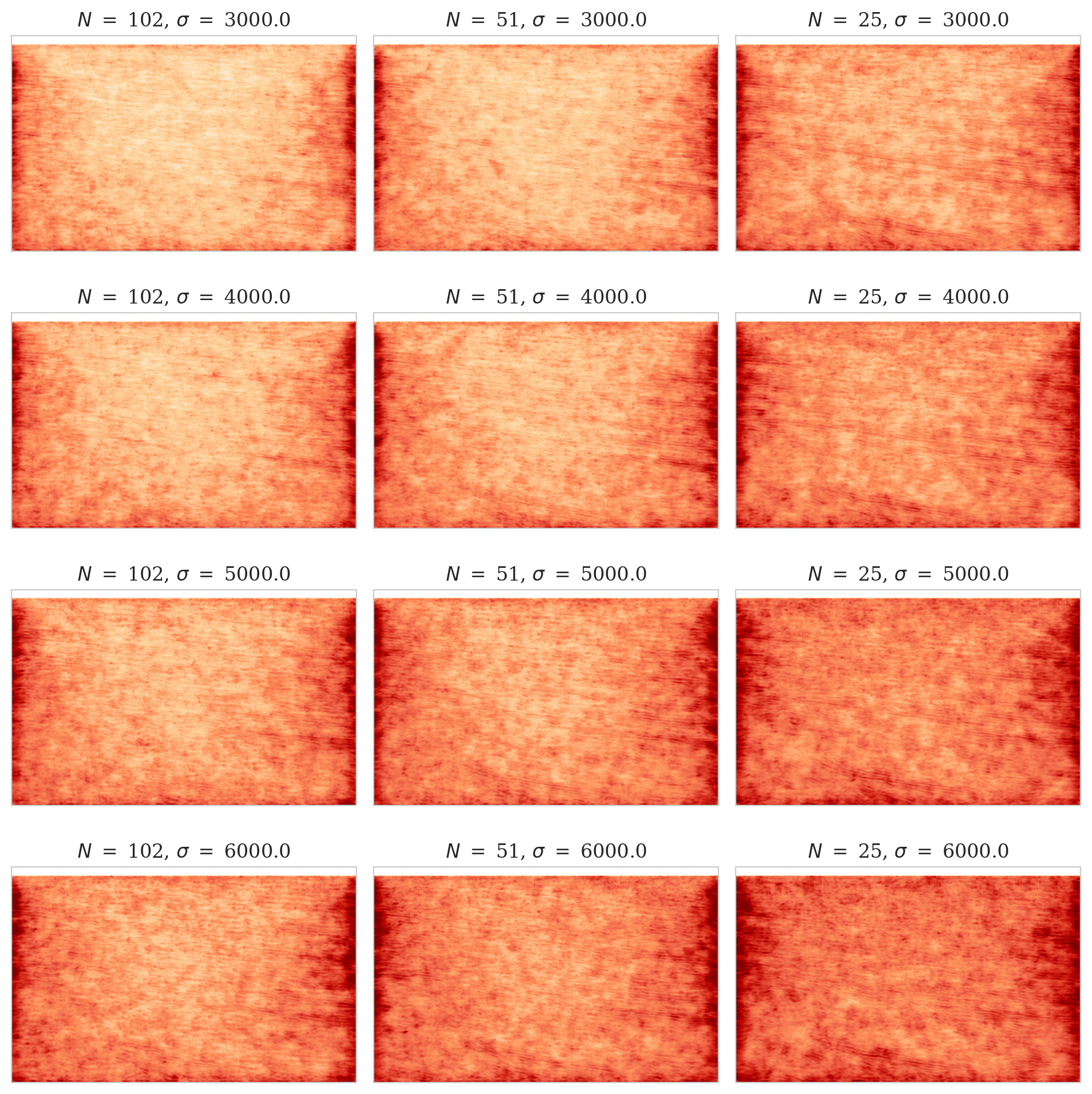
Figure 20 offers an alternate method of visualizing posterior contraction, displaying box plots of the standard deviation values for each of the \(12\) images in Figure 19. In each of the three box plots, the vertical axis corresponds to the noise standard deviation, and the horizontal axis represents the possible values in the posterior pointwise standard deviation plots. The box indicates the values that are between the first and third quartiles (where half of the possible values fall) and the line in the middle indicates the median value. Figures 20a to 20c show box plots for experiments with \(25\), \(51\), and \(102\) sources, respectively, with each box plot color reflecting a particular noise level. In each of the Figures 20a to 20c, we observe a decrease in the range of posterior standard deviation values, including median and quantiles, as we lower the noise level from left to right. Similarly, for the same noise levels, that is, box plots of the same color, the standard deviations decrease from Figure 20a to Figure 20c (increasing number of sources). The observed trends in Figures 19 and 20 verify that our Bayesian inference method exhibits the Bayesian posterior contraction property.

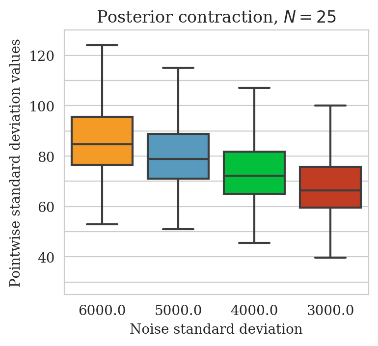
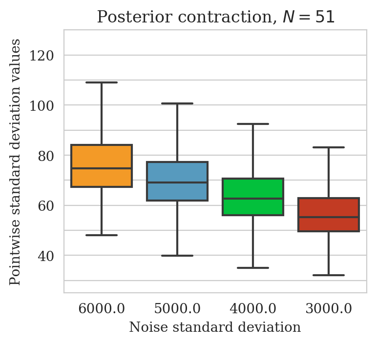
Shift in the forward model and prior distribution

This example is intended to demonstrate how our latent distribution correction method can perform Bayesian inference when the unknown ground truth image has properties that differ from the seismic images in the pretraining dataset. This expectation is based on the invertible nature of conditional normalizing flows, which allows them to represent any image in the image space (Asim et al., 2020).

As a means to mimic this scenario, unlike images used in pretraining, we have extracted two 2D seismic images from deeper sections of the Parihaka dataset. In these sections, there are fewer continuous reflectors and more complex geological features. Figures 21a and 21b show two images with drastically different geological features when compared to Figure 6a. Following the pretraining data acquisition setup, we add a water column on top of these images to reduce the near-source artifacts. Similar to the previous experiment involving forward model shifts, we use only 25 sources with 200 meters sampling distance and add noise with a \(2.5\) fold larger standard deviation than during the pretraining phase. With this setup, the noisy observed data associated with experiments involving seismic images in Figures 21a and 21b have a SNR of \(-1.56\,\mathrm{dB}\) and \(-2.41\,\mathrm{dB}\), respectively.

As part of our analysis, we compute the reverse-time (second row in Figure 21) and least-squares (third row in Figure 21) migrated images for these two ground-truth images, where the former images serve as inputs to the pretrained conditional normalizing flows. Similar to the previous example, the reverse-time migrated images contain the near-source artifacts and are contaminated by the input noise. Moreover, the least-squares migrated images highlight the importance of including prior information in this imaging problem, since this image contains strong noise-related artifacts, which might impact downstream tasks, such as horizon tracking.

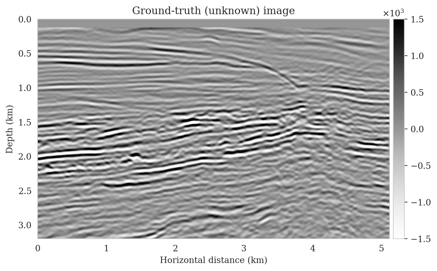
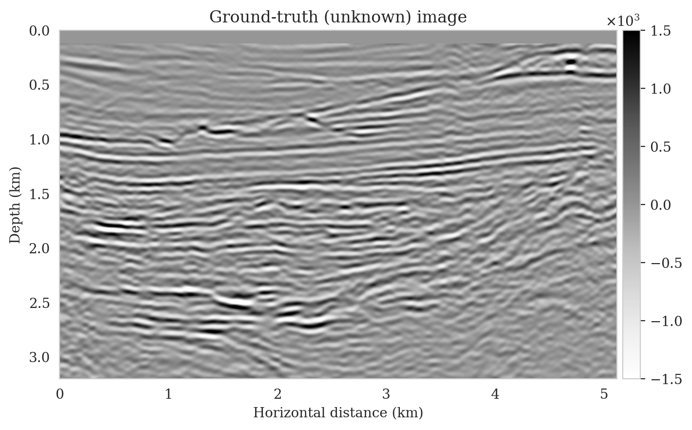
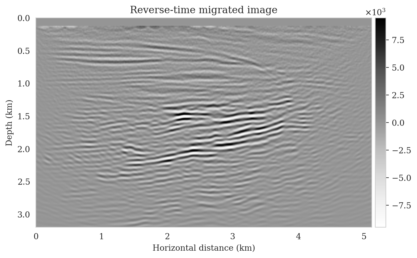
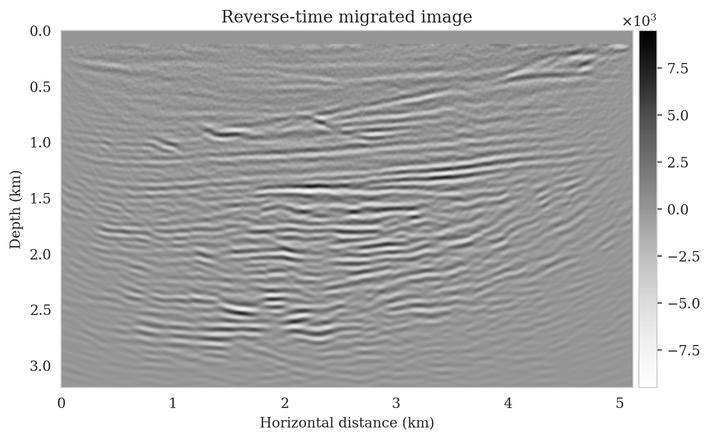
Conditional mean and pointwise standard deviations

To obtain samples from the posterior distribution, we feed the reverse-time migrated images (Figures 21c and 21d) into the pretrained conditional normalizing flow. The posterior is sampled using either standard Gaussian distributions or corrected latent samples. It is apparent, once more, that the uncorrected conditional mean estimates are significantly contaminated by artifacts in the near-source region (Figures 22a and 22b). Another type of noticeable error in these predicted images includes lower amplitudes in deeper and closer to boundary reflectors. A comparison of the conditional means estimates before (Figures 22a and 22b) and after (Figures 22c and 22d) latent distribution correction indicates attenuation of near-source artifacts as well as an improvement in reflector illumination near the boundary and deeper sections where images are more difficult to capture. Following latent distribution correction, the conditional mean estimate SNR is improved by three to four decibels for both images. To provide more quantitative results, we ran the experiments as set up in this section for eight additional seismic images sampled from deeper sections of the Parihaka dataset, sampled from deeper sections of the Parihaka dataset. The SNR of the estimated seismic images before and after latent distribution are \(5.91 \pm 0.49\,\mathrm{dB}\) and \(9.15 \pm 0.73\,\mathrm{dB}\), respectively.

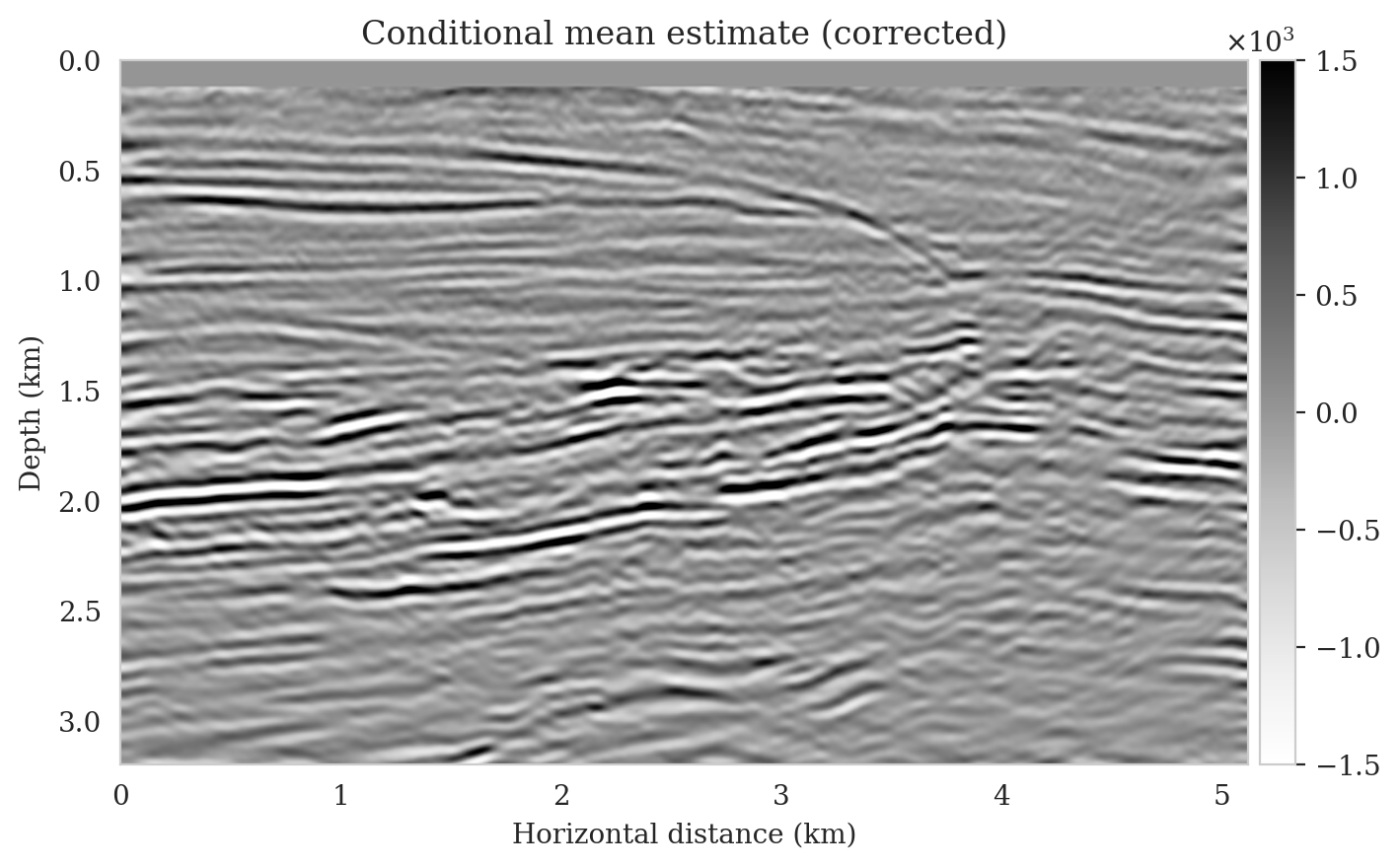
Careful inspection at the boundaries in the corrected conditional mean estimates reveals some nonrealistic events near the boundaries. The plots of pointwise standard deviations (Figures 23a and 23b) associated with corrected conditional means, however, clearly indicate that there is uncertainty for these events. This illustrates the importance of uncertainty quantification and not relying on a single estimate when addressing ill-posed inverse problems. To diminish the imprint of strong reflectors in the pointwise standard deviations plots, we also display these images when normalized with respect to the envelopes of the conditional mean estimates in Figures 23c and 23d.

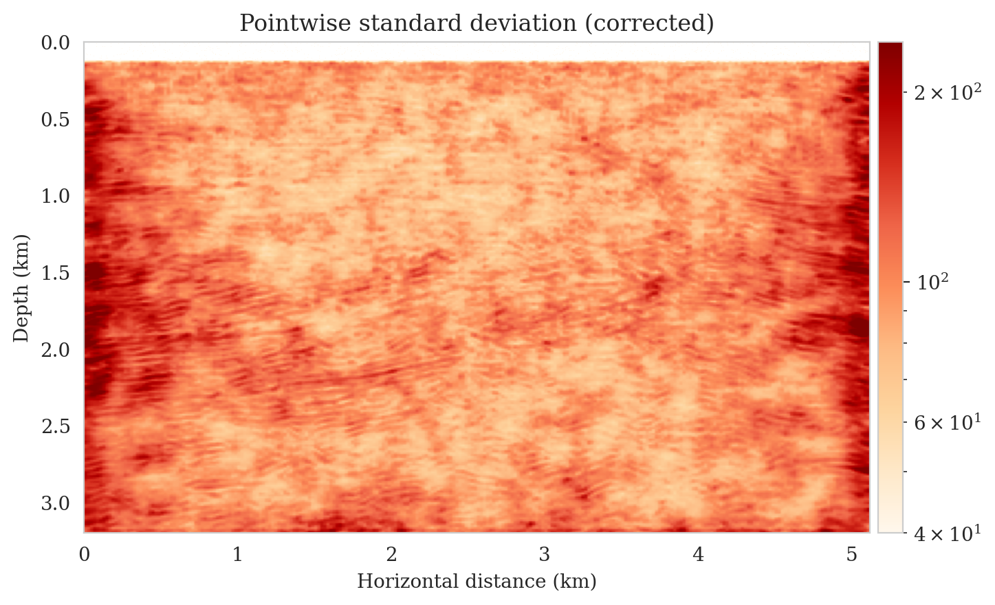
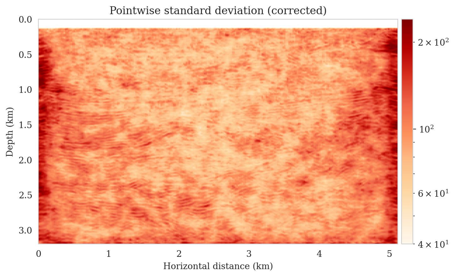
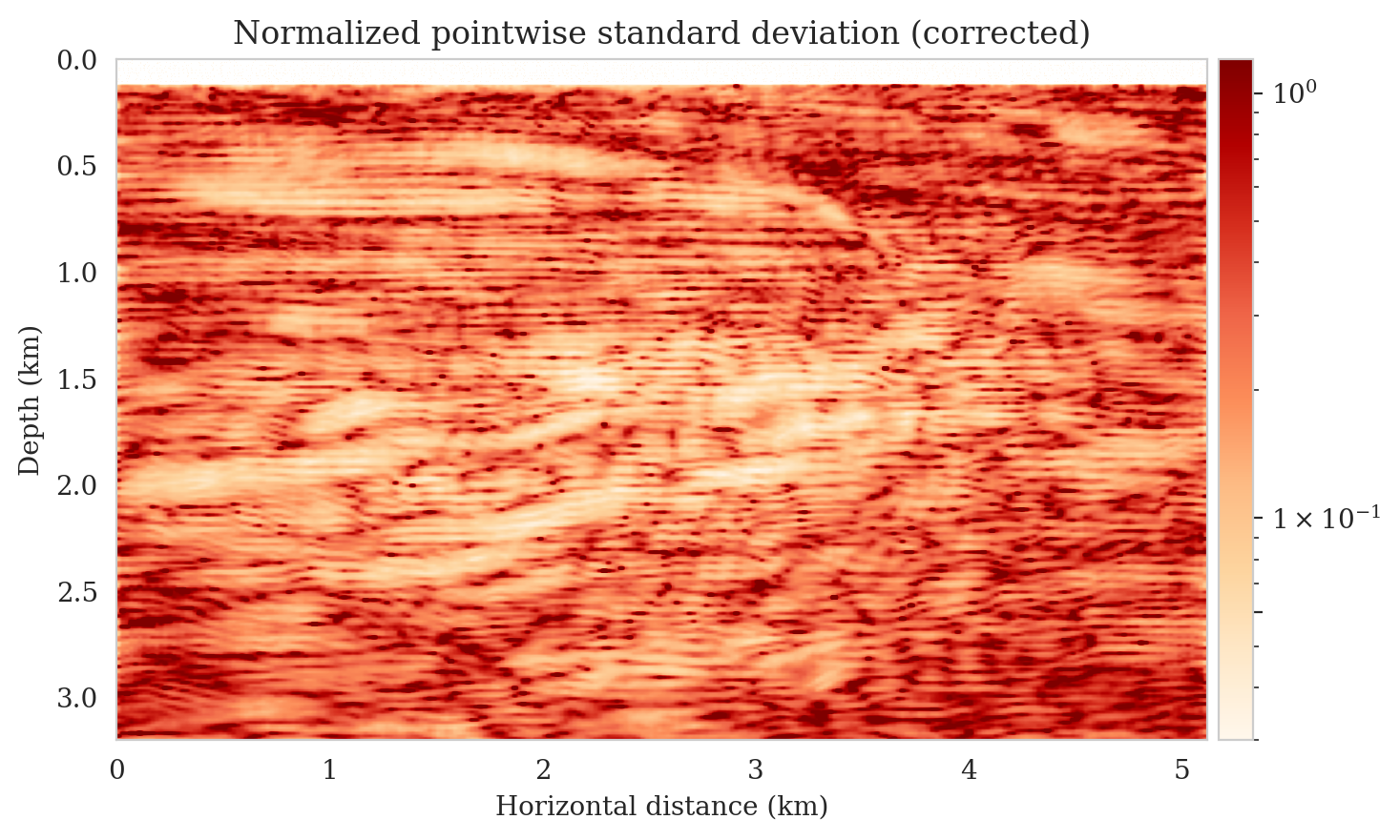
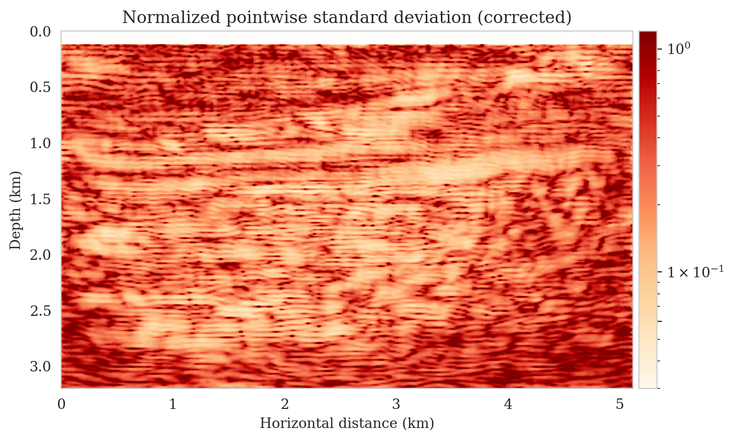
Data residuals

As before, we confirm that the latent distribution correction improves the fit of the data. Figure 24 shows the predicted data as well as the data residuals for all conditional mean estimates. The predicted data are obtained by applying the forward operator to the conditional mean estimates, both before and after latent distribution correction. The predicted data before and after correction are presented in the first and second columns, respectively. The corresponding data residuals before and after correction, which are computed by subtracting the predicted data from ideal noise-free data, can be seen in the third and last columns of Figure 24. Evidently, the latent distribution correction stage has resulted in a better fit with the observed data, as coherent data events show up in Figures 24c and 24g, but are attenuated in the corrected residual plots (Figures 24d and 24h).

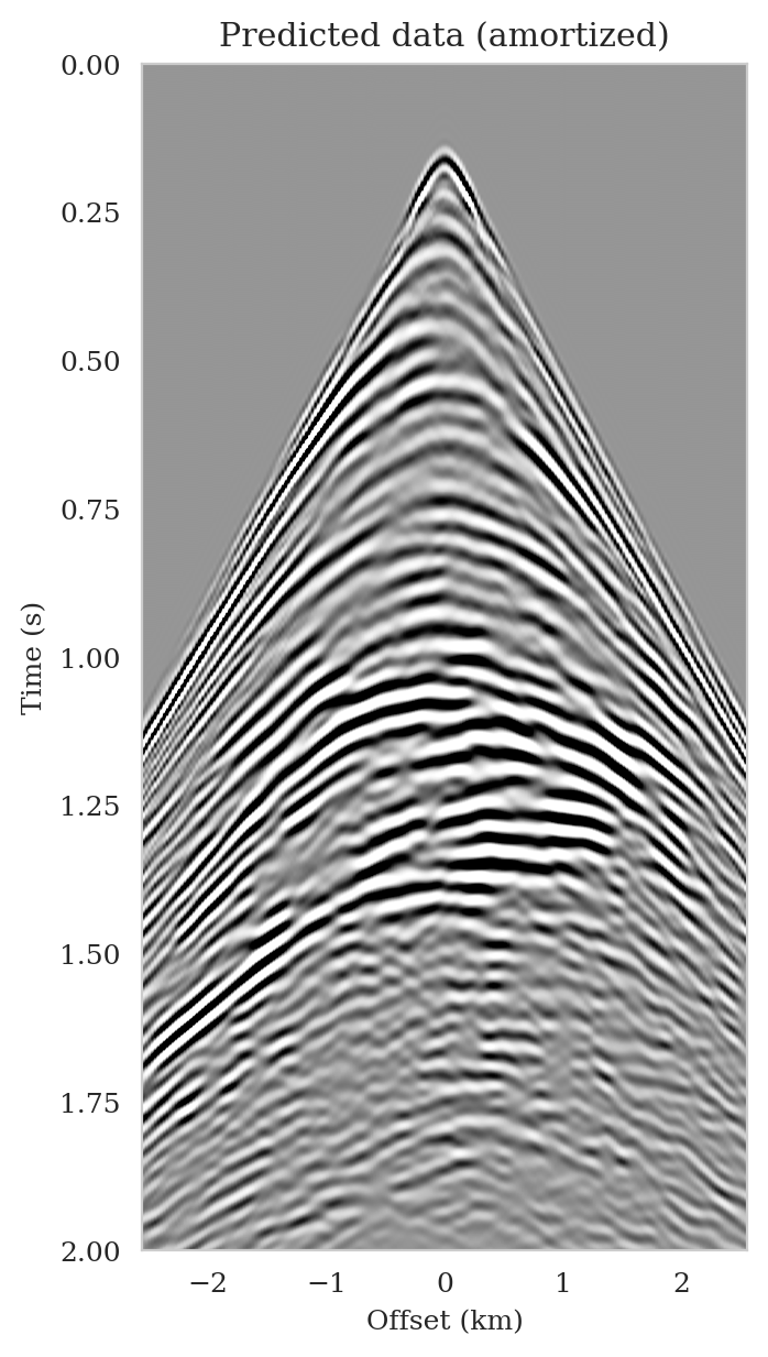
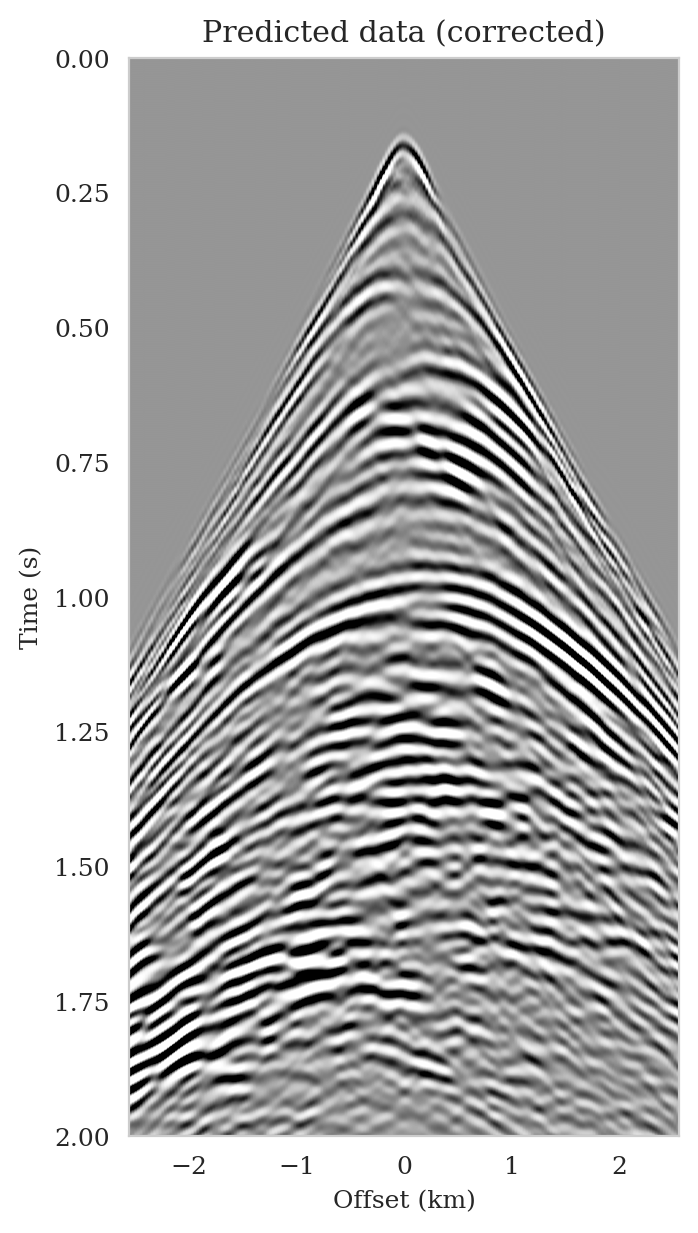
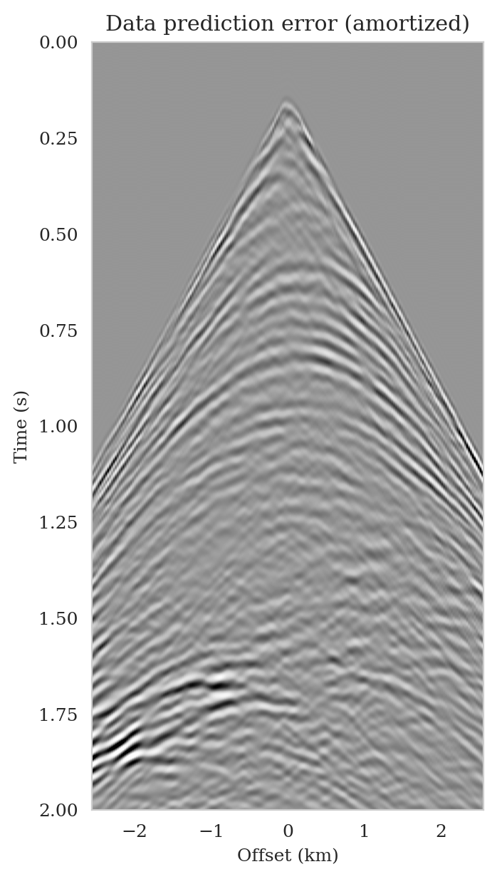
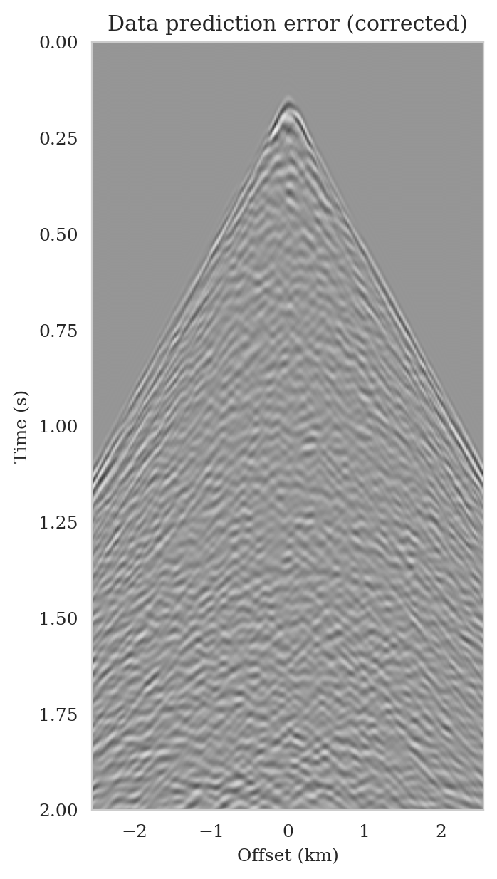
Discussion

The examples presented demonstrate that deep neural networks trained in the context of amortized variational inference can facilitate solving inverse problems in two ways: (1) incorporating prior knowledge gained through pretraining; and (2) accelerating Bayesian inference and uncertainty quantification. Despite the fact that amortized variational inference is capable of sampling the posterior distribution without requiring forward operator evaluations during inference, the extent to which it is considered reliable is dependent upon the availability of high quality training data. We demonstrate this limitation of amortized variational inference via a seismic imaging example where we alter the number of sources, variance of noise, and the present geological features to be imaged in comparison to the pretraining phase. These variations shift the data distribution, and in certain cases, e.g., imaging slightly different geological features, this can be also thought as evaluating the pretrained conditional normalizing flow over data samples from the low probability regions of the training distribution. Due to shifts in the data distribution, the obtained posterior samples via amortized variational inference in our numerical experiments had unusual near-source artifacts and less illuminated reflectors, which we can be partly attributed to lack of these artifacts in the training reverse-time migrated images.

As part of our efforts to extend the application of the supervised amortized variational inference methods to domains with limited access to high-quality training data, we developed an unsupervised, physics-based variational inference formulation over the latent space of a pretrained conditional normalizing flow that mitigates some of the posterior sampling errors induced by data distribution shifts. In this approach, a diagonal correction to the latent distribution is learned that ensures that the conditional normalizing flow output distribution better matches the desired posterior distribution. Based on observations and other research (Asim et al., 2020; Orozco et al., 2021; Siahkoohi et al., 2022b), we found that normalizing flows, because of their invertibility, are capable of partially mitigating errors related to changes in data distributions when they are used to solve inverse problems. We leave the delineation of which data distribution shifts can be handled by our diagonal correction approach to future work. Needless to say, by adhering to more complex transformations in the latent space, e.g., via a neural network, a wide range of data distribution shifts can be handled but it would potentially require a more computationally costly correction step.

Latent distribution correction requires several passes over the data (five in our example), which includes evaluation of the forward operator and the adjoint of its Jacobian. Due to the amortized nature of our approach, these costs are significantly lower than those incurred by other non-amortized variational inference methods (Rizzuti et al., 2020; Andrle et al., 2021; X. Zhang and Curtis, 2021; Zhao et al., 2022), specifically tens of thousands of forward operator evaluations reported by Zhao et al. (2021) in the context of travel-time tomography. By amortizing over the data, the pretrained conditional normalizing flow provides posterior samples for previously unseen data (drawn from the same distribution as training data) without the need for latent distribution correction. In presence of moderate data distribution shifts, the learned posterior is adjusted to new observed data via the latent distribution correction step, which could be considered an instance of transfer learning (Yosinski et al., 2014). In contrast, existing methods that perform variational inference in the latent space (Whang et al., 2021; Kothari et al., 2021) require a more substantial modification to the latent distribution, as the pretrained model in these methods originally provides samples from the prior distribution. For large-scale inverse problems, such as seismic imaging, where solving a partial differential equation is required to evaluate the forward operator, reduced computational costs of Bayesian inference are particularly important. Our approach reduces the computational costs associated with Bayesian inference in such problems while also complementing the inversion with a learned prior. In order to quantify the extent to which a diagonal correction to the latent distribution mitigates errors resulting from data distribution shifts, more research is required.

While the examples we presented in this paper were in regards to linear inverse problem, variational inference can be also applied to nonlinear problems (X. Zhang and Curtis, 2020, 2021; X. Zhang et al., 2021, 2022; D. Li, 2022). However, in the context of amortized variational inference there are two main considerations that need to be taken into account when dealing with large-scale nonlinear inverse problems. First, the parametric surrogate (conditional) distribution should be capable of approximating multi-modal densities. Invertible neural networks (Dinh et al., 2016) are a suitable choice for this parameterization as they are known to be universal approximators (Teshima et al., 2020; Ishikawa et al., 2022), meaning that invertible networks are capable of approximating a general class of diffeomorphisms. In other words, as long as there is a smooth invertible map between the latent space and the desired posterior distribution, invertible neural networks can be used to approximate the posterior distribution. The second consideration is regarding finding low-dimensional summary statistics (S. T. Radev et al., 2022) of observed data to avoid training the conditional normalizing flow over high dimensional data. In our linear seismic imaging example, we “summarized” seismic data (shot records) via the reverse-time migrated image. The conditions for which this summarization does not negatively bias the outcome of Bayesian inference (in the context of linear inverse problems) is described by Orozco et al. (2023). Further work is needed to design low-dimensional summary statistics for nonlinear inverse problems in order to successfully apply our framework to large-scale nonlinear inverse problems.

As far as seismic imaging is concerned, uncertainty can be attributed to two main sources (Thore et al., 2002; Osypov et al., 2013; G. Ely et al., 2018): (1) data errors, including measurement noise; (2) modeling errors, including linearization errors, which diminish with the accuracy of the background velocity model. The scope of our research is focused on the first source of uncertainty, and we will explore how variational inference models can be used to capture errors in background models in future work. In contrast to the problem highlighted in this paper, capturing the uncertainty caused by errors in the background model would require generating training data involving imaging experiments for a variety of plausible background velocity models, which would be computationally intensive. Recent developments in Fourier neural operators (Z. Li et al., 2021; Siahkoohi et al., 2022a) may prove to be useful in addressing this problem.

Conclusions

In high-dimensional inverse problems with computationally expensive forward modeling operators, Bayesian inference is challenging due to the cost of sampling the high-dimensional posterior distribution. The computational costs associated with the forward operator often limit the applicability of sampling the posterior distribution with traditional Markov chain Monte Carlo and variational inference methods. Added to the computational challenges are the difficulties associated with selecting a prior distribution that encodes our prior knowledge while not negatively biasing the outcome of Bayesian inference. Amortized variational inference addresses these challenges by incurring an offline initial training cost for a deep neural network that can approximate the posterior distribution for previously unseen observed data, distributed according to the training data distribution. When high-quality training data is readily available, and as long as there are no shifts in the data distribution, the pretrained network is capable of providing samples from the posterior distribution for previously unknown data virtually free of additional costs.

Unfortunately, in certain domains, such as geophysical inverse problems, where the structure of the Earth’s subsurface is unknown, it can be challenging to obtain a training dataset, e.g., a collection of images of the subsurface, which statistically captures the strong heterogeneity exhibited by the Earth’s subsurface. Furthermore, changes to the data generation process could negatively influence the quality of Bayesian inferences with amortized variational inferences due to generalization errors associated with neural networks. To address these challenges while exploiting the computational benefits of amortized variational inference, we proposed a data-specific, physics-based, and computationally cheap correction to the latent distribution of a conditional normalizing flow, pretrained to via an amortized variational inference objective. This correction involves solving a variational inference problem in the latent space of the pretrained conditional normalizing flow where we obtain a diagonal correction to the latent distribution such that the predicted posterior distribution more closely matches the desired posterior distribution.

Using a seismic imaging example, we demonstrate that the proposed latent distribution correction, at a cost of five reverse-time migrations, can be used to mitigate the effects of data distribution shifts, which includes changes in the forward model as well as the prior distribution. Our evaluation indicated improvements in seismic image quality, comparable to least squares imaging, after the latent distribution correction step, as well as estimate on the uncertainty of the image. We presented the pointwise standard deviation as a measure of uncertainty in the image, which indicated an increase in variability in complex geological areas and poorly illuminated areas. This approach will enable uncertainty quantification in large-scale inverse problems, which otherwise would be computationally expensive to achieve.

Related material

The latent distribution correction optimization problem (equation \(\ref{reverse_kl_covariance_diagonal}\)) involves computing gradients of the composition of the forward operator and the pretrained conditional normalizing flow with respect to the latent variable. Computing this gradient requires actions of the forward operator and the adjoint of its Jacobian. In our numerical experiments, these operations involved solving wave equations. For maximal numerical performance, we use JUDI (Witte et al., 2019) to construct wave-equation solvers, which utilizes the just-in-time Devito (Luporini et al., 2018; M. Louboutin et al., 2019) compiler for the wave-equation based simulations. The invertible network architectures are implemented using InvertibleNetworks.jl (Witte et al., 2021), a memory-efficient framework for training invertible nets in Julia programming language. For more details on our implementation, please refer to our code at https://github.com/slimgroup/ReliableAVI.jl.

Acknowledgments

This research was carried out with the support of Georgia Research Alliance and partners of the ML4Seismic Center.

Appendix A

Derivation of latent distribution correction objective function

The optimization problem for correcting the latent distribution involves minimizing the KL divergence between the Gaussian relaxation of the latent distribution \(\mathrm{N} \big(\B{z} \mid \Bs{\mu}, \operatorname{diag}(\B{s})^2\big)\) and the shifted latent distribution \(p_{\phi} (\B{z} \mid \B{y}_{\text{obs}})\), which is conditioned on an instance of out-of-distribution data \(\B{y}_{\text{obs}} \sim \widehat{p}_{\text{data}} (\B{y})\). This is an instance of non-amortized variational inference (see equations \(\ref{reverse_kl_divergence}\) and \(\ref{vi_reverse_kl}\)) defined over the latent variable: \[ \begin{equation} \begin{aligned} & \argmin_{\Bs{\mu}, \B{s}}\, \KL\,\big(\mathrm{N} \big(\B{z} \mid \Bs{\mu}, \operatorname{diag}(\B{s})^2\big) \mid\mid p_{\phi} (\B{z} \mid \B{y}_{\text{obs}}) \big) \\ & = \argmin_{\Bs{\mu}, \B{s}}\, \mathbb{E}_{\B{z} \sim \mathrm{N} (\B{z} \mid \Bs{\mu}, \operatorname{diag}(\B{s})^2)} \bigg [ -\log p_{\phi} (\B{z} \mid \B{y}_{\text{obs}}) + \log \mathrm{N} \big(\B{z} \mid \Bs{\mu}, \operatorname{diag}(\B{s})^2\big) \bigg ]. \end{aligned} \label{reverse_kl_covariance_diagonal_derivation} \end{equation} \] The above expression can be further simplified by rewriting the expectation with respect to \(\mathrm{N} \big(\B{z} \mid \Bs{\mu}, \operatorname{diag}(\B{s})^2\big)\) as the expectation with respect to a standard Gaussian distribution, followed by an elementwise scaling by \(\B{s}\) and a shift by \(\Bs{\mu}\) (see reparameterization trick in Diederik P. Kingma and Welling, 2014), i.e., \[ \begin{equation} \argmin_{\Bs{\mu}, \B{s}}\, \mathbb{E}_{\B{z} \sim \mathrm{N} (\B{z} \mid \B{0}, \B{I})} \bigg [ -\log p_{\phi} (\B{s} \odot\B{z} + \Bs{\mu} \mid \B{y}_{\text{obs}}) + \log \mathrm{N} \big(\B{s} \odot\B{z} + \Bs{\mu} \mid \Bs{\mu}, \operatorname{diag}(\B{s})^2\big) \bigg ]. \label{change-expectation} \end{equation} \] The last term in the expectation in equation \(\ref{change-expectation}\) is the log-density of a Gaussian distribution, which is equal to: \[ \begin{equation} \begin{aligned} & \log \mathrm{N} \big(\B{s} \odot\B{z} + \Bs{\mu} \mid \Bs{\mu}, \operatorname{diag}(\B{s})^2\big) \\ & = -\frac{D}{2} \log (2 \pi) -\frac{1}{2} \log \Big | \det \operatorname{diag}(\B{s})^2 \Big | -\frac{1}{2} \big(\B{s} \odot\B{z} + \Bs{\mu} -\Bs{\mu} \big)^{\top} \operatorname{diag}(\B{s})^{-2} \big(\B{s} \odot\B{z} + \Bs{\mu} -\Bs{\mu} \big) \\ & = - \log \Big | \det \operatorname{diag}(\B{s}) \Big | -\frac{1}{2} \big\| \B{z} \big\|_2^2 + \text{const} \\ & = - \log \Big | \det \operatorname{diag}(\B{s}) \Big | + \text{const}. \end{aligned} \label{gaussian_density} \end{equation} \] In the above equation, \(D\) is the dimension of \(\B{z}\), and the constants represent terms that are not a function of \(\Bs{\mu}\) or \(\B{s}\). By inserting equation \(\ref{gaussian_density}\) into equation \(\ref{change-expectation}\) we arrive at the following objective function for the latent distribution correction: \[ \begin{equation} \begin{split} \argmin_{\Bs{\mu}, \B{s}}\, \mathbb{E}_{\B{z} \sim \mathrm{N} (\B{z} \mid \B{0}, \B{I} )} \bigg [ -\log p_{\phi} (\B{s} \odot\B{z} + \Bs{\mu} \mid \B{y}_{\text{obs}}) - \log \Big | \det \operatorname{diag}(\B{s}) \Big | \bigg ] \\ \end{split} \label{reverse_kl_covariance_diagonal_final} \end{equation} \] Finally, we use use Bayes’ rule and inserting the shifted latent density function from equation \(\ref{physics_informed_density}\) to arrive at the objective function for latent distribution correction (equation \(\ref{reverse_kl_covariance_diagonal}\)): \[ \begin{equation} \begin{aligned} \argmin_{\Bs{\mu}, \B{s}} \mathbb{E}_{\B{z} \sim \mathrm{N} (\B{z} \mid \B{0}, \B{I})} \bigg [& \frac{1}{2 \sigma^2} \sum_{i=1}^{N} \big \| \B{y}_{\text{obs}, i}-\mathcal{F}_i \circ f_ {\phi} \big(\B{s} \odot\B{z} + \Bs{\mu}; \B{y}_{\text{obs}} \big) \big\|_2^2 \\ & + \frac{1}{2} \big\| \B{s} \odot \B{z} + \Bs{\mu} \big\|_2^2 - \log \Big | \det \operatorname{diag}(\B{s}) \Big | \bigg ]. \end{aligned} \label{reverse_kl_covariance_diagonal-derived} \end{equation} \]