Adjoint operators enable fast and amortized machine learning based Bayesian uncertainty quantification

ABSTRACT:

Machine learning algorithms such as Normalizing Flows, VAEs, and GANs are powerful tools in Bayesian uncertainty quantification (UQ) of inverse problems. Unfortunately, when using these algorithms medical imaging practitioners are faced with the challenging task of manually defining neural networks that can handle complicated inputs such as acoustic data. This task needs to be replicated for different receiver types or configurations since these change the dimensionality of the input. We propose to first transform the data using the adjoint operator —ex: time reversal in photoacoustic imaging (PAI) or back-projection in computer tomography (CT) imaging — then continue posterior inference using the adjoint data as an input now that it has been standardized to the size of the unknown model. This adjoint preprocessing technique has been used in previous works but with minimal discussion on if it is biased. In this work, we prove that conditioning on adjoint data is unbiased for a certain class of inverse problems. We then demonstrate with two medical imaging examples (PAI and CT) that adjoints enable two things: Firstly, adjoints partially undo the physics of the forward operator resulting in faster convergence of an ML based Bayesian UQ technique. Secondly, the algorithm is now robust to changes in the observed data caused by differing transducer subsampling in PAI and number of angles in CT. Our adjoint-based Bayesian inference method results in point estimates that are faster to compute than traditional baselines and show higher SSIM metrics, while also providing validated UQ.

STATEMENT OF PURPOSE:

The efficiency and power of machine learning methods have accelerated the development in inverse problems of a variety of fields (Ongie et al., 2020). Unfortunately, many machine learning methods are black boxes with failure cases that are difficult to interpret. This is one of the reasons that their adoption in safety critical settings is hampered. Our purpose is to improve machine learning (ML) for medical imaging by enabling uncertainty that is amortized. This is important since applying ML under distribution shifts or poor training can cause instabilities and even hallucinations leading to incorrect diagnoses (Antun et al., 2020, Bhadra et al. (2021)). Uncertainty quantification (UQ) aims to aid this problem by communicating to practitioners when a model is confident in its result versus when it should not be trusted. We describe a practical UQ framework based on amortized variational inference (AVI) and adjoint operators. These two concepts marry powerful data-driven methods with physics knowledge allowing us to amortize over unseen data and also different imaging configurations. By amortizing, we mean that the framework generalizes over new data.

The particular class of algorithms we study, can be trained given only examples of the parameters of interest \(\mathbf{x}\) and their corresponding simulated data \(\mathbf{y}\). In medical imaging, data \(\mathbf{y}\) can contain complex physical phenomena such as acoustic waves in photoacoustic imaging. To a certain extent, an ML-based algorithm learns to \(\mathit{undo}\) the complex physical phenomena when providing an estimate of \(\mathbf{x}\). This can lead to long training times which we would like to ameliorate. We are also interested in creating an algorithm that is robust to changes in the dimensionality of the observations \(\mathbf{y}\) caused by changes in the imaging configuration such as changing the number of transducers. To solve both problems, we propose preprocessing the data \(\mathbf{y}\) with the adjoint operator.

We first show that the posterior given data is equivalent to the posterior given data preprocessed with the adjoint in the case of linear forward operators and Gaussian noise. Many medical imaging modalities fall in this category: Photoacoustic imaging, CT and MRI. Equipped with this theoretical result, we demonstrate two practical advantages of adjoint preprocessing. First, it accelerates training convergence of AVI with conditional normalizing flows. This is a welcome result since normalizing flows are notoriously costly to train (40 GPU weeks for the seminal GLOW normalizing flow (Kingma and Dhariwal, 2018)). Second, the adjoint brings data to the model space and therefore standardizes data size, enabling us to learn a single amortized neural network that can sample the posterior for a variety of imaging configurations. We demonstrate these results using two medical imaging applications. These contributions fulfill our stated purpose by describing a practical UQ framework that has a theoretical basis.

METHODS:

Bayesian Uncertainty Quantification of Inverse Problems:

At the forefront of uncertainty quantification (UQ) for inverse problems are Bayesian methods(Tarantola, 2005). First, we setup a forward problem. Given our quantity of interest \(\mathbf{x} \in \mathcal{X}\) called the model, the forward problem is described by a linear operator \(\mathbf{A}: \mathcal{X} \rightarrow \mathcal{Y}\) whose action on \(\mathbf{x}\) gives observations \(\mathbf{y} \in \mathcal{Y}\). Here, we consider linear problems with additive Gaussian noise term \(\pmb\varepsilon\)—i.e., \[ \begin{equation} \mathbf{y} = \mathbf{A}\mathbf{x} + \pmb\varepsilon. \label{eq:forward} \end{equation} \] Upon observing data \(\mathbf{y}\), traditional methods in inverse problems create a single point estimate of the \(\mathbf{x}\) that produced \(\mathbf{y}\).
In the absence of noise and for invertible operators this point estimate is enough to describe the solution of the inverse problem. This approach fails to fully characterize the solution space in ill-posed problems (Hadamard, 1902), where there is no guarantee of a unique solution. In a Bayesian framework, we instead try to find the set or of solutions that all explain the data. This set of solutions is encoded by the conditional distribution \(\mathbf{x}\sim p(\mathbf{x}\mid \mathbf{y})\) called the posterior distribution and is the end goal of Bayesian inference . It contains all information needed to estimate \(\mathbf{x}\) given \(\mathbf{y}\) while providing UQ. Calculating the posterior distribution can be done with two main type of algorithms: first, sampling based algorithms such as Markov chain Monte Carlo (MCMC) algorithms (Robert et al., 1999) and second, optimization based algorithms such as variational inference (VI) (Blei et al., 2017). MCMC can be a costly method due to amount of sampling required (Gelman et al., 1995), especially in high-dimensional problems. We explore variational inference (VI) (Blei et al., 2017) to efficiently sample the posterior.

Variational Inference for Posterior Distribution Learning:

Our goal is to calculate a distribution so our problem is essentially density estimation of the posterior distribution. VI methods (Blei et al., 2017) turn the problem of density estimation by finding a parameterized distribution that best fits the desired distribution. The goodness of fit is typically measured by the Kullback-Leibler (KL) divergence. Among the various VI methods for density estimation, normalizing flows (Dinh et al., 2016) have been shown to be flexible, efficient and powerful while working on a variety of distributions including conditional distributions (Kingma and Dhariwal, 2018, Ardizzone et al. (2018)). For our case, the goal is to find the normalizing flow \(f_{\theta}\) parameterized by \(\theta\) that makes a learned conditional distribution \(p_{\theta}(\mathbf{x}\mid \mathbf{y})\) approximate the desired posterior distribution \(p(\mathbf{x}\mid \mathbf{y})\). We measure the goodness-of-fit with the KL-divergence making our optimization objective \[ \begin{equation} \hat\theta = \underset{\mathbf{\theta} }{\operatorname{arg \, min}} \, \mathbb{KL}\, ( \, p_{\theta}(\mathbf{x}\mid \mathbf{y}) \, \,||\,\, p(\mathbf{x}\mid \mathbf{y}) ). \label{eq:KL} \end{equation} \] Previous work has been put into VI with normalizing flows that involves costly optimization for each incoming observed data \(\mathbf{y}\) (Whang et al., 2021, H. Sun and Bouman (2020), Rizzuti et al. (2020), Zhao et al. (2022)). The optimization is costly because learned parameters of \(f_{\theta}\) typically parameterize neural networks that are costly to optimize. On top of that, these VI objectives requires online use of the forward operator \(\mathbf{A}\) and its adjoint \(\mathbf{A}^{\ast}\) during optimization. With this formulation, VI is not efficient enough to enable real-time inference. Real-time results are particularly important in medical imaging settings since they extend the abilities of a given modality for example by enabling the use of hand-held probes (Dima and Ntziachristos, 2012, buehler2013real). In general, minimizing turnover time makes the difference in providing a timely diagnosis (Bauer et al., 2013).

Amortized Variational Inference with Conditional Normalizing Flows:

A formulation of VI called amortized variational inference (AVI) (Kovachki et al., 2020,Kruse et al. (2019), Orozco et al. (2021), Siahkoohi et al. (2022a), Gershman and Goodman (2014)) aims to obtain fast inference on test data without having to re-optimize an objective. This is accomplished by optimizing a Kullbeck-Liebler (KL) divergence based objective that is \(\mathit{amortized}\) over different data \(\mathbf{y}\) sampled from the distribution \(p(\mathbf{y})\): \[ \begin{equation} \hat\theta = \operatorname{arg \,min}_{\theta} \, \mathbb{E}_{\mathbf{y} \sim {p(\mathbf{y})}} \left[ \mathbb{KL} \, ( p(\mathbf{x}\mid \mathbf{y}) \,||\, p_{\theta}(\mathbf{x}\mid \mathbf{y}) ) \right] . \label{eq:KLamort} \end{equation} \] In this form, the objective can not be implemented since it would require access to the ground truth posterior distribution \(p(\mathbf{x}\mid\mathbf{y})\). One can optimize a simplified objective that only requires samples from the joint distribution \(\mathbf{x},\mathbf{y} \sim p(\mathbf{x},\mathbf{y})\). For a conditional normalizing flow (CNF) \(f_{\theta}\), the AVI objective becomes \[ \begin{equation} \hat\theta = \underset{\theta}{\operatorname{arg \, min}} \, \frac{1}{N} \sum_{n=1}^{N} \left( \lVert f_{\theta}(\mathbf{x}^{(n)};\mathbf{y}^{(n)}) \rVert_{2}^2 - \log \left| \det{ \mathbf{J}_{f_{\theta}}} \right| \right) \label{eq:KLamortML} \end{equation} \] where \(N\) is the size of a training dataset and \(\mathbf{J}_{f_{\theta}}\) is the Jacobian of the CNF. This objective is derived in (Radev et al., 2020) and in (Siahkoohi et al., 2022b) with a discussion on its relationship to the forward and backward KL-divergence. This objective is particularly simple to implement with CNFs since they allow for tractable computation of the determinant Jacobian term \(\det{ \mathbf{J}_{f_{\theta}}}\) by design.

Our goal is to amortize our CNF for a variety of imaging configurations. Then we must consider that for a model \(\mathbf{x}\) of one size, a different imaging configuration \(i\) (here encoded into the forward operator as \(\mathbf{A_i}\)) can change the size of \(\mathbf{y_i}\). These different data sizes can arise from changing receiver settings such as number of receivers or view angles. To handle a set of imaging configurations \(\{i = 1:M\}\) (where \(M\) is the number configurations), one would need to define a network \(f_{\theta_i}\), for all \(M\) configurations i.e. manually defining downsampling layers. Standardizing observations to a single size would allow practitioners to only need to define a single network \(f_{\theta}\) since now all inputs to the network are the same size regardless of their imaging configurations. The adjoint \(\mathbf{A^{\ast}_i}\) offers a physically consistent way of standardizing data inputs to a single size, namely the size of the model.

Adjoint:

Given a linear operator \(\mathbf{A}\) that acts on inner product spaces \(\mathcal{X} \rightarrow \mathcal{Y}\). The adjoint \(\mathbf{A}^{\ast}: \mathcal{Y} \rightarrow \mathcal{X}\) is the operator that makes the following true for any \(\mathbf{x}\) and \(\mathbf{y}\): \(\langle \mathbf{y} , \mathbf{A}\mathbf{x} \rangle = \langle \mathbf{A}^{*}\mathbf{y}, \mathbf{x} \rangle.\)

Standardizing the size of incoming data is related to the concept of a summary statistic (Deans, 2002, radev2020bayesflow) so can we interpret the adjoint as a physics-based summary statistic. We will show that on top of being robust over different imaging configurations, adjoints also accelerate the convergence of the training objective in Equation \(\ref{eq:KLamortML}\)]. Before demonstrating these two practical advantages of using the adjoint, we present our main contribution: a theoretical discussion showing when preprocessing data with the adjoint will not affect the result of posterior inference.

Adjoint Preprocessing is Unbiased for Linear Problems with Gaussian Noise:

As noted in the previous section, there are good reasons to use the adjoint operator as a preprocessor. This leads to an important question: that we phrase using the language of (Baptista et al., 2022): can we condition on adjoint data without introducing bias into the inference procedure? We will answer this question in the affirmative. We use Proposition 1 from (Adler et al., 2022) and specify a class of inverse problems that satisfies the proposition with adjoint preprocessing.

Proposition 1:(Adler et al., 2022)

If \(\mathcal{B}\) is injective on the range of \(\Pi\) then \(p(\mathbf{x} \mid \mathcal{B}\,\Pi \, \mathbf{y} )\) will be equal to \(p(\mathbf{x} \mid \mathbf{y})\) if and only if the information lost by observing \(\Pi \mathbf{y}\) instead of \(\mathbf{y}\) is conditionally independent of \(\mathbf{x}\) given \(\Pi \mathbf{y}\): \[ \begin{equation} p(\mathbf{x} \mid \mathcal{B}\,\Pi \, \mathbf{y} ) = p(\mathbf{x} \mid \mathbf{y}) \iff \mathbf{x} \bigCI \mathbf{y} - \Pi \mathbf{y} \mid \Pi \mathbf{y}. \label{eq:prop1cond} \end{equation} \] #### Proposition 1a: Given data \(\mathbf{y}\) (created as in Equation \(\eqref{eq:forward}\)), the posterior conditioned on adjoint-preprocessed data \(p(\mathbf{x}\mid \mathbf{A}^{\ast}\mathbf{y})\) will be equal to the original posterior \(p(\mathbf{x}\mid \mathbf{y})\) if the additive noise is Gaussian.

We use Proposition 1 from(Adler et al., 2022) and set \(\mathcal{B}=\mathbf{A}^\ast\); and \(\Pi\) to be the orthogonal projector onto \(\mathrm{ran}(\mathbf{A})\); \(\Pi=\mathbf{A}\mathbf{A}^{+}\) where \(\mathbf{A}^{+}\) is the Moore-Penrose inverse. [Penrose (1955)}. Since \(p(\mathbf{x} \mid \mathcal{B} \, \Pi \mathbf{y} ) = p(\mathbf{x} \mid \mathbf{A}^{\ast} \mathbf{A} \mathbf{A}^{+} \mathbf{y} ) = p(\mathbf{x} \mid \mathbf{A}^{\ast} \mathbf{y} )\) then our proof is complete if we show that the following conditional independence in \(\eqref{eq:prop1cond}\) is true: \(\mathbf{x} \bigCI \mathbf{y} - \mathbf{A}\mathbf{A}^{+}\mathbf{y} \mid \mathbf{A}\mathbf{A}^{+}\mathbf{y}.\)

To show this, we note that Gaussian noise can be decomposed as the sum of two independent components – one that lives in \(\mathrm{ran}(\mathbf{A})\) (the range of \(\mathbf{A}\)) and another that lives in \(\mathrm{ran}(\mathbf{A}_{})^\perp\) : \(\pmb\varepsilon = \pmb\varepsilon_{\mathbf{ran }} + \pmb\varepsilon_{\perp}\).

Assuming this structure: \[ \begin{equation} \begin{split} \begin{array}{c} \,\,\mathbf{x} \bigCI \mathbf{\mathbf{y}} - \mathbf{A}\mathbf{A}^{+}\mathbf{y} \mid \mathbf{A}\mathbf{A}^{+}\mathbf{y} \nonumber\\ = \,\, \mathbf{x} \bigCI (\mathbf{A}\mathbf{x} + \pmb\varepsilon_{\mathbf{\perp}} + \pmb\varepsilon_{\mathbf{ran}}) - \mathbf{A}\mathbf{A}^{+}(\mathbf{A}\mathbf{x} + \pmb\varepsilon_{\mathbf{\perp}} + \pmb\varepsilon_{\mathbf{ran}}) \mid \mathbf{A}\mathbf{A}^{+}(\mathbf{A}\mathbf{x} + \pmb\varepsilon_{\mathbf{\perp}} + \pmb\varepsilon_{\mathbf{ran}}) \nonumber\\ = \,\, \mathbf{x} \bigCI \mathbf{A}\mathbf{x} + \pmb\varepsilon_{\mathbf{\perp}} + \pmb\varepsilon_{\mathbf{ran}} - \mathbf{A}\mathbf{A}^{+}\mathbf{A}\mathbf{x} - \pmb\varepsilon_{\mathbf{ran}} \mid \mathbf{A}\mathbf{A}^{+}\mathbf{A}\mathbf{x} + \pmb\varepsilon_{\mathbf{ran}} \nonumber\\ = \,\, \mathbf{x} \bigCI \pmb\varepsilon_{\perp} \mid \mathbf{A}\mathbf{x} + \pmb\varepsilon_{\mathbf{ran}}. \end{array} \end{split} \label{eq:derivation} \end{equation} \] By the d-separation criterion, (Pearl, 1988), the statement is true because \(\pmb\varepsilon_{\perp}\) is independent of all other elements, including \(\pmb\varepsilon_{\mathbf{ran}}\) as per the assumption. Thus we prove that for linear problems with Gaussian additive noise \(p(\mathbf{x} \mid \mathbf{A}^{\ast} \mathbf{y} ) = p(\mathbf{x} \mid \mathbf{y})\) meaning adjoint preprocessing does not change the result posterior inference.

Assuming Gaussian additive noise covers several medical imaging modalities including our applications in photoacoustic imaging and CT[Gravel et al. (2004)}. Apart from non-Gaussian noise, our proof does not cover multiplicative noise or noise correlated with \(\mathbf{A}\) or \(\mathbf{x}\). We leave those for future work.

RESULTS:

We show three main results. First, that adjoint preprocessing accelerates the convergence of a conditional normalizing flow training to sample from the posterior distribution. Secondly, we demonstrate that the adjoint operator enables amortization over varying imaging configurations while using the same underling neural network. Finally, we validate the learned UQ by demonstrating posterior consistency through three tests.

Adjoint Accelerates Convergence:

We motivate adjoint preprocessing by hand-crafting a photoacoustic simulation and CNF architecture to compare the two scenarios, namely learning \(p_{\theta}(\mathbf{x} \mid \mathbf{y})\) by training on pairs \(\mathbf{D}= \{ (\mathbf{x}^{(n)}, \mathbf{y}^{(n)}) \}_{n=1}^{N} \) or adjoint preprocessed learning of \(p_{\theta}(\mathbf{x} \mid \mathbf{A}^{\ast}\mathbf{y})\) with \(\mathbf{D^{\ast}}= \{ (\mathbf{x}^{(n)}, \mathbf{A}^\ast\mathbf{y}^{(n)}) \}_{n=1}^{N} \). s noted in our motivations, creating a CNF \(f_{\theta}\) that can accept raw data \(\mathbf{y}\) as an input is a laborious task but we do this for one imaging configuration to provide a fair comparison. This task involves defining a physical simulation and architecture that makes \(\mathbf{y} \in \mathbb{R}^{N_t \times N_{\mathrm{rec}}}\) (where \(N_t\) = number time steps and \(N_{\mathrm{rec}}\) = number of receivers) to have the same size as the model \(\mathbf{x} \in \mathbb{R}^{N_x\times N_y}\) (where (\(N_x\),\(N_y\)) is the 2D grid size). To accomplish this, we to set the number of receivers to be the same as the number of grid points on a side \(N_{\mathrm{rec}}=N_y\). This makes the raw data matrix \(\mathbf{y}\) have the same number of column as the model \(\mathbf{x}\). Then we include a learned downsampling layer \(d_{\theta}\) that takes the data matrix and downsamples the number of rows to the number of grid points in the other side \(N_x\): \(d_{\theta}(\mathbf{y}) = \hat{\mathbf{y}} \in \mathbb{R}^{N_x\times N_y}\). Then we can proceed to train two CNF’s where both underlying networks have the same architectures and are trained using the same hyperparameters.

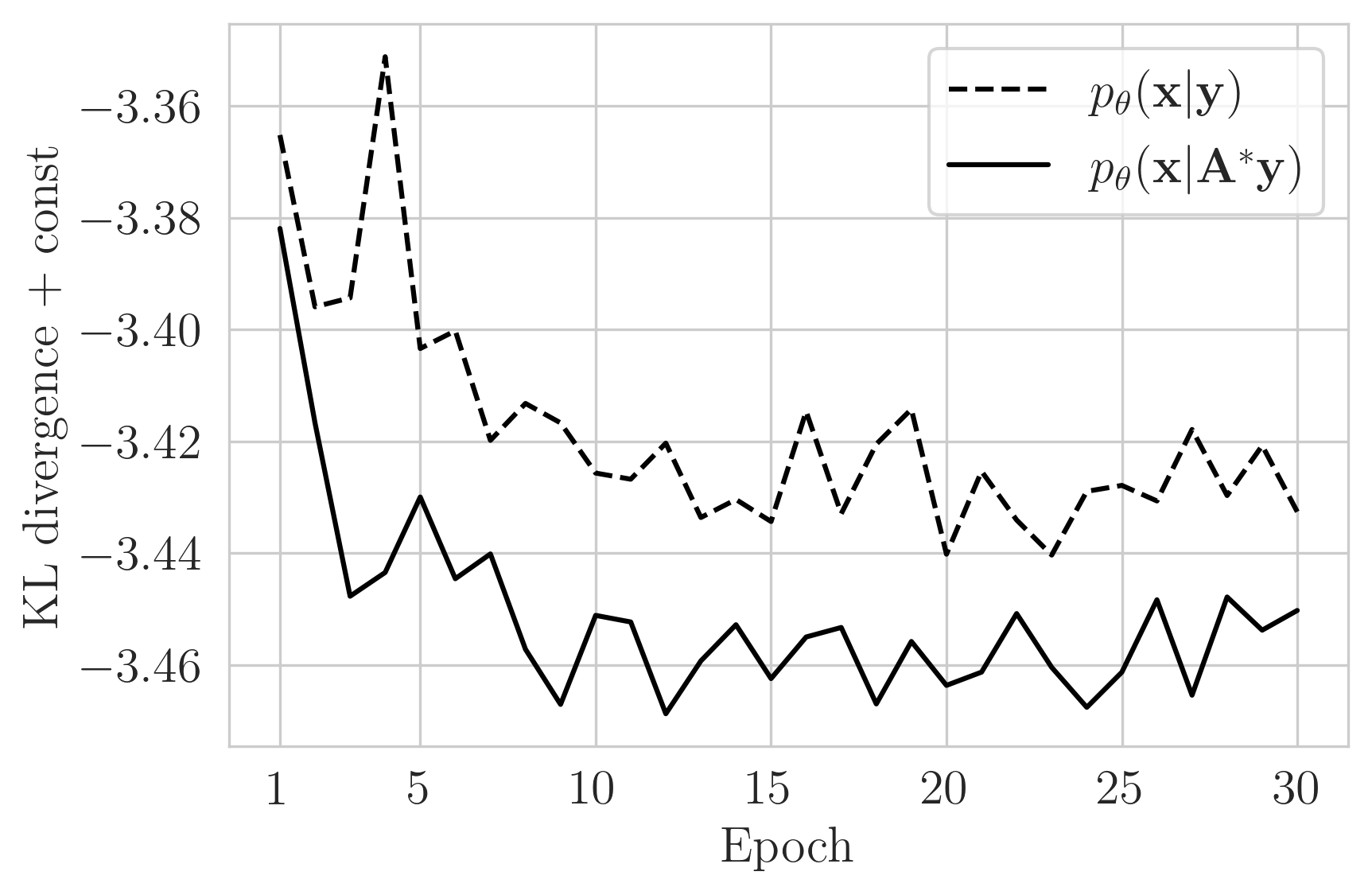
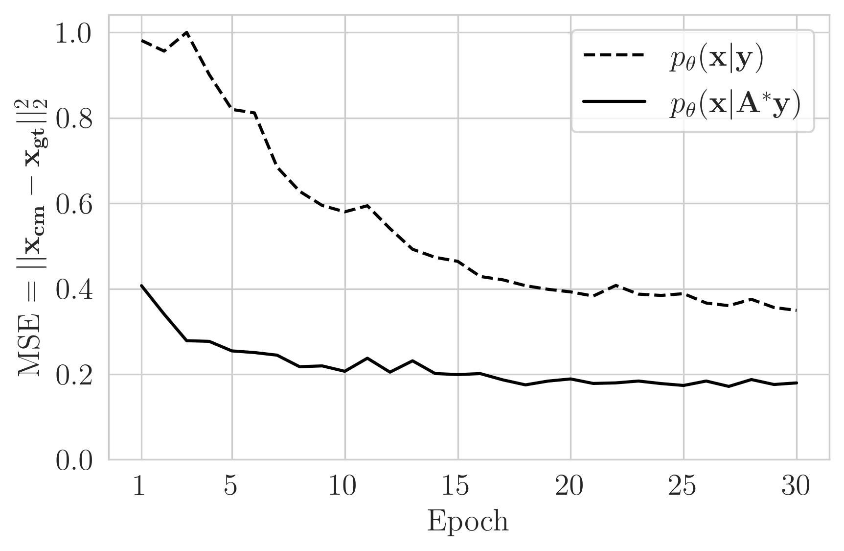
Figure 1 shows that for equivalent architectures and training, learning \(p_{\theta}(\mathbf{x}|\mathbf{A}^{\ast}\mathbf{y})\) is accelerated compared to learning \(p_{\theta}(\mathbf{x}|\mathbf{y})\). We also plot the mean squared error (MSE) between the calculated conditional mean \(\mathbf{x_{cm}}\) and the ground truth \(\mathbf{x_{gt}}\). While MSE is not the training objective, it is still an important proxy since the conditional mean of the true posterior is the one that gives the lowest expected error (Banerjee et al., 2005, Adler and Öktem (2018)). Here and throughout, the conditional mean is estimated from 64 generated samples of the posterior. The training logs in Figure 1 are averages of an unseen validation set \(N_{\mathrm{val}}\)=192 created by a 10% split from the training dataset of \(N\)=2048 pairs.

Adjoint Amortizes Different Imaging Configurations:

Preprocessing observed data with the adjoint allows us to use the same network to learn the posterior for different imaging configurations. As proof of concept, we amortize over four photoacoustic imaging configurations consisting of data collected with 8, 16, 32, and 64 receivers. These different configurations are encoded by forward and adjoint operators \(\mathbf{A_{i}},\mathbf{A^{\ast}_{i}}\) with \(i\in\{8,16,32,64\}\). We train our CNF with \(N\)=2048 examples for each imaging configuration \(\mathbf{D}_{\mathbf{i}}^{\ast}= \{ (\mathbf{x}^{(n)}, \mathbf{A_i^\ast}\mathbf{y_i}^{(n)}) \}_{n=1}^{N} \). Training took 14 hours on P1000 4GB GPU.

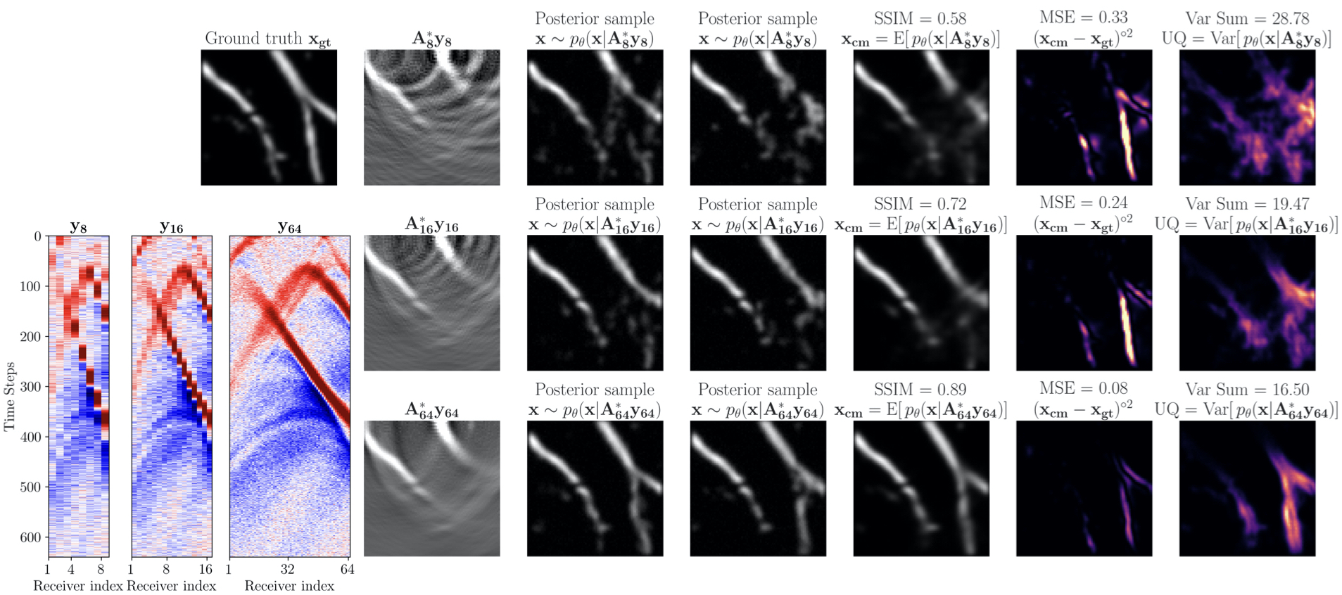
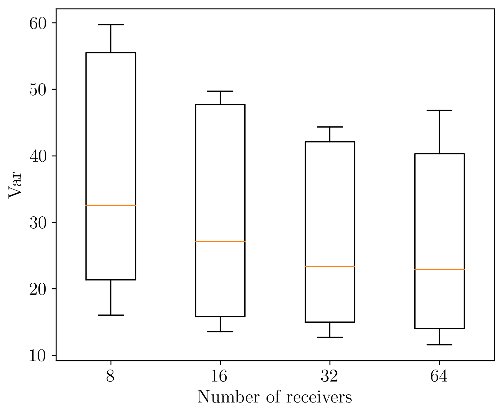
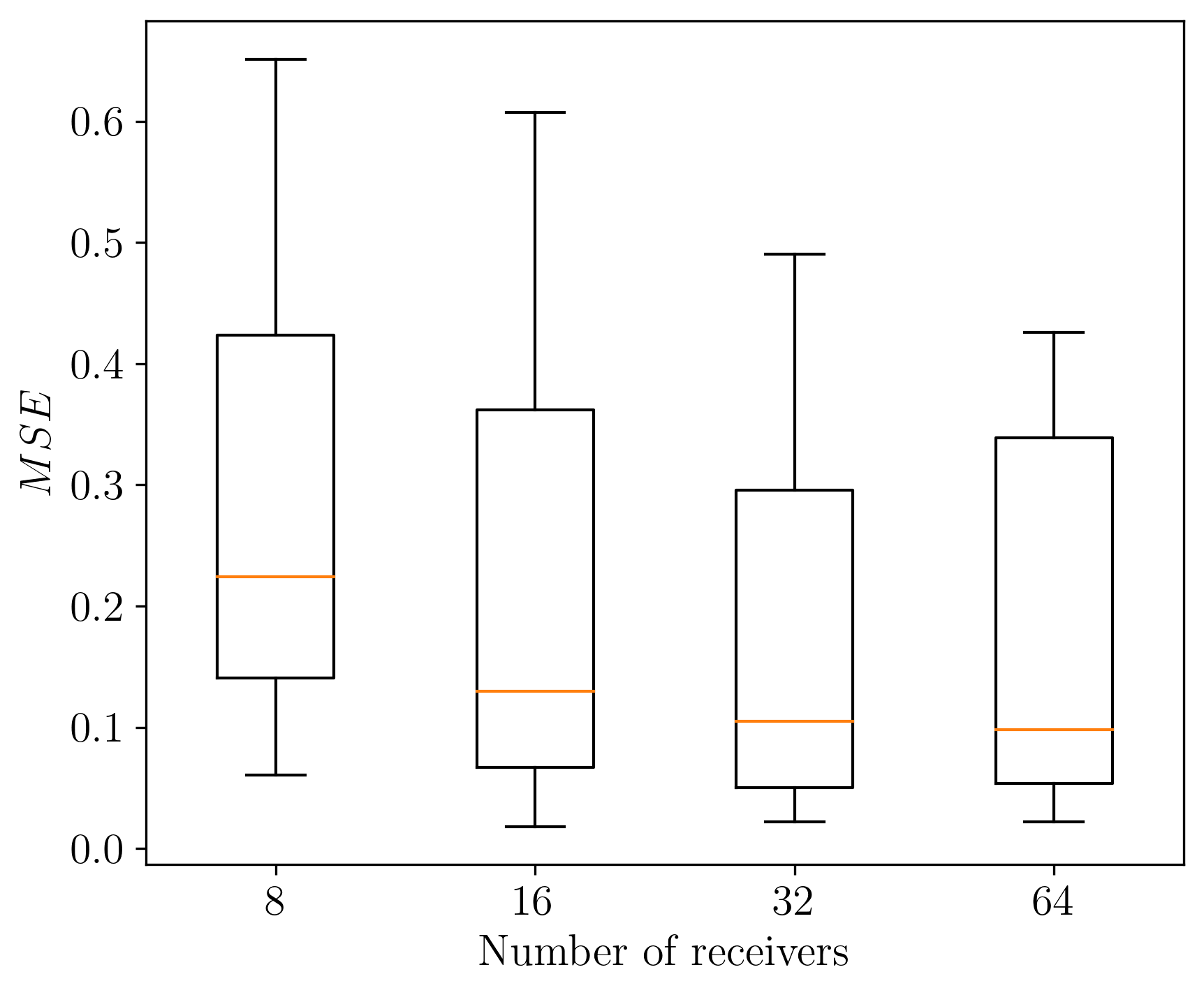
After training, we sample from the learned posterior for unseen test data examples, \(\mathbf{y_i}\) for varying numbers of receivers. As expected, we observe posterior contraction[Ghosal and Van der Vaart (2017)}. Visually, this is confirmed in Figure 2a since uncertainty (quantified via pointwise variance) goes down when we increase receivers from 16 to 64. To quantitatively capture the global variation of these UQ images, we use the sum of pointwise variances: Var Sum = \(\left|\mathrm{Var}\right|_1\). or equivalently the trace of the covariance matrix [Oja (1999)}. Importantly, uncertainty is high where we expect, namely for vessels that are close to being vertical. These vertical events are in the null-space of the forward operator because the receivers are only located at the top of the model.

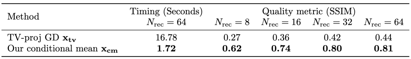
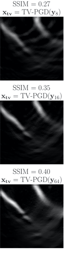
We emphasize that our posterior sampling after training is fast. The computational cost is dominated by the single adjoint (0.8 sec on Intel Skylake CPU). The CNF is conditioned on \(\mathbf{A^\ast_i}\mathbf{y_i}\) then the user generates the desired quantity of posterior samples (10 millisec/sample on our GPU). The time to create a point estimate with the conditional mean \(\mathbf{x_{cm}}\) (2 seconds with 64 posterior samples) is favorable compared to traditional least-squares approaches that require several forward and adjoint evaluations. We compare our point estimate \(\mathbf{x_{cm}}\) with TV-projected gradient descent (TV-PGD) [Y. Zhang et al. (2012), Schwab et al. (2018)} \(\mathbf{x_{tv}}\). Timing and quality metrics averaged over a test set of 96 samples are in Figure 3. We show better SSIM quality while producing our point estimate in less time. .

Validation of Uncertainty Quantification:

Since our problem does not have Gaussian priors, we can not analytically verify that our converged posteriors have reached the ground truth posterior. For validation purposes, we conduct three tests, namely via

\(\textit{(i) posterior contraction}\) by testing the CNF for different data sizes to check whether the posterior demonstrates contraction to the ground truth when increasing the amount of observed data. This contraction ultimately points to posterior consistency (Ghosal and Van der Vaart, 2017);

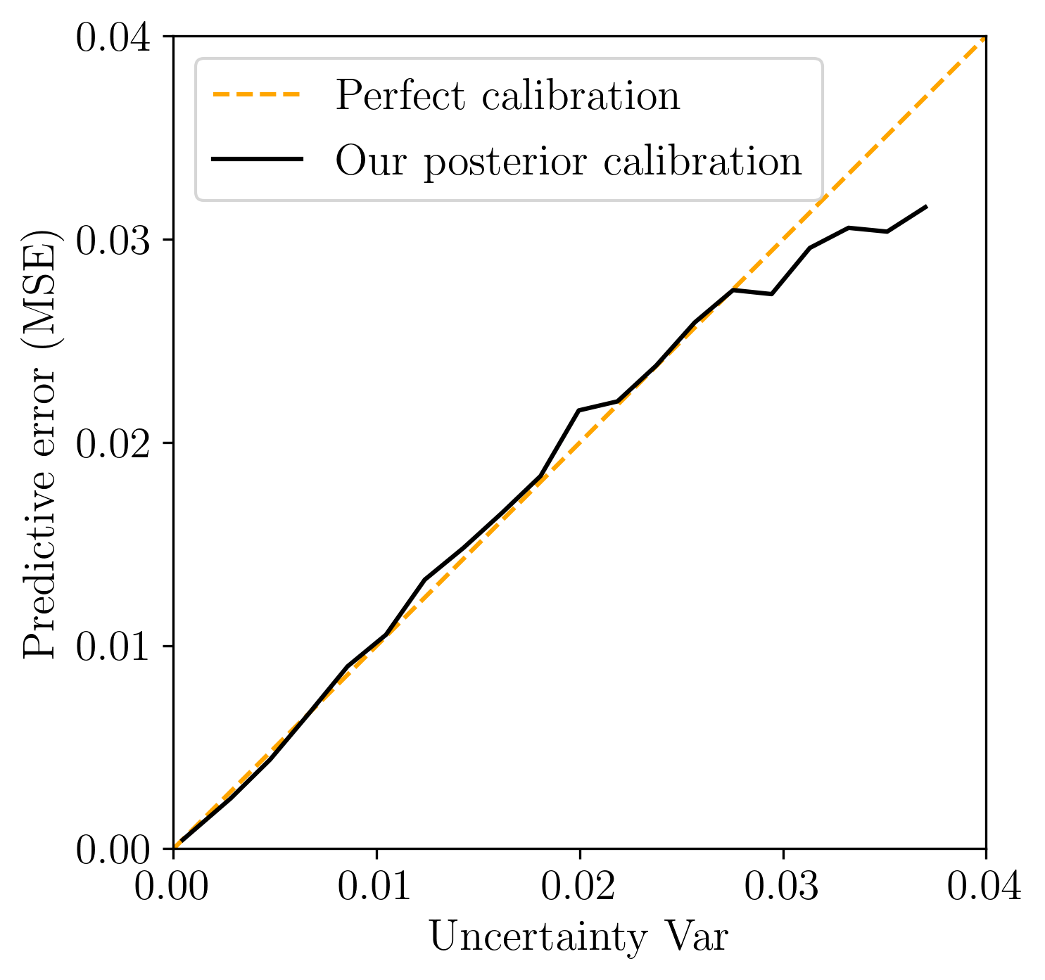
\(\textit{(ii) posterior calibration}\) by checking whether our UQ correlates with regions in the image with large errors. This important check of UQ is called calibration (C. Guo et al., 2017) and is established qualitatively by visually juxtaposing errors with UQ in Figure . For a more quantitative test, we plot a calibration line by using \(\sigma\)-scaling (Laves et al., 2020);

\(\textit{(iii) simulation-based calibration (SBC)}\) by testing for uniformity in the rank statistic when comparing various samples drawn from the proposed posterior with the known prior (Talts et al., 2018,Radev et al. (2020)).

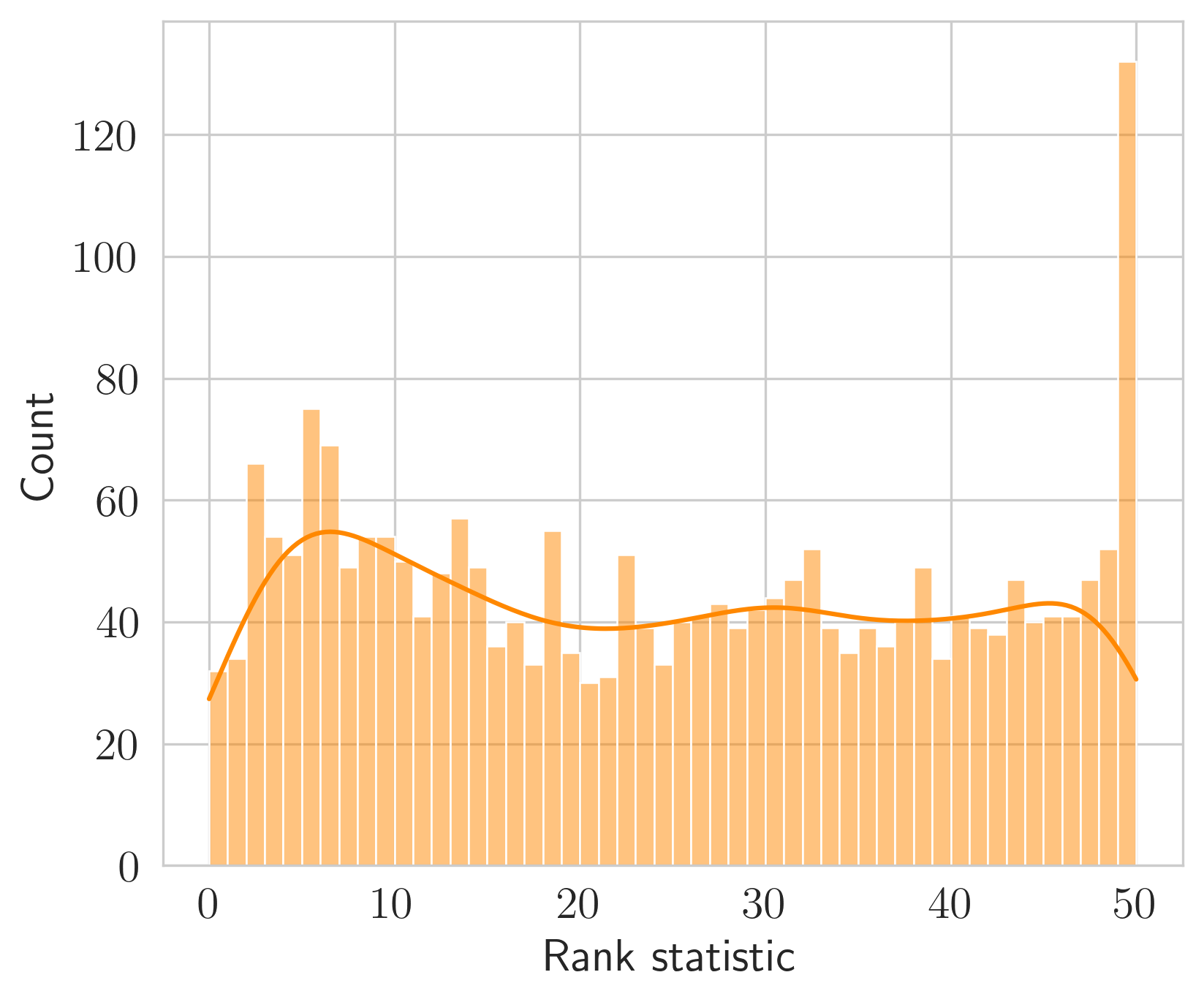
The results of these three tests are included in Figure and show our learned posterior is consistent and approximates the true posterior. For this reason, we argue that a practitioner is justified in using our posterior for uncertainty quantification.

NEW WORK TO BE PRESENTED:

We have two main contributions.

\(\textit{(i)}\) Theoretical discussion on when adjoint preprocessing gives an equivalent posterior.

\(\textit{(ii)}\) Demonstration of advantages of adjoint preprocessing on two realistic medical imaging applications. (CT examples are omitted due to space concerns. They will be added in manuscript).

CONCLUSIONS:

For linear operators and Gaussian noise, we prove that adjoint preprocessing posterior is equivalent to the original posterior \(p(\mathbf{x}|\mathbf{A}^{\ast}\mathbf{y}) = p(\mathbf{x}|\mathbf{y})\). Although the distributions are ultimately the same, learning them poses different computational burdens for ML training. We showed that the adjoint accelerates convergence of CNFs for AVI. We expect the same gains to be enjoyed by other ML-based methods such as GANs, VAE’s or recently developed diffusion models (Saharia et al., 2022). We also demonstrate that the adjoint allows us to train a single network to handle many different imaging configurations thus saving engineering costs associated with designing network architectures for individual configurations. Our amortized posterior gives physically meaningful uncertainties that we also validate.

References

Adler, J., and Öktem, O., 2018, Deep bayesian inversion: ArXiv Preprint ArXiv:1811.05910.
Adler, J., Lunz, S., Verdier, O., Schönlieb, C.-B., and Öktem, O., 2022, Task adapted reconstruction for inverse problems: Inverse Problems, 38, 075006.
Antun, V., Renna, F., Poon, C., Adcock, B., and Hansen, A. C., 2020, On instabilities of deep learning in image reconstruction and the potential costs of aI: Proceedings of the National Academy of Sciences, 117, 30088–30095.
Ardizzone, L., Kruse, J., Wirkert, S., Rahner, D., Pellegrini, E. W., Klessen, R. S., … Köthe, U., 2018, Analyzing inverse problems with invertible neural networks: ArXiv Preprint ArXiv:1808.04730.
Banerjee, A., Guo, X., and Wang, H., 2005, On the optimality of conditional expectation as a bregman predictor: IEEE Transactions on Information Theory, 51, 2664–2669.
Baptista, R., Cao, L., Chen, J., Ghattas, O., Li, F., Marzouk, Y. M., and Oden, J. T., 2022, Bayesian model calibration for block copolymer self-assembly: Likelihood-free inference and expected information gain computation via measure transport: ArXiv Preprint ArXiv:2206.11343.
Bauer, S., Seitel, A., Hofmann, H., Blum, T., Wasza, J., Balda, M., … Maier-Hein, L., 2013, Real-time range imaging in health care: A survey: In Time-of-flight and depth imaging. sensors, algorithms, and applications (pp. 228–254). Springer.
Bhadra, S., Kelkar, V. A., Brooks, F. J., and Anastasio, M. A., 2021, On hallucinations in tomographic image reconstruction: IEEE Transactions on Medical Imaging, 40, 3249–3260.
Blei, D. M., Kucukelbir, A., and McAuliffe, J. D., 2017, Variational inference: A review for statisticians: Journal of the American Statistical Association, 112, 859–877.
Deans, M. C., 2002, Maximally informative statistics for localization and mapping: In Proceedings 2002 iEEE international conference on robotics and automation (cat. no. 02CH37292) (Vol. 2, pp. 1824–1829). IEEE.
Dima, A., and Ntziachristos, V., 2012, Non-invasive carotid imaging using optoacoustic tomography: Optics Express, 20, 25044–25057.
Dinh, L., Sohl-Dickstein, J., and Bengio, S., 2016, Density estimation using real nvp: ArXiv Preprint ArXiv:1605.08803.
Gelman, A., Carlin, J. B., Stern, H. S., and Rubin, D. B., 1995, Bayesian data analysis: Chapman; Hall/CRC.
Gershman, S., and Goodman, N., 2014, Amortized inference in probabilistic reasoning: In Proceedings of the annual meeting of the cognitive science society (Vol. 36).
Ghosal, S., and Van der Vaart, A., 2017, Fundamentals of nonparametric bayesian inference: (Vol. 44). Cambridge University Press.
Gravel, P., Beaudoin, G., and De Guise, J. A., 2004, A method for modeling noise in medical images: IEEE Transactions on Medical Imaging, 23, 1221–1232.
Guo, C., Pleiss, G., Sun, Y., and Weinberger, K. Q., 2017, On calibration of modern neural networks: In International conference on machine learning (pp. 1321–1330). PMLR.
Hadamard, J., 1902, Sur les problèmes aux dérivées partielles et leur signification physique: Princeton University Bulletin, 49–52.
Kingma, D. P., and Dhariwal, P., 2018, Glow: Generative flow with invertible 1x1 convolutions: Advances in Neural Information Processing Systems, 31.
Kovachki, N., Baptista, R., Hosseini, B., and Marzouk, Y., 2020, Conditional sampling with monotone gANs: ArXiv Preprint ArXiv:2006.06755.
Kruse, J., Detommaso, G., Scheichl, R., and Köthe, U., 2019, HINT: Hierarchical invertible neural transport for density estimation and bayesian inference: ArXiv Preprint ArXiv:1905.10687.
Laves, M.-H., Ihler, S., Fast, J. F., Kahrs, L. A., and Ortmaier, T., 2020, Well-calibrated regression uncertainty in medical imaging with deep learning: In Medical imaging with deep learning (pp. 393–412). PMLR.
Oja, H., 1999, Affine invariant multivariate sign and rank tests and corresponding estimates: A review: Scandinavian Journal of Statistics, 26, 319–343.
Ongie, G., Jalal, A., Metzler, C. A., Baraniuk, R. G., Dimakis, A. G., and Willett, R., 2020, Deep learning techniques for inverse problems in imaging: IEEE Journal on Selected Areas in Information Theory, 1, 39–56.
Orozco, R., Siahkoohi, A., Rizzuti, G., Leeuwen, T. van, and Herrmann, F. J., 2021, Photoacoustic imaging with conditional priors from normalizing flows: In NeurIPS 2021 workshop on deep learning and inverse problems.
Pearl, J., 1988, Probabilistic reasoning in intelligent systems: Networks of plausible inference: Morgan kaufmann.
Penrose, R., 1955, A generalized inverse for matrices: In Mathematical proceedings of the cambridge philosophical society (Vol. 51, pp. 406–413). Cambridge University Press.
Radev, S. T., Mertens, U. K., Voss, A., Ardizzone, L., and Köthe, U., 2020, BayesFlow: Learning complex stochastic models with invertible neural networks: IEEE Transactions on Neural Networks and Learning Systems.
Rizzuti, G., Siahkoohi, A., Witte, P. A., and Herrmann, F. J., 2020, Parameterizing uncertainty by deep invertible networks: An application to reservoir characterization: In Seg technical program expanded abstracts 2020 (pp. 1541–1545). Society of Exploration Geophysicists.
Robert, C. P., Casella, G., and Casella, G., 1999, Monte carlo statistical methods: (Vol. 2). Springer.
Saharia, C., Chan, W., Saxena, S., Li, L., Whang, J., Denton, E., … others, 2022, Photorealistic text-to-image diffusion models with deep language understanding: ArXiv Preprint ArXiv:2205.11487.
Schwab, J., Antholzer, S., Nuster, R., and Haltmeier, M., 2018, Real-time photoacoustic projection imaging using deep learning: ArXiv Preprint ArXiv:1801.06693.
Siahkoohi, A., Orozco, R., Rizzuti, G., and Herrmann, F. J., 2022a, Wave-equation-based inversion with amortized variational bayesian inference: ArXiv Preprint ArXiv:2203.15881.
Siahkoohi, A., Rizzuti, G., Orozco, R., and Herrmann, F. J., 2022b, Reliable amortized variational inference with physics-based latent distribution correction: ArXiv Preprint ArXiv:2207.11640.
Sun, H., and Bouman, K. L., 2020, Deep probabilistic imaging: Uncertainty quantification and multi-modal solution characterization for computational imaging: ArXiv Preprint ArXiv:2010.14462, 9.
Talts, S., Betancourt, M., Simpson, D., Vehtari, A., and Gelman, A., 2018, Validating bayesian inference algorithms with simulation-based calibration: ArXiv Preprint ArXiv:1804.06788.
Tarantola, A., 2005, Inverse problem theory and methods for model parameter estimation: SIAM.
Whang, J., Lindgren, E., and Dimakis, A., 2021, Composing normalizing flows for inverse problems: In International conference on machine learning (pp. 11158–11169). PMLR.
Zhang, Y., Wang, Y., and Zhang, C., 2012, Total variation based gradient descent algorithm for sparse-view photoacoustic image reconstruction: Ultrasonics, 52, 1046–1055.
Zhao, X., Curtis, A., and Zhang, X., 2022, Bayesian seismic tomography using normalizing flows: Geophysical Journal International, 228, 213–239.