Accelerating innovation with software abstractions for scalable computational geophysics

Summary

We present the SLIM open-source software framework for computational geophysics, and more generally, inverse problems based on the wave-equation (e.g., medical ultrasound). We developed a software environment aimed at scalable research and development by designing multiple layers of abstractions. This environment allows the researchers to easily formulate their problem in an abstract fashion, while still being able to exploit the latest developments in high-performance computing. We illustrate and demonstrate the benefits of our software design on many geophysical applications, including seismic inversion and physics-informed machine learning for geophysics(e.g., loop unrolled imaging, uncertainty quantification), all while facilitating the integration of external software.

Introduction

Software development for exploration geophysics has been traditionally driven by performance. Though this has resulted in very efficient code, the usability and portability of these codes has been compromised as a result of the absence of user-level design. Abstractions and user interfaces at a high level have been developed in recent decades to facilitate research and development. A number of such interfaces are available, ranging from programming languages, e.g., Python (Rossum and Drake, 2009), Julia (???), and Matlab, to domain-specific languages (DSLs), including RVL (Padula et al., 2009), Firedrake (Rathgeber et al., 2016), and Devito (M. Louboutin et al., 2019; Luporini et al., 2020). Additionally, there has been a community initiative towards open-source codes and reproducibility, led by Madagascar (Madagascar, 2017). These efforts have brought attention to the need for user abstraction to easily translate mathematics into code without having to manually refactor thousands of lines of code.

Motivated by this background, we introduce our fully open-source software SLIM framework based on high-level abstractions and separation of concerns. Our software design relies on three principles: (1) A high-level abstraction that represents the mathematical problem at hand; (2) Scalability with vertical integration of high-performance software and DSLs; (3) Inter-operability through the adoption of language standards (object oriented, multiple dispatch, inheritence, …). In the following, we will detail these three points, highlighting their importance and implementation. We will follow with some illustrations of the integration with external software to demonstrate how research and development can be eased and potentially accelerated by these design principles.

Software design

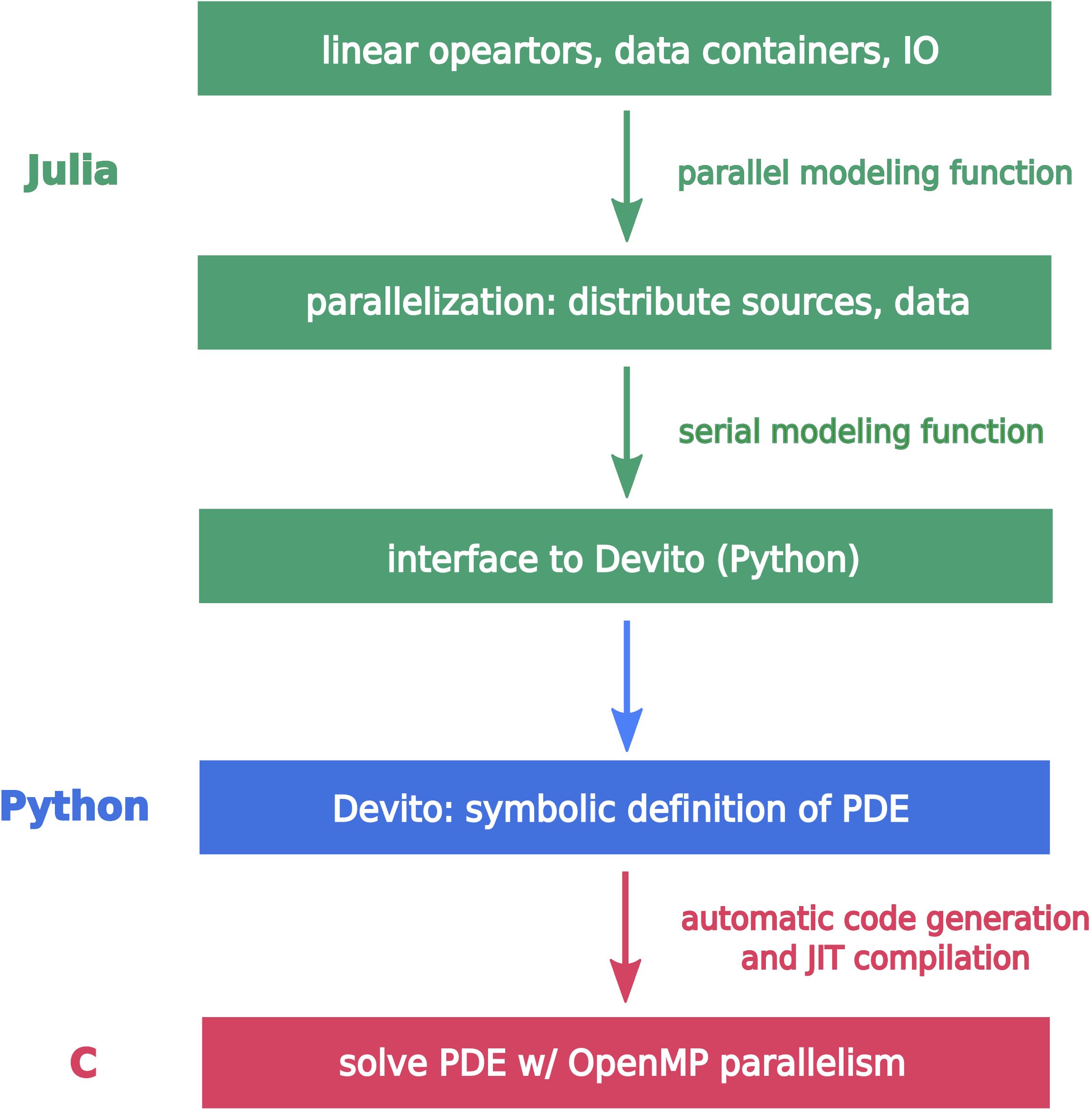
The fundamental objective of a scientific software framework is to provide users with an interface that allows them to express their own scientific problems. In particular, the interface should provide abstractions to define the problem as closely as possible to its mathematical formulation. With this design philosophy, research and development turnaround time can be drastically reduced with quick prototyping and testing of new ideas and algorithms. Our software framework is grounded in this idea and led to the development of legacy software (Lin and Herrmann, 2015; Silva and Herrmann, 2019) adopted by industry for real-world application. Based on these ideas and modern programming paradigms, we designed a high-level framework that encapsulates the mathematical definition of geoscientific problems at every level. These different levels are handled through the vertical integration of domain-specific languages (DSLs). At the lowest level, Devito provides a symbolic DSL for the definition of wave-equation and a just-in-time compiler to target the available hardware with near-optimal performance. On top of Devito, we developed JUDI, a linear algebra DSL for wave-equation based modeling and inversion. Finally, we created a machine learning framework that allows us to integrate Devito propagators and JUDI Linear Operators into machine learning (ML) frameworks (PyTorch and Flux) opening the door to ML-augmented geophysical inverse problems and uncertainty quantification (UQ). Finally, throughout these different layers, we committed to follow language standards allowing easy interfacing and integration with external software and frameworks.

Wave-equation based inversion

Linear operators are at the core of applied geophysics. Some relevant examples include data filtering tools such as Fourier-based f-k filters, the Radon transform, NMO corrections to traditional imaging operator such as Kirchhoff migration, post-stack migration and wave-equation based inversion where the discrete wave-equation is a linear operator. One of the first frameworks for abstract matrix-free linear algebra was sPOT(Berg and Friedlander, 2009), later extended to wave-equation based inversion and distributed computing for wavefield reconstruction (Kumar, 2010). While its adoption was limited by its implementation in Matlab, such user oriented abstraction laid the ground for modern abstracted frameworks such as JOLI(Modzelewski et al., 2022) in Julia and pyLops in Python (Ravasi and Vasconcelos, 2020).

Similarly, wave-equation based inversion can be trivially formulated as simple least-squares optimization problem for the non-linear wave-equation represented as an abstract matrix \(\mathbf{A}(\mathbf{m})\) parametrized by the model parameter \(\mathbf{m}\): \[ \begin{equation*} \begin{split} \underset{\mathbf{m}}{\operatorname{minimize}} \hspace{0.2cm} \Phi(\mathbf{m}) = \sum_{i=1}^{n_s} ||\mathbf{P}_r \mathbf{A}(\mathbf{m})^{-1}\mathbf{P}_s^{\top} \mathbf{q}_i - \mathbf{d}_i ||^2_2, \\ \end{split} \end{equation*} \] Building on modern software solutions JUDI (P. A. Witte et al., 2019a; Louboutin et al., 2022a) provides a high-level interface allowing to define a solver for this problem with a few lines of code. For example, FWI using Gauss-Newton updates at each iteration can be summarized in as little as five lines (Listing 1).

# Gauss-Newton method
F = judiModeling(model, srcGeom, recGeom)
J = judiJacobain(F, q)
for j=1:maxiter
    d_pred = F*q
    fhistory_GN[j] = .5f0*norm(d_pred - d_obs)^2
    # Gauss-Newton update
    p = lsqr(J, d_pred - d_obs)
    model0.m .= proj(model0.m .- reshape(p, model0.n))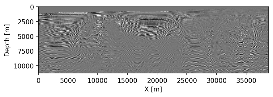
end

In addition to offering a high-level, mathematical interface to the wave-equation and related linear operators, JUDI builds on multiple layers of abstractions while still providing computational performance that is comparable to the state-of-the-art(Luporini et al., 2020). JUDI integrates Devito as a backend for the actual wave-equation solves. Devito is a stencil DSL (M. Louboutin et al., 2019; Luporini et al., 2020) that offers a symbolic user-level interface to the underlying numerical solver. This symbolic interface allows the user to easily and mathematically define generic partial differential equations (PDEs), such as the acoustic, tilted-transverse-isotropic (TTI), or elastic wave-equations. The underlying software then provides a code generation framework than can generate highly-performant code for numerous architectures, (CPU, GPUs, ARM, POWER). Its ease of use and high-level interface have contributed to its adoption in the oil-and-gas industry for production and research at scale (Washbourne et al., 2021). We summarize the vertical integration of the different technologies (compiler, Devito, JUDI, …) in Figure 1, which highlights the different levels of abstraction. The 2007 BP TTI dataset, for example, can be setup and processed with RTM within days. The results are shown in Figure 2.

Interoperability

While a proper separation of concerns can lead to highly usable, portable, and performant software, another important aspect to consider is interoperability, namely the ability to integrate software from different sources and organizations. We now describe how the design of our software framework allows for easy interfacing with external frameworks. One major drawback of proprietary and low-level software is the limited capability to interface and interact with external software. Through open-source code development, and committing to language-specific standards (such as proper usage of types, hierarchy, inheritance, etc.) in Julia and Python, we enable seamless interoperability with external software and frameworks. This greatly increases the ability to perform research, which involves being able to easily test and combine different ideas. For instance, we combine core Julia packages, our numerical optimization toolbox SlimOptim.jl (Louboutin and Herrmann, 2021a), a constrained optimization software SetIntersectionProjection.jl (Peters and Herrmann, 2019), and COFII’s wave-equation propagators (Washbourne et al., 2021), in order to setup a full waveform inversion (FWI) exercise. We were able to perform FWI, in parallel, on the Marmousi-II model by taking advantage of the best technology available. Additionally, this demonstrative example, and in general JUDI (or COFII), can trivially be deployed in the cloud using once again dedicated software abstractions (Washbourne et al., 2021; Louboutin et al., 2022b).

function objective(F, velocity, d_obs)
    J = jacobian(F, velocity)
    d_pred = F * velocity # Forward modeling with COFFI
    G = J' * ({d_pred.- d_obs) # Gradient with COFII
    f = .5f0*norm(d_pred .- d_obs)^2 # Misfit
    return f, G
end
# Projection on TV+bounds, SetIntersectionProjection.jl
prj = setup_projection(...)
# Projected Quasi-Newton (l-BFGS) with SlimOptim.jl
sol = pqn(x->objective(F, x, d_obs), vec(v2), prj);

Since different software modules can be pieced together with minimal effort, it greatly aids the development and testing of new research. This flexibility allows, for instance, the integration of machine learning into conventional algorithm pipelines in a plug-and-play fashion. In the following section, we provide some notable examples of this approach.

Machine learning

Thanks to recent theoretical and practical advances, deep learning has seen a wide adoption in various geophysical applications ranging from processing (e.g., denoising, multiple removal) to inverse problems and seismic interpretation (e.g., G. Zhang et al., 2018; B. Wang et al., 2019; Yang and Ma, 2019). One of the core challenges in the adoption of deep learning for seismic applications is the integration of existing codes (e.g. seismic propagators) into deep-learning frameworks based on automatic differentiation (AD). To be able to differentiate through networks that contain both standard PyTorch/Tensorflow layers, as well as third party functions, such as a forward modeling kernel, the third party code must have manually implemented gradients and must be properly integrated into the deep learning framework. Our high-level linear algebra abstraction framework, which sits on top of our Devito-based propagators, facilitates this integration, as deep learning frameworks like PyTorch or Flux are already able to backpropagate through a linear operator (namely by applying its adjoint to the data residual). This allows us to implement deep neural networks in Flux, in which we can combine standard deep learning layers with external third party functions, e.g. convolutional layers with migration/demigration operators. This capability has enabled various research projects in our group, including surface-related multiple elimination (Siahkoohi et al., 2019c), dispersion attenuation (Siahkoohi et al., 2019b), and ML-augmented imaging and uncertainty quantification (Siahkoohi et al., 2019a, 2020). We show in the following two examples of machine learning for exploration geophysics that take advantage of these high-level abstractions to interface PDE solvers (JUDI, Devito) with deep learning frameworks.

Seismic imaging with deep priors and uncertainty quantification

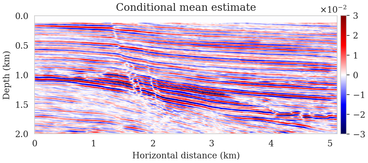
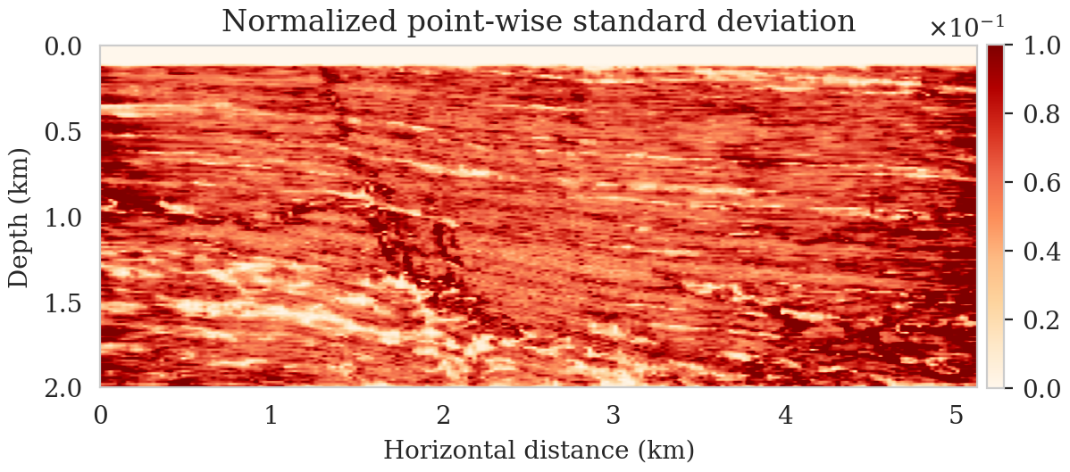
Since we can integrate Devito’s highly optimized wave-equation solvers with the PyTorch deep learning library, we propose to use deep priors (Lempitsky et al., 2018) to regularize seismic imaging, where we reparameterize the seismic image as the output of an untrained convolutional neural network (CNN). This approach acts as a regularization in the image space (Lempitsky et al., 2018; Cheng et al., 2019; Dittmer et al., 2020), which exploits the inductive bias of the CNN in representing images without noisy artifacts (Lempitsky et al., 2018). We perform Bayesian inference via a gradient-based Markov chain Monte Carlo (MCMC) algorithm (Welling and Teh, 2011), where each iteration requires differentiating the action of the linearized Born scattering operator on the CNN output with respect to the CNN’s weights. In order to have access to the automatic differentiation utilities of PyTorch, we expose Devito’s matrix-free implementations for the migration operator and its adjoint to PyTorch via Devito4PyTorch (Siahkoohi and Louboutin, 2021). This is exemplified in Listing 3. Figure 3 summarizes the results of seismic imaging and uncertainty quantification with this approach, which are borrowed from Siahkoohi et al. (2021).

def deep_prior_imaging(d_obs, n, maxiter=1000):
    # PyTorch Integrated Devito Jacobian.
    J = ForwardBornLayer(model, geometry)
    # Initialize deep prior CNN with random input.
    G = deep_prior_net()
    z = torch.randn([1, 1, n[1], n[2]])
    # Setup pSGLD MCMC sampler.
    optim, samples = pSGLD(G.parameters(), lr=0.001), []
    for i in range(maxitr):
        # Compute predicted perturbation model and data.
        x = G(z)
        d_pred = J(x)
        # Compute the negative log-posterior.
        nlp = n_log_posterior(d_pred, d_obs, G.parameters())
        # Compute the gradient w.r.t. the CNN weights,
        nlp.backward()
        # Sample with pSGLD.
        optim.step()
        samples.append(x.detach().numpy())
    return samples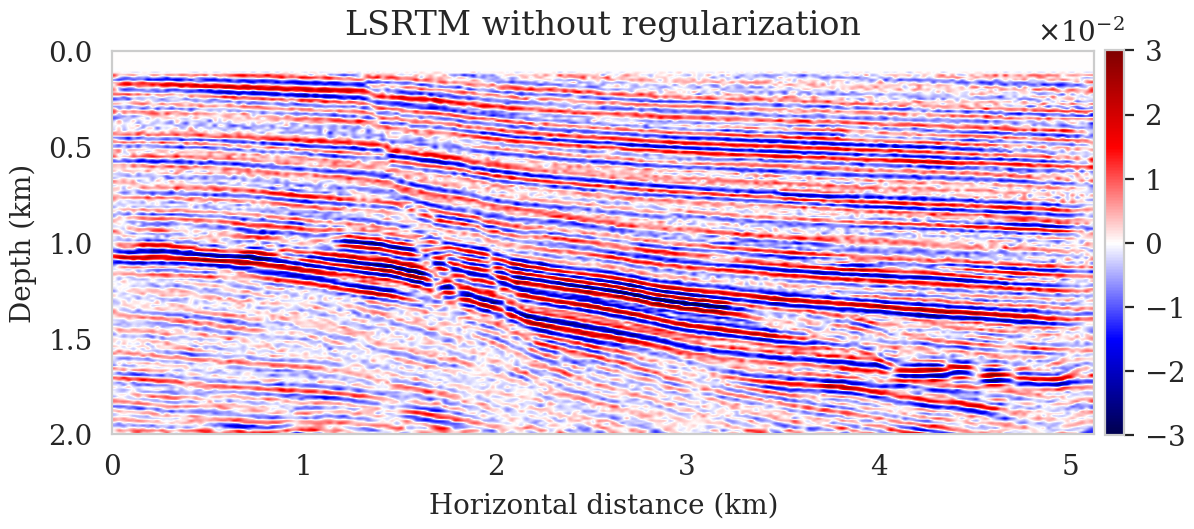

Loop-unrolled seismic imaging

Another set of applications that are enabled by the proper integration of abstract seismic modeling operators into deep learning frameworks are loop-unrolled optimization algorithms such as the learned primal-dual reconstruction (Andrychowicz et al., 2016; Adler and Öktem, 2018). These are special types of networks that follows the general structure of gradient-based optimization algorithms, in which conventional gradients are augmented by additional neural network layers. Using our integration of JUDI operators into Flux via the JUDI4Flux package (P. A. Witte et al., 2019b), we apply the loop-unrolled network architecture from (Adler and Öktem, 2017) to seismic imaging. Every iteration of the loop-unrolled algorithm consists of computing the (conventional) gradient of the LS-RTM objective function \(g\), using the forward and adjoint linearized Born scattering operator, followed by the application of a shallow CNN (Listing 4). The network takes a single simultaneous (super-) shot record as the input and predicts an LS-RTM (or true) image. We train the network in a supervised fashion, in which we minimize the misfit between the predicted image and the true image (whereas in reality, one would train with available LS-RTM images). Figure 4 shows the output of the loop-unrolled gradient descent algorithm, Listing 4, after training the network for 2000 iterations on a training dataset of 2,000 data-image pairs. The example is not meant to represent a realistic scenario (as the true images which were used in the training process are obviously unknown), but serve as a proof of concept on how to augment physical models with data-driven approaches. The complete example and additional variations are available at LoopUnrolledSeismicImaging.

function loop_unrolled_lsrtm(d_obs, n; maxiter=10)
    x = randn(Float32, n[1], n[2], 1, 1)
    nx, ny, nc, nb = size(x)
    s = randn(Float32, nx, ny, 5, nb) # memory term
    for j=1:maxiter
        g = adjoint(J)*(J*vec(x) - d_obs)
        g = reshape(Flux.normalise(g), nx, ny, 1, 1)
        u = cat(x, g, s, dims=3)
        u = bn1(conv1(u)); u = bn2(conv2(u)); u = bn3(conv3(u));
        s = relu.(u[:, :, 2:6, :])
        dx = u[:, :, 1:1, :]
        x += dx
    end
    return vec(x)
end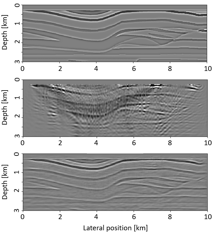

End-to-end inversion for geological carbon storage monitoring

Finally, we show that we can easily build a framework for seismic monitoring of geological carbon storage that integrates PDE solvers, deep learning models and physical constraints. These monitoring problems rely on three different types of physics (D. Li et al., 2020): fluid-flow physics, rock physics and wave physics. Given time-lapse seismic data collected over multiple years, we jointly invert for the rocks intrinsic permeability which can be used to recover the CO₂ concentration. By leveraging our high-level abstractions and AD, we can directly differentiate through all three physics solvers which map permeability to seismic data and minimize a fully coupled data misfit objective function. At each iteration, given an estimate of the permeability \(K\), we model seismic data where the subsurface velocity is translated from the solution of the fluid-flow simulation. We can then compute the standard data misfit and use automatic differentiation to compute the permeability update. Because each step is abstracted, we can easily swap each physical solver with a different one, such as replacing the fluid-flow solver by a trained Fourier Neural Operator (FNO) for computational efficiency (Z. Li et al., 2020). We show in Figure 5 that we can recover the permeability from seismic measurements using a pre-trained FNO in place of a fluid-flow solver.

opt = RMSprop()
for j=1:maxiter
    theta = params(K)
    grads = gradient(theta) do
        c = S(K); v = R(c); d_pred = F(v)
        return 0.5f0 * norm(d_pred-d_obs)^2f0
    end
    for p in theta
        update!(opt, p, grads[p])
    end
end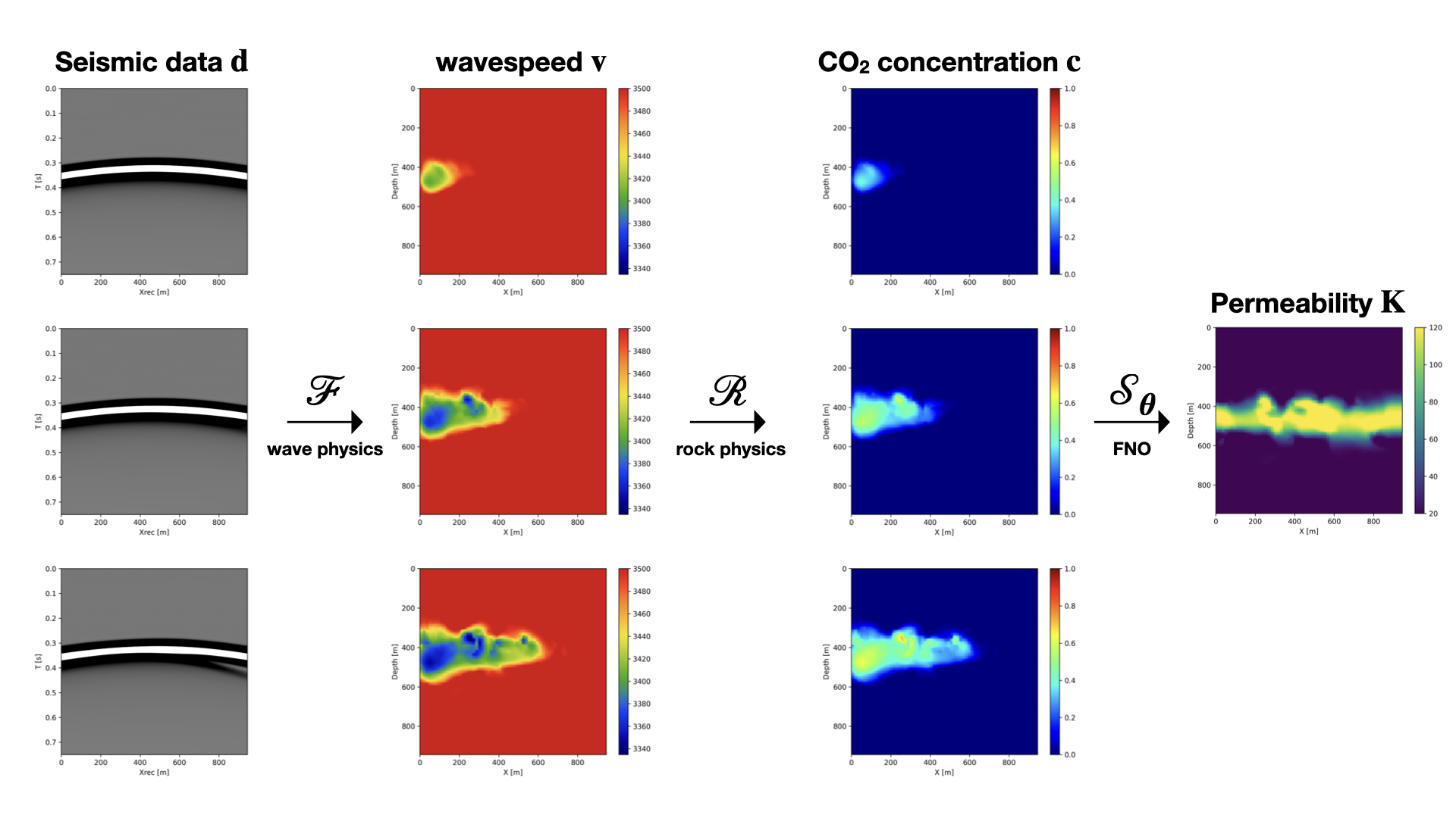

Conclusions

Through this paper, we have introduced a software design philosophy aimed at enabling research and development at scale in geoscience, with the potential to generalize to any inverse problem such as medical imaging. We demonstrated through carefully chosen example that high-level abstractions allow to express complex problem in a clear and representative way without incurring additional computational costs. Our software framework already allows for a wide range of application, including industry scale inversion and cutting-edge physics-informed deep learning for geophysics. We intend to build additional capabilities to tackle modern computing environment such as Cloud computing, task dedicated accelerators (i.e TPUs) and non-convex optimization.

Acknowledgment

This research was carried out with the support of Georgia Research Alliance and partners of the ML4Seismic Center. We thank J. Washbourne at CVX for the fruitful discussions on open source software development and interoperability.