Neural network augmented wave-equation simulation

Ali Siahkoohi, Mathias Louboutin, and Felix J. Herrmann
School of Computational Science and Engineering
Georgia Institute of Technology
{alisk, mlouboutin3, felix.herrmann}@gatech.edu

Introduction

In inverse problem, we heavily rely on having an accurate forward modeling operators. Often, we can not afford being physically or numerically accurate. In other words, being numerically inaccurate can be due to computationally complexity of accurate methods, or incomplete knowledge of the underlying data generation process. In either case, motivated by Ruthotto and Haber (2018), we propose to intersperse CNNs between timestepping algorithm for simulating acoustic wave-equation. We mimic incomplete/inaccurate physics by simulating wave equation with finite-difference method, while utilizing a poor (second-order) discretization of Laplacian.

Conventional method for solving partial differential equations (PDEs), e.g., finite-difference and finite-element method, given enough computational recourses, are able to simulate high-fidelity solutions to PDEs. On one hand, as long as the Courant–Friedrichs–Lewy conditions for stability are satisfied, finite-difference methods are able to compute solutions to PDE, regardless of medium parameters, with arbitrary precision. On the other hand, finite-element method requires careful meshing of the medium in order to carry out the simulation. Another motivation behind this work is to exploit the fact that in seismic, wave simulations are usually carried out for specific families of velocity models and source/receiver distributions. We hope our proposed method meets halfway between two mentioned extremes—i.e., being too generic (finite-difference method) and being too problem specific (finite-element method).

There are several attempts to exploit learning methods in wave-equation simulation. Raissi (2018) approximates the solution to a nonlinear PDE with a neural network. The neural network, given points on the computational grid as input, computes the solution of PDE. Training data is obtained by computing the solution of PDE on several points. Moseley et al. (2018) completely ignore the Laplacian and they solely rely on predicting the next timestep from the previous two timesteps by learning the action of the spatially varying velocity and Laplacian. While possible in principle, their approach needs to train for long times to provide reasonable simulations on relatively simple models. Siahkoohi et al. (2019) instead of ignoring the physics, relies on low-fidelity wave-equation simulation, and by exploiting transfer learning, they utilize a single CNN to correct wavefield snapshots simulated on a “nearby” velocity mode for numerical dispersion at any given timestep. In this work, we extend ideas in Siahkoohi et al. (2019) and propose using multiple CNNs, interspersed between low-fidelity timesteps. Finally, Rizzuti et al. (2019) propose interspersing Krylov-subspace iterations and neural nets while inverting the Helmholtz equation. They show improvement in convergence by “propagating” an approximated wavefield, obtained from a limited number of iterations, with the aid of a trained convolutional neural net. This technique can be seen as the frequency-domain counterpart of our proposed method.

Our paper is organized as follows. First, we describe our approach in detail by first, describing our formulation for learned wave simulation. Next, we introduce our training objective function. Due to dependencies of CNN parameters, we devised an training heuristic that we describe. Before explaining our numerical experiments, we state used CNN architecture and training details. Next, we describe our three numerical experiments we conduct and discuss effectiveness of the proposed method.

Theory

We describe how we augment low-fidelity physics with learning techniques to handle incomplete and/or inaccurate physics, where the low-fidelity physics is modeled via finite-difference method with a poor discretization of the Laplacian. To ensure accuracy, the temporal and spatial discretization in high-fidelity wave-equation simulations have to be chosen very fine, typically one to two orders of magnitude smaller than Nyquist sampling rate. As mentioned earlier, we will utilize a poor discretization (only second order) for the Laplacian to carry out low-fidelity wave-equation simulations, but the scheme can be extended to other proxies of incomplete or inaccurate physics.

Simulations by timestepping

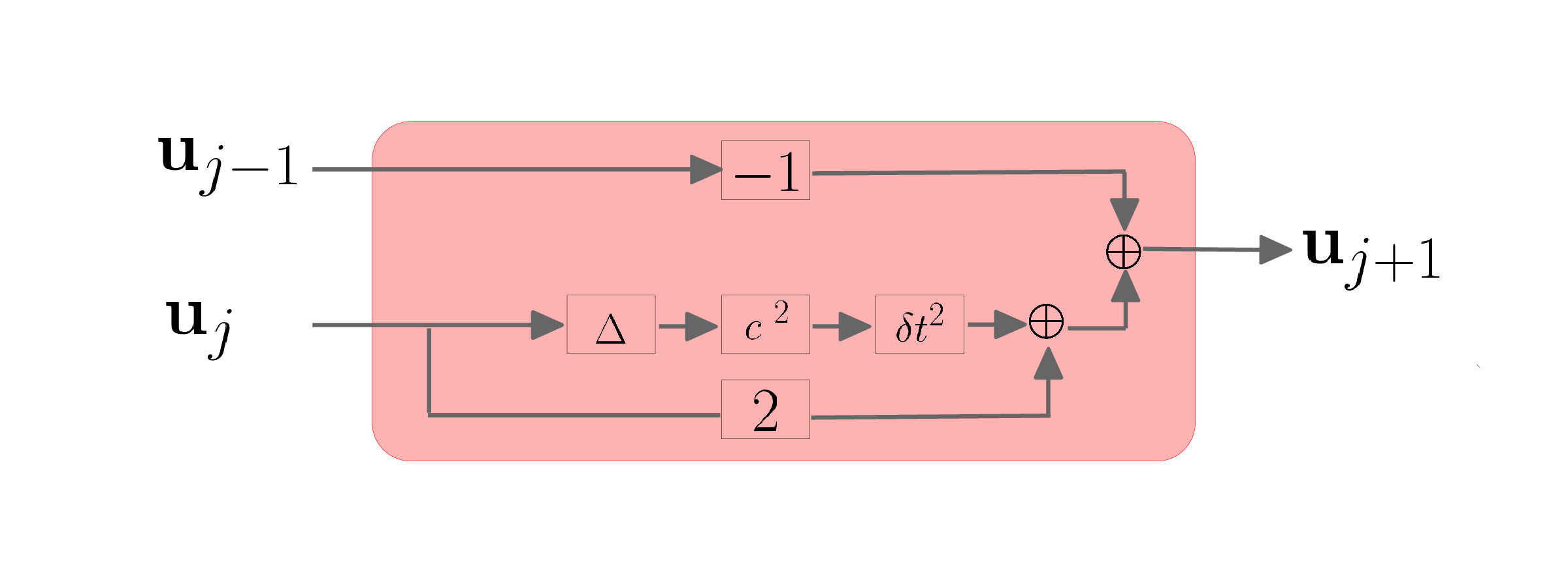
After discretization of the acoustic wave equation, a single timestep of of scalar wavefields, simulated on \(0 \leq t \leq T\), can be written as below: \[ \begin{equation} \mathbf{u}_{j+1} = 2\mathbf{u}_{j}-\mathbf{u}_{j-1}+\delta t^2\mathbf{c}^2 \mathbf{\Delta}\mathbf{u}_j, \quad j=0,1, \ldots , N-1 , \label{high-fidelity} \end{equation} \] where \(\mathbf{u}_{j}\) is the high-fidelity scalar wavefield at \(j^{\text{th}}\) timestep, \(\delta t\) is the temporal discretization (timestep), \(\mathbf{c}\) is the spatially varying velocity in the medium, and \(\mathbf{\Delta}\) is the high-order discretization of Laplacian. Similar to Equation \(\ref{high-fidelity}\), the low-fidelity timestepping equation can be formulated as \[ \begin{equation} \mathbf{\bar{u}}_{j+1} = 2\mathbf{\bar{u}}_{j}-\mathbf{\bar{u}}_{j-1}+\delta T^2\mathbf{\bar{c}}^2 \mathbf{\bar{\Delta}}\mathbf{\bar{u}}_j,\quad j=0, 1, \ldots , M-1, \label{low-fidelity} \end{equation} \] where \(\mathbf{\bar{u}}_{j}\) is the low-fidelity scalar wavefield, \(\delta T\) is the coarse timestep, \(\mathbf{\bar{c}}\) is the coarse spatially varying velocity, and \(\mathbf{\bar{\Delta}}\) is the coarse (only second second order) discretized Laplacian.

Motivated by Ruthotto and Haber (2018), we consider every timestep as a single layer in a neural network, where the discretized Laplacian is a linear operator, followed by the (nonlinear) action of the spatial varying velocity. Moreover, noticing the additional terms in the Equation \(\ref{high-fidelity}\), each timestep is similar to a residual block introduced by Szegedy et al. (2017). Figures 1a and 1b schematically indicate each timestep as a block, corresponding to high- and low-fidelity discretization of wave equation. respectively. The similarity of high- and low -fidelity timestepping method and CNNs can be perceived from Figures 2a and low-fidelity-step, respectively, where red and yellow blocks correspond to high- and low-fidelity timestepping equations, respectively.

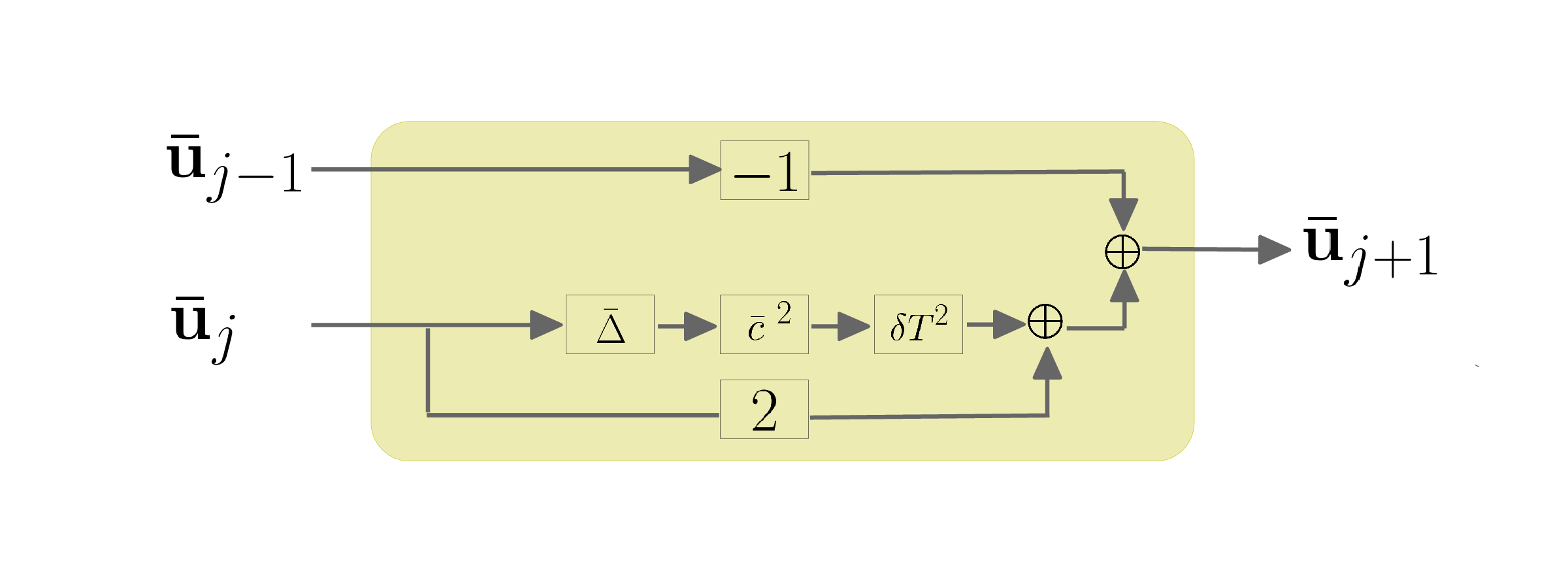
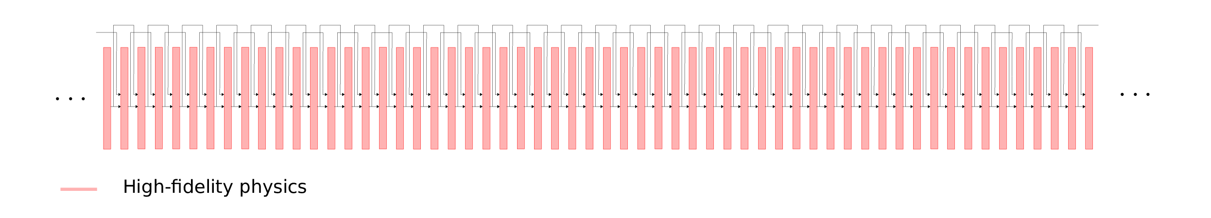
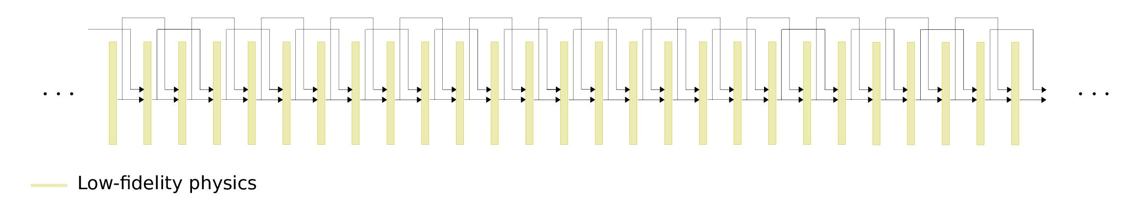
As it can be seen, high-fidelity simulation of the wave equation up to time \(t=T\) requires a lot of high-fidelity timesteps. On the other hand, Figure 2b shows that the low-fidelity simulations can be done with much less low-fidelity timesteps, due to course time sampling, which each timestep is cheaper than the high-fidelity timesteps due to the coarse discretization of Laplacian. Although computationally cheap, the low-fidelity wave-equation simulations suffer from numerical dispersion artifacts.

Learned wave simulations

Depending on the domain of application, we can assume wave simulations are typically carried out for specific families of velocity models and source/receiver distributions. This motivates us to deploy a data-driven wave simulation algorithm which is coupled with low-fidelity and cheap physics and hope to recover high-fidelity wave simulations on a family of velocity models. In our method, we propagate the coarse-grained wavefields according to Equation \(\ref{low-fidelity}\) with a coarsened Laplacian. After \(k\) timesteps, where \(k\) is a hyperparameter, we apply a correction with a CNN, \(\mathcal{G}_{\theta_i}\), parameterized by \(\theta_i\), to the obtained wavefield at \(j^{\text{th}}\) timestep and proceed with the timestepping. The proposed data-driven timestepping wave simulation method is formalized in Equation \(\ref{learned}\). \[ \begin{equation} \mathbf{\bar{u}}_{j+1} = \begin{cases} \mathcal{G}_{\theta_i}\left( 2\mathbf{\bar{u}}_{j}-\mathbf{\bar{u}}_{j-1}+\delta T^2 \mathbf{\bar{c}}^2 \mathbf{\bar{\Delta}}\mathbf{\bar{u}}_j\right), \ i = \lfloor \frac{j}{k} \rfloor & \text{ if } j\equiv k-1 \ (\bmod \ k), \\ 2\mathbf{\bar{u}}_{j}-\mathbf{\bar{u}}_{j-1}+\delta T^2 \mathbf{\bar{c}}^2 \mathbf{\bar{\Delta}}\mathbf{\bar{u}}_j & \text{ else } \end{cases} \label{learned} \end{equation} \] where \(j=0,1, \ldots , M-1\). The schematic representation of Equation \(\ref{learned}\) is illustrated in Figure 3. Yellow blocks represent low-fidelity timesteps (see Equation \(\ref{low-fidelity}\) and Figure 1b) and blue blocks correspond to CNNs, \(\mathcal{G}_{\theta_i}, \ i = 0, 1, \ldots , \lfloor \frac{M-1}{k} \rfloor\).

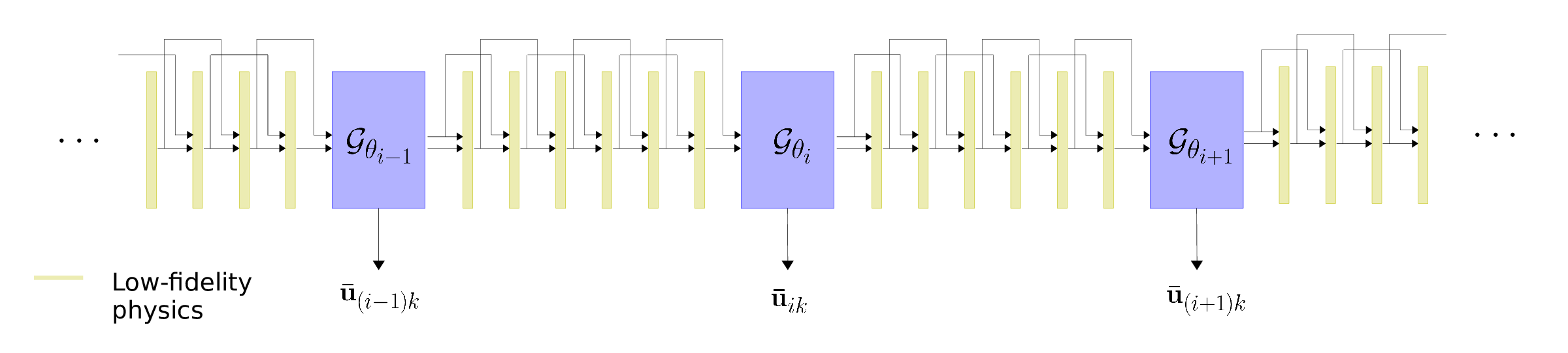
The CNNs correct for the effects of inaccurate physics—i.e., numerical dispersion in our experiments, at every \(k^{\text{th}}\) low-fidelity timestep. In this work, the parameters, \(\theta_i\), are not shared among the CNNs. We have not explored the possibility of shared weights among the CNNs in different stages of wave propagation.

Note that although parameters of the CNNs are not shared, they are not independent—i.e., after \(j^{\text{th}}\) timestep, CNN \(\mathcal{G}_{\theta_i}, i = \lfloor \frac{j}{k} \rfloor\), corrects for errors in the wavefield introduced by low-fidelity timestepping and imperfections present in the output of \((i-1)^{\text{th}}\) CNN, which have been propagated through timestepping. Therefore, a small perturbation in the parameters of a CNN in the initial stages of neural network augmented timestepping causes noticeable differences in the input of the CNNs in later stages of the wave propagation. The described dependencies among the CNN parameters introduces difficulties in optimizing the parameters of the CNNs. Below we describe our heuristic for training the CNNs.

Training objective

During training, we train all the CNNs toward the high-fidelity solution of wave-equation, at the corresponding timestep, obtained by solving Equation \(\ref{high-fidelity}\). As it can be seen from Equation \(\ref{learned}\), after \(j^{\text{th}}\) timestep, CNN \(\mathcal{G}_{\theta_i}, i = \lfloor \frac{j}{k} \rfloor\), is tasked to correct the effects of low-fidelity timestepping. During training, \(i^{\text{th}}\) CNN maps its input, \(2\mathbf{\bar{u}}_{j}-\mathbf{\bar{u}}_{j-1}+\delta T^2 \mathbf{\bar{c}}^2 \mathbf{\bar{\Delta}} \mathbf{\bar{u}}_j\), to \(\mathbf{u}_{j+1}\), result of \(j^{\text{th}}\) timestep using high-fidelity timestepping, obtained by Equation \(\ref{high-fidelity}\).

Define function \(\bar{F}_k(.)\) as the action of \(k\) low-fidelity timesteps—i.e., \(\bar{F}_k(.)\) represents \(k\) consecutive low-fidelity time stepping blocks, depicted in Figure 1b. Clearly, \(\bar{F}_k\) is only a function of \(k\), \(\delta T\), \(\mathbf{\bar{c}}\), and \(\mathbf{\bar{\Delta}}\). Using the defined notation, we can write the input to \(i^{\text{th}}\) CNN, \(\mathbf{\hat{u}}_i, \ i =0, 1, \ldots , \lfloor \frac{M-1}{k} \rfloor\), as follows: \[ \begin{equation} \begin{aligned} &\ \mathbf{\hat{u}}_i = \bar{F}_k (\mathcal{G}_{\theta_{i-1}}(\mathbf{\hat{u}}_{i-1} )), \quad i = 1, 2, \ldots , \lfloor \frac{M-1}{k} \rfloor, \\ &\ \mathbf{\hat{u}}_0 = \bar{F}_k(\mathbf{q}), \\ \end{aligned} \label{inputtoCNN} \end{equation} \] where \(\mathbf{q}\) is the source. Also let \(\mathbf{u}_{\tau_i}\) denote the wavefield obtained at \(j^{\text{th}}\) timestep of high-fidelity timestepping (Equation \(\ref{high-fidelity}\)), where \(\tau_i = j = (k+1)i-1\).

The input-output pair of the \(i^{\text{th}}\) CNN is \((\mathbf{\hat{u}}_i, \mathbf{u}_{\tau_i})\). We can generated multiple training pairs for CNNs by simulating \((\mathbf{\hat{u}}_i, \mathbf{u}_{\tau_i})\) pairs, for various velocity models and source locations. Assume we have \(n\) pairs of of training data for CNNs, namely, \((\mathbf{\hat{u}}_i^{(p)}, \mathbf{u}_{\tau_i}^{(p)}), \ p = 0,1, \ldots , n-1\). The objective function for optimizing \(i^{\text{th}}\) CNN can be written as follows: \[ \begin{equation} \begin{split} \mathcal{L}_i = \frac{1}{n} \sum_{p=0}^{n-1} \left \| \mathcal{G}_{\theta_i}(\mathbf{\hat{u}}_i^{(p)}) - \mathbf{u}_{\tau_i}^{(p)} \right \|_1, \quad i = 0, 1, \ldots , \lfloor \frac{M-1}{k} \rfloor . \\ \end{split} \label{trainCNN-i} \end{equation} \] In the past, in a similar attempt, we used Generative Adversarial Networks (GANs, Goodfellow et al., 2014) to train a CNN in order to remove numerical dispersion from wavefield snapshots (Siahkoohi et al., 2018, 2019). In this work we choose to use \(\ell_1\) norm as the misfit function based on two reasons. First, training GANs is computationally expensive since it requires training an additional neural network that discerns between high-fidelity wavefield snapshots and corrected ones. The computational complexity of the proposed method in this work is significantly higher than our previous attempts (Siahkoohi et al., 2018, 2019), because it involves training multiple CNNs. Based on the mentioned facts, for limiting the computation time we chose to use \(\ell_1\) misfit function. Second, motivated by a numerical experiment performed by Hu et al. (2019), \(\ell_1\) norm misfit function yields the second best results after the misfit function utilizing a combination of GANs and \(\ell_1\) norm misfit. In the next section, we describe our heuristic for training the CNNs.

Training heuristic

To overcome complexities caused by dependencies between parameters of CNNs, we optimize the objective functions \(\mathcal{L}_i\) with a heuristic described below. We minimize \(\mathcal{L}_i, \ i = 0, 1, \ldots , \lfloor \frac{M-1}{k} \rfloor\), with respect to \(\theta_i\), respectively. In other words, we minimize \(\mathcal{L}_i\) with respect to \(\theta_i\), by keeping the rest of the parameters fixed. We keep updating all the set of parameters, in a cyclic fashion—i.e., once we updated all the parameters, \(\mathcal{L}_i, \ i = 0, 1, \ldots , \lfloor \frac{M-1}{k} \rfloor\), we start over and update them again, in order, until a stopping criteria is achieved. We will describe the stopping criteria used in our experiments later.

We minimize objective functions the above objectives \(\ref{trainCNN-i}\) with a variant of Stochastic Gradient Descent known as the Adam optimizer (Kingma and Ba, 2015) with momentum parameter \(\beta = 0.9\) and a linearly decaying stepsize with initial value \(\mu = 2 \times 10^{-4}\) for both the generator and discriminator networks. During each iteration of Adam, the gradient \(\mathcal{L}_i\) is approximated by a single randomly selected training pair. These pairs are selected without replacement. Once all the training pairs have been selected, we start over by randomly picking training pairs, without replacement from the entire training set.

The optimization carries out for a predetermined number of total iterations, where each iterations consists of drawing a random training pair, without replacement, and updating parameters of a CNN. Additionally, while optimizing \(\theta_i\) by keeping the rest of the parameters fixed, before proceeding to the next set of parameters, we carry out the optimization to update \(\theta_i\) for number of iterations, which we refer to it as mini-iterations. Algorithm 1 indicates the steps for optimizing objective functions \(\ref{trainCNN-i}\).

  1. INPUT: 
      \(MaxItr \quad\)  // total number of iterations to carry out the optimization
      \(MaxMiniItr \quad\)  // mini-iterations before proceeding to the next CNN
      \(\bar{F}_k(.) \quad\) // k consecutive low-fidelity time stepping blocks
      \(\mathbf{q}^{(p)} \ p = 0,1, \ldots , n-1 \quad\) \\ sources corresponding to different training pairs
      \(\mathbf{u}_{\tau_i}^{(p)}, \ p = 0,1, \ldots , n-1, \ i = 0, 1, \ldots , \lfloor \frac{M-1}{k} \rfloor \quad\) \\ high-fidelity snapshots
      \({\theta^0_i}, \ i = 0, 1, \ldots , \lfloor \frac{M-1}{k} \rfloor \quad\) // randomly initialized parameters
  2. \(ItrNum \leftarrow 0\)
  3. FOR \(i = 0:\lfloor \frac{M-1}{k} \rfloor\) DO
  4.      \(\theta_i = \theta^0_i\)
  5. FOR \(p = 0:n-1\) DO
  6.      \(\mathbf{\hat{u}}_0^{(p)} = \bar{F}_k(\mathbf{q}^{(p)})\)
  7. WHILE \(itrNum < MaxItr\) DO
  8.      FOR \(i = 0:\lfloor \frac{M-1}{k} \rfloor\) DO
  9.          IF \(i>0\) DO
  10.             FOR \(p = 0:n-1\) DO
  11.                 \(\mathbf{\hat{u}}_i^{(p)} = \bar{F}_k(\mathcal{G}_{\theta_{i-1}}(\mathbf{\hat{u}}_{i-1}^{(p)}))\)
  12.         FOR \(miniItrNum = 1:MaxMiniItr\) DO
  13.             \(p \leftarrow SampleWithoutReplacement(\left \{ 0,1, \ldots , n-1 \right \})\)
  14.             \(\theta_i \leftarrow \mathop{\arg \min}_{\theta_i} \left \| \mathcal{G}_{\theta_i}(\mathbf{\hat{u}}_i^{(p)}) - \mathbf{u}_{\tau_i}^{(p)} \right \|_1\)
  15.             \(ItrNum \leftarrow ItrNum + 1\)
  16. RETURN \({\theta_i}, \ i = 0, 1, \ldots , \lfloor \frac{M-1}{k} \rfloor\)

CNN architecture

Motivated by our previous attempts for numerical dispersion removal from wavefield snapshots (Siahkoohi et al., 2018, 2019), we use the exact architecture provided by Johnson et al. (2016), which includes Residual Blocks, the main building block of ResNets, introduced by He et al. (2016), for all the CNNs \(\mathcal{G}_{\theta_i}, \ i = 0, 1, \ldots , \lfloor \frac{M-1}{k} \rfloor\).

Training details and implementation

While CNNs are known to generalize well—i.e., maintain the quality of performance when applied to unseen data, they can only be successfully applied to a data set drawn from the same distribution as the training data. Because of the Earth’s heterogeneity and complex geological structures present in realistic-looking models, training a neural network that can generalize well when applied to another velocity model can become challenging. While we have successfully demonstrated that transfer learning (Yosinski et al., 2014) can be used in situations where the neural network is initially trained on data from a proximal survey (Siahkoohi et al., 2019), we chose in this contribution, as a proof of concept, to keep the velocity model fixed, and vary the source locations to generate different training/testing pairs.

We use the Marmousi velocity model and out of \(401\) available shot locations with \(7.5\) \(\mathrm{m}\) spacing, we allocate half of the shot locations to training and use the rest of the shot locations to generate testing pairs, for evaluation purposes. The maximum simulation time in our experiments in \(1.1\) \(\mathrm{s}\).

We designed and implemented our deep architectures in TensorFlow¹. To carry out our wave-equation simulations with finite differences, we used Devito² (Louboutin et al., 2018; Luporini et al., 2018). We used the functionality of Operator Discretization Library³ to wrap Devito operators into a TensorFlow layers. Our implementation can be found on GitHub⁴.

We ran our algorithm on Amazon Web Services’ g3.4xlarge instance, where we optimize the CNN parameters on a NVIDIA Tesla M60 GPU and Devito utilizes \(16\) CPU cores to perform finite-difference wave-equation simulations. Initially, we simulate the high-fidelity training wavefield snapshots, \(\mathbf{u}_{\tau_i}^{(p)}, \ p = 0,1, \ldots , n-1, \ i = 0, 1, \ldots , \lfloor \frac{M-1}{k} \rfloor\), only once, in the beginning, and store them. In order to limit CPU-GPU communication, before utilizing the GPU to to update \({\theta_i}, \ i = 0, 1, \ldots , \lfloor \frac{M-1}{k} \rfloor\), we generate the input to \(i^{\text{th}}\) CNN, \(\mathbf{\hat{u}}_i^{(p)}, \ p = 0,1, \ldots , n-1\) all at once, and store them. Afterwards, \(i^{\text{th}}\) CNN can be (re)trained using the stored input/output wavefield snapshot pairs for several mini-iterations.

Numerical experiments

We want to indicate that neural networks, when augmented with inaccurate physics, e.g., a poor discretization of Laplacian, are able to approximate the wavefields obtained by an accurate approximation to wave equation. To demonstrate this, we conduct three numerical experiments in which we keep the velocity model fixed, and vary the source locations to generate different training/testing pairs. The experiments differ in the number of CCNs used throughout learned wave propagation. We use three, five, and ten CNNs while keeping the total number of iterations fixed. This implies that an experiment with more CNNs, optimizes each CNN with a smaller number of iterations per CNN, because, \(\text{iterations per CNN} \times \text{number of CNNs} = \text{total number of iterations}\).

A neural network augmented wave simulator with \(n_1\) CNNs needs more training iterations and possibly more training data to perform equally as well as a neural network augmented wave simulator with \(n_2\) CNNs, when \(n_1 > n_2\). For a fixed number of total iterations, iterations per CNN is inversely proportional to number of CNNs utilized. Therefore, the first \(n_2\) CNNs in the neural network augmented wave simulator with \(n_1\) CNNs will perform worse than the CNNs in the wave propagator with \(n_2\) CNNs. Consequently, the error accumulated by the poor performance of first \(n_2\) CNNs, combined with artifacts introduced by low-fidelity timestepping makes the matters worse for the later CNNs in the more complex learned wave propagator. Therefore, in our experiments, since the total number of iterations is fixed, we expect to see the quality of dispersion removal degrade as the number of CNNs increase in a learned wave propagator. Table 1 summarizes the total number of iterations, iterations per CNN, training pairs, training time, and number of tunable parameters for the three different experiments.

CNNs	Iterations	Iterations per CNN	Pairs per CNN	Time	Param. count
\(3\)	\(100500\)	\(33500\)	\(201\)	\(17.99\) hours	\(34150272\)
\(5\)	\(100500\)	\(20100\)	\(201\)	\(19.79\) hours	\(56917120\)
\(10\)	\(100500\)	\(10050\)	\(201\)	\(49.24\) hours	\(113834240\)

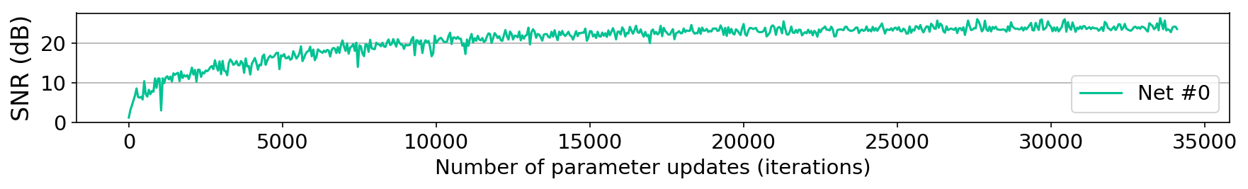
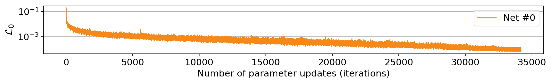
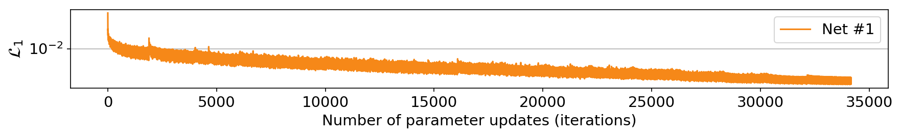
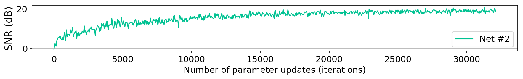
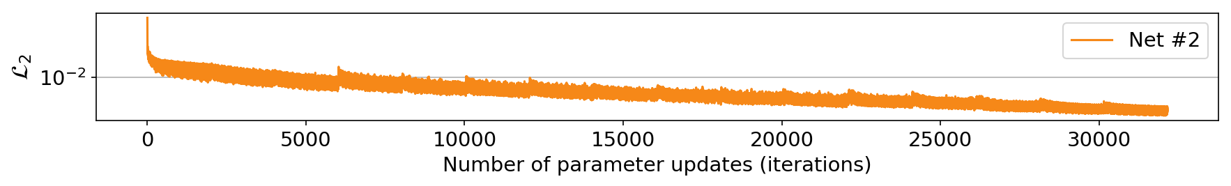
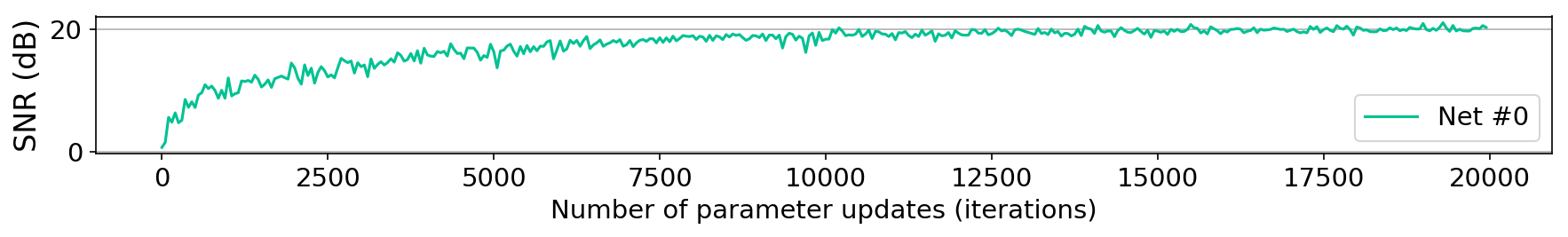
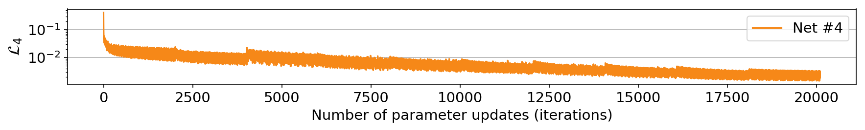
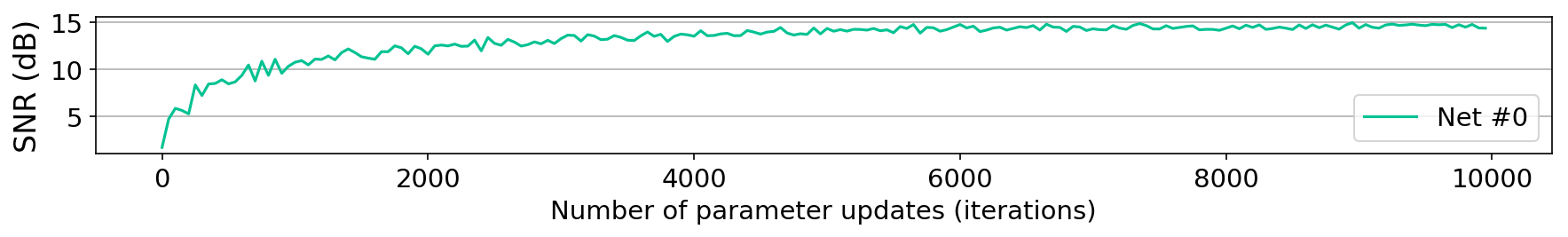
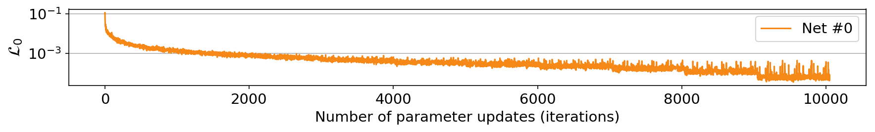
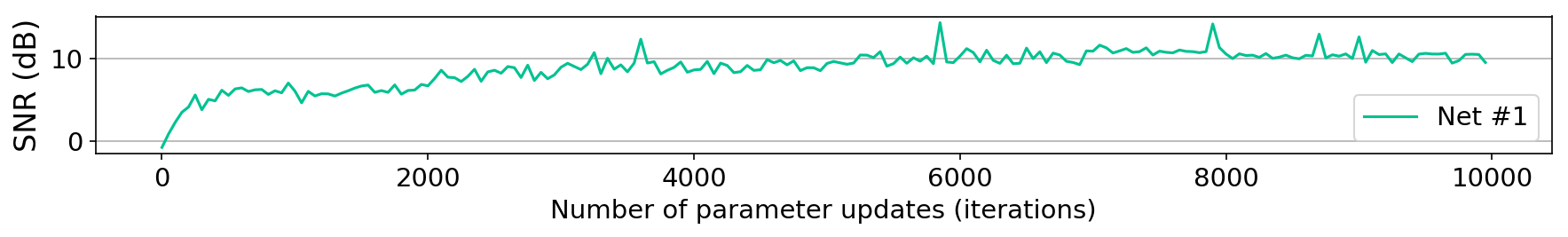
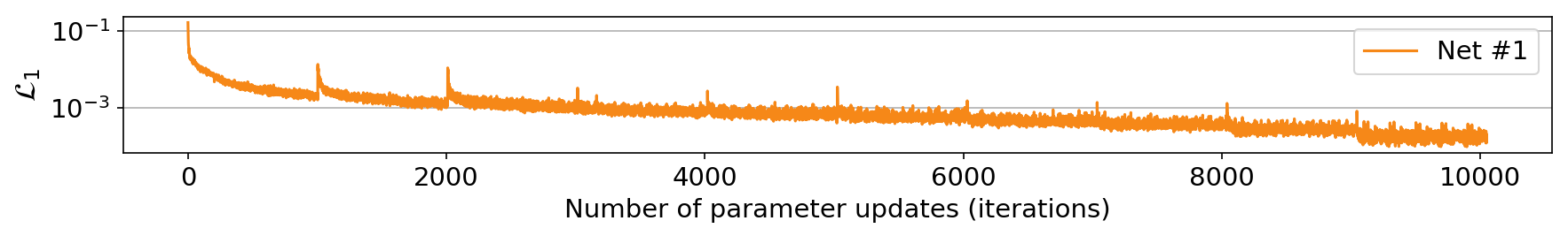
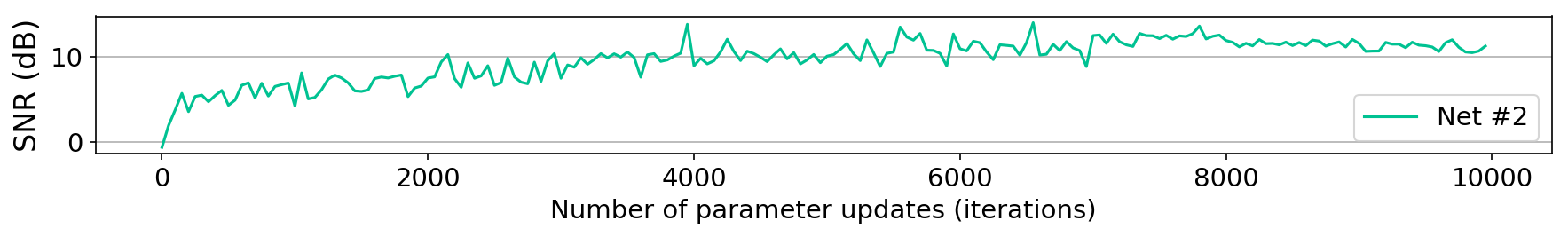
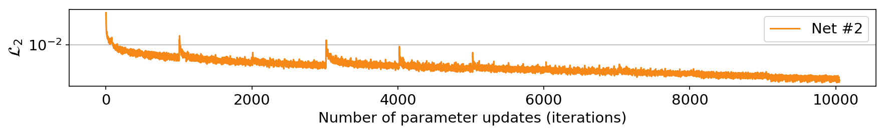
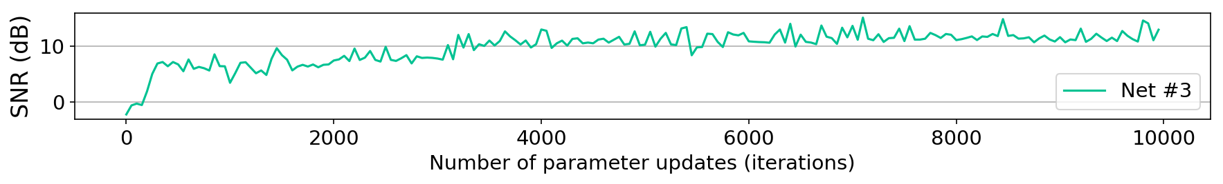
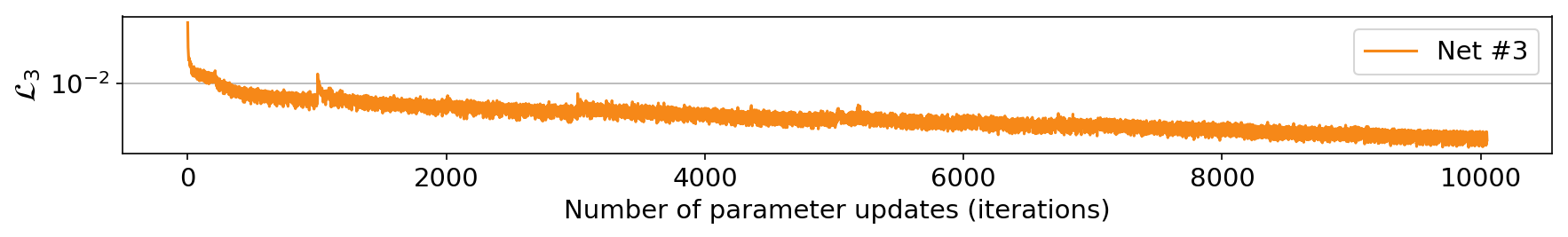
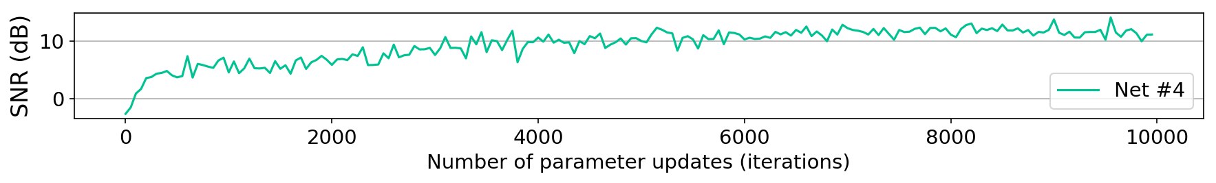
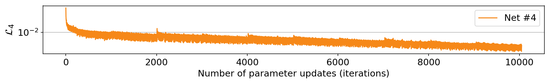
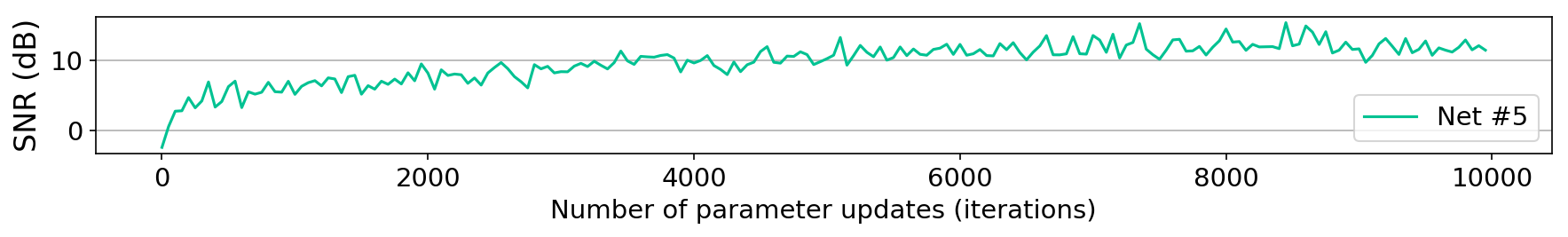
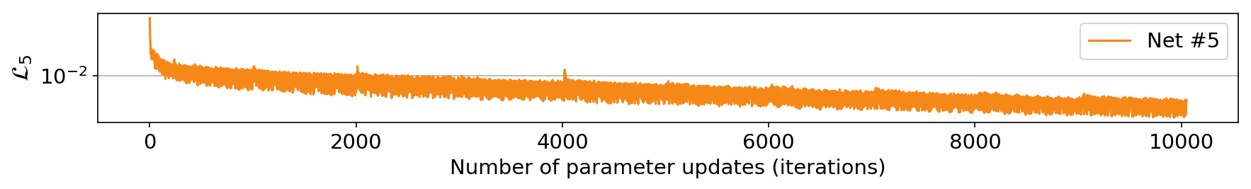
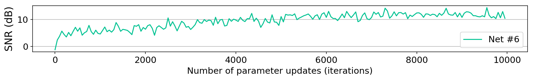
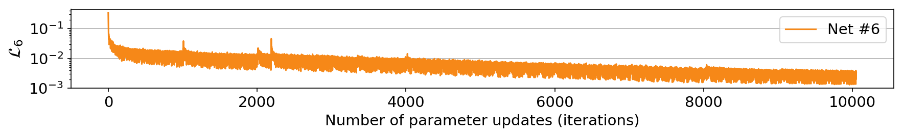
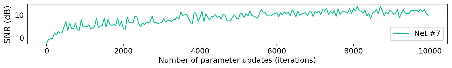
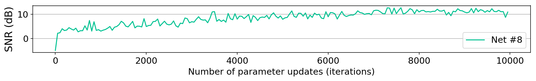
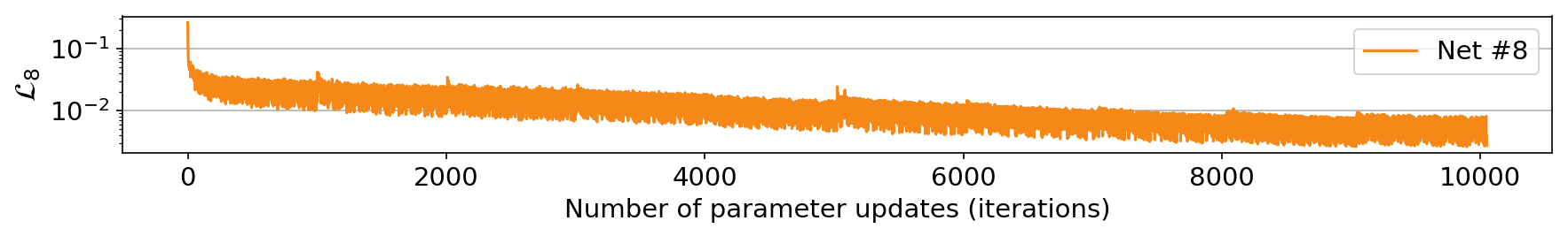
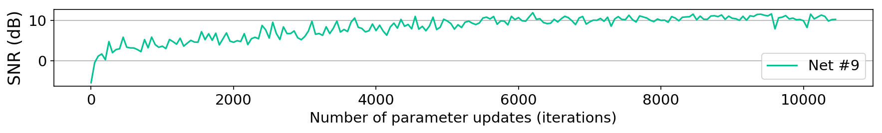
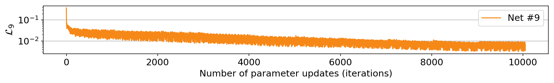
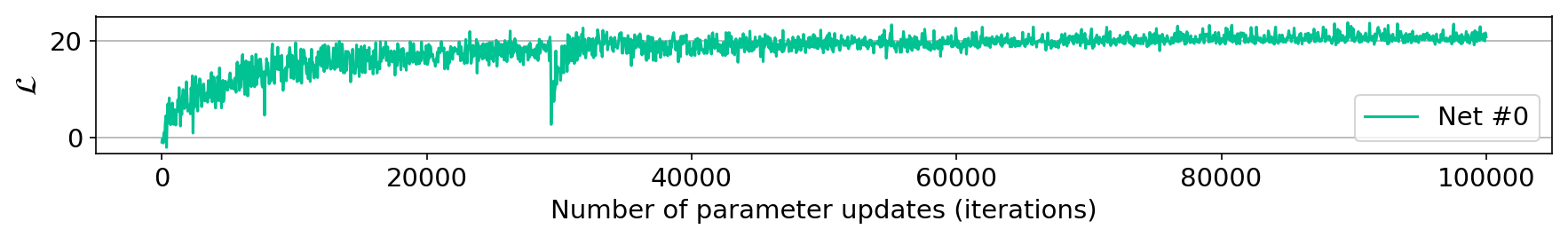
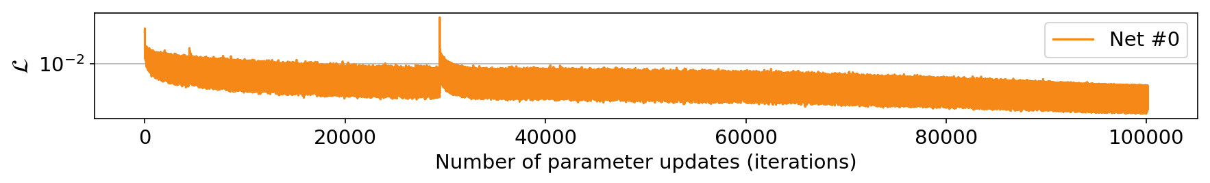
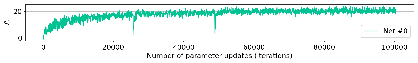
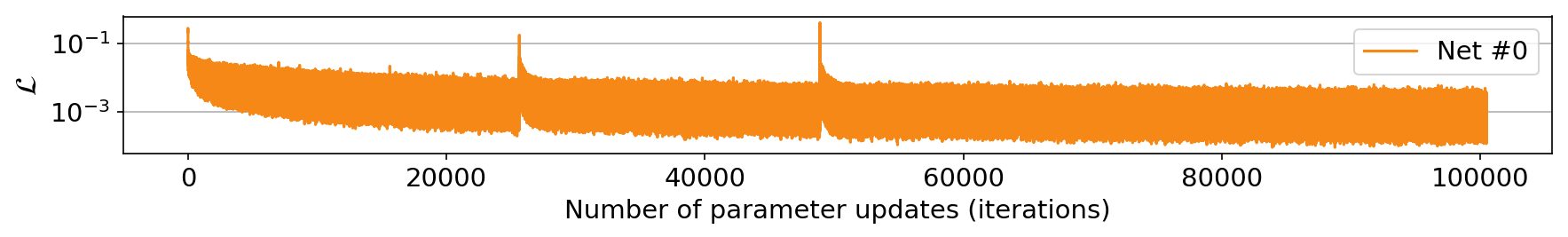
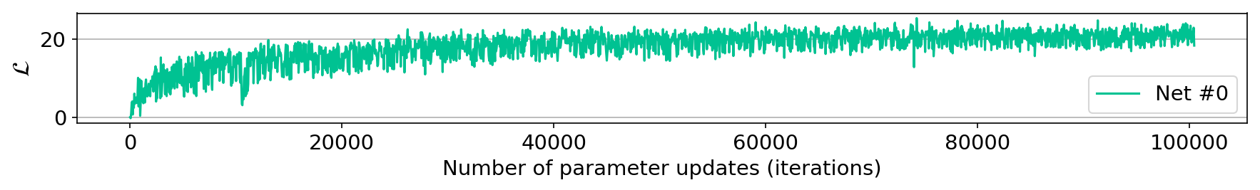
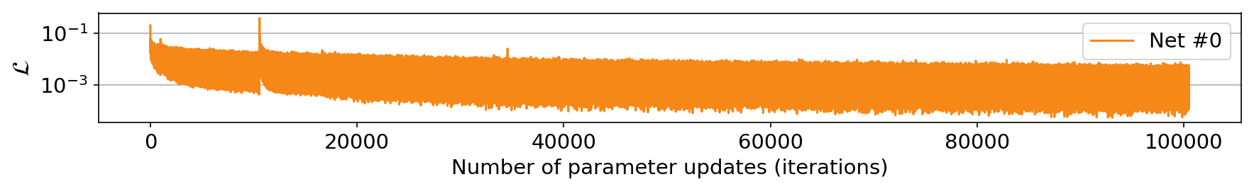
As described earlier and presented in Table 1, the MaxItr variable used in the While condition in line \(8\) of Algorithm 1 is set to \(500\) for all our experiments. Figures 4 \(-\) 6 demonstrate the values of objective function presented in Equation \(\ref{trainCNN-i}\) in orange, and the wavefield correction signal-to-noise ratio (SNR) in blue, evaluated on testing data pairs during training, for experiments with three, five, and ten CNNs, respectively. Note that the SNR curves have not been used to determine when to stop training and they are only depicted for demonstration purposes.

Figures 4a, 4c, and 4e show the wavefield correction SNR for first, second, and third CNN, respectively, in the neural network augmented wave simulator that includes three CNNs. Similarly, Figures 4b, 4d, and 4f depict the training objective values throughout training for first, second, and third CNNs. As it can be seen from objective function curves, the raining heuristic has been effective and the objective function values have a decreasing trend. Note that CNNs has been trained for \(33500\) iterations, on average, with a total of \(100500\) iterations. Several equispaced spikes can be noticed on the objective function value curves. For instance, see the objective value function curve of the third CNN, in Figure 4f, at \(6030, 8040, 10050, \text{and } 12060\) iterations. The mini-batch we use in this experiment is \(10\). Those spikes occur in moments in training when we have started retraining the third CNN, after updating the first and second CNNs. As discussed before, a change in the parameters of the CNNs preceding a CNN causes changes in the input of the later CNN, and consequently the objective function becomes large when starting to retrain the CNNs in later stages again.

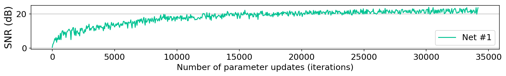
Similar objective function value and SNR curves for other two neural network augmented wave propagators, utilizing five and ten CNNs, can be found in Figures 5 and 6, respectively. First column in Figures 5 and 6, from top to bottom, indicate SNR of wavefield correction obtained by the first to the last CNN, evaluated on testing pairs while training, respectively. The second column of Figures 5 and 6 indicate the objective function value curves throughout optimization of Equation \(\ref{trainCNN-i}\) for training neural network augmented wave propagators, utilizing five and ten CNNs, respectively. In both columns, from top to bottom, the objective function value curves correspond to CNNs from beginning to the end of the learned wave propagators, in order.

We make two main observations from Figures 5 and 6. First, the objective function values indicate overall decreases, validating effectiveness of the introduced heuristic. Also, the spikes on the objective function value curve can be seen, which are correlated with the stages in training when Algorithm 1 revisits a CNN after updating the rest of the CNN parameters. As explained before, spikes are caused by change in parameters of preceding CNNs to a CNN, which in turn alters the input training wavefields of the CNN. Second, due to decrease in iterations per CNN as the number of CNNs increases, the SNR curves converge to a lower value when the number of CNNs increase.

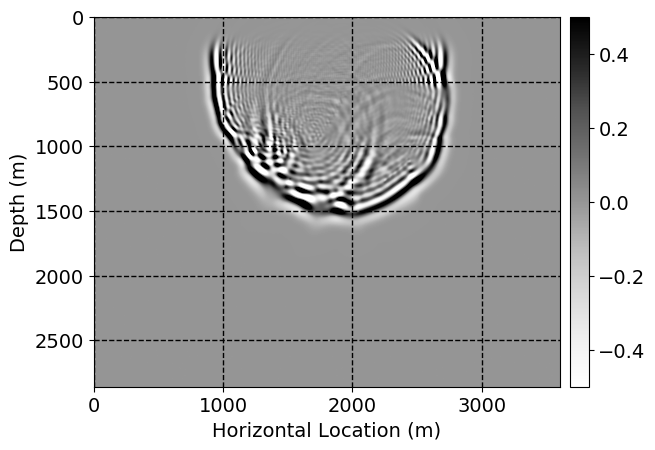
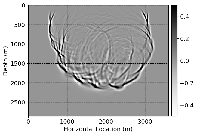
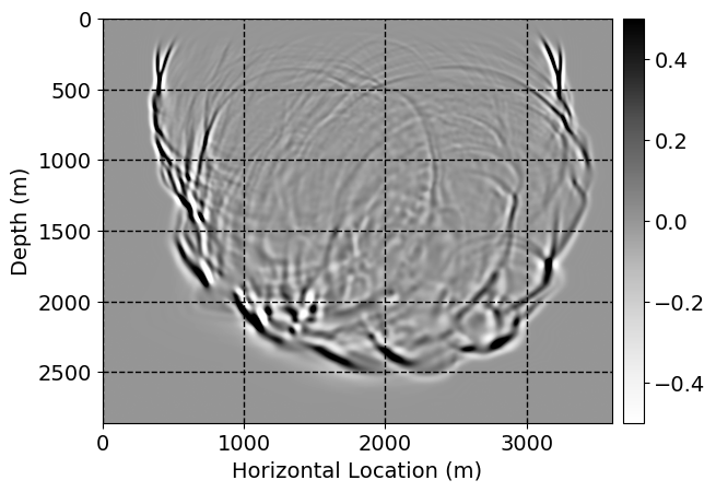
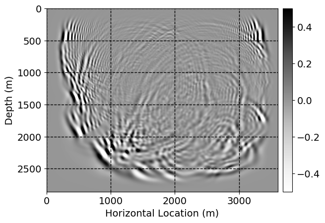
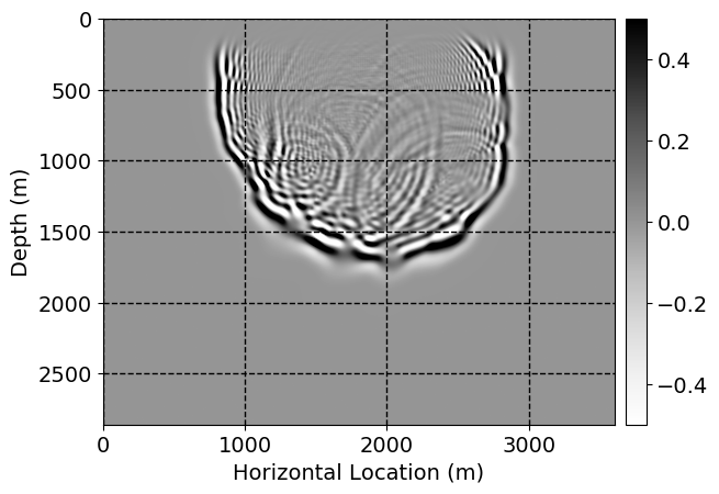
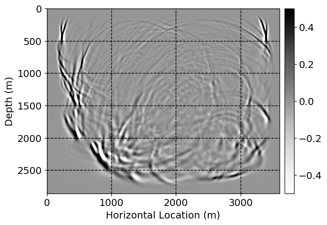
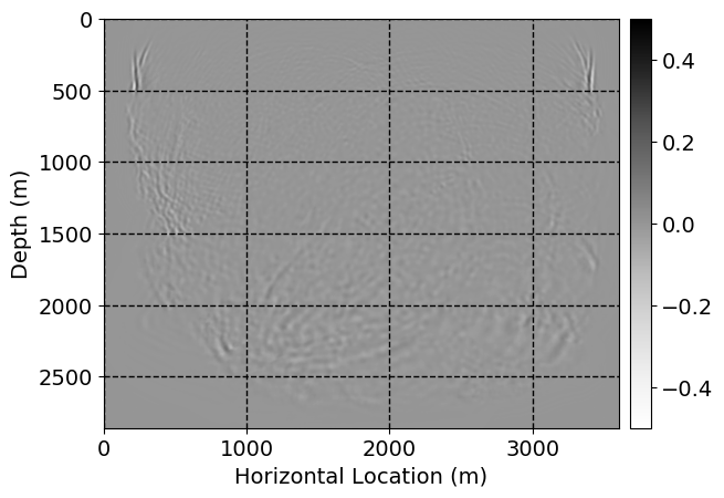
Next, we will demonstrate the the corrected wavefields in three conducted experiments evaluated over one testing shot location. For each experiment, we show the high-fidelity wavefield snapshots, \(\mathbf{u}_{\tau_i}, \ i = 0, 1, \ldots , \lfloor \frac{M-1}{k} \rfloor\), where \(i\) iterates over the CNNs, numerically dispersed low-fidelity wavefields, and the corrected wavefield snapshots by the CNNs. To evaluate the performance of each correction, we also depict the correction error—i.e., difference between the high-fidelity and corrected wavefield snapshots. Figure 7 shows the mentioned wavefield snapshots for the neural network augmented wave simulator with three CNNs. First column shows the high-fidelity wavefields by solving Equation \(\ref{high-fidelity}\), second column depicts low-fidelity simulations by solving Equation \(\ref{low-fidelity}\), third column indicates the result of neural network augmented wavefield simulations, and the fourth column is the learned wave simulation error—i.e., difference between the first and last column in Figure 7. Similarly, Figures 8 \(-\) 10 show the high- and low- fidelity and learned wave simulation wavefield snapshots in the first three columns, in order, for the neural network augmented wave simulator with five and ten CNNs, respectively.

As expected because of the reasons stated before, we observe that the quality of neural network augmented wave-equation simulation degrades as the number of CNNs increases. On the other hands, the high quality of learned wave simulation with few CNNs (see Figure 7) suggests the quality of the simulation with more CNNs might be improved by increasing the number of iterations. As it can be seen in the last column of Figures 9 and 10, the learned wave simulation with ten CNNs has the lowest quality. It can be seen that the learned wave simulation has the least accuracy in direct wave, which happen to be the events with largest amplitudes. Also, it appears that most of the numerical dispersion has been removed, the phase has been recovered, and residual is mostly amplitude differences.

Performance comparison: Single CNN low-to-high-fidelity mapping

In order to evaluate the effectiveness of the proposed method we also train a single CNN similar to our previous attempt to remove numerical dispersion from wavefield snapshots (Siahkoohi et al., 2018, 2019) and compare the result of numerical dispersion removal with the proposed method. To be more precise, for each presented neural network augmented wave-equation simulation experiment, where we use three, five, and ten CNNs, we train a single CNN, \(\mathcal{G}_{\theta}\), with the same architecture as the architecture used in learned wave propagators, in order to remove numerical dispersion from all the low-fidelity wavefield snapshots simulated by solving Equation \(\ref{low-fidelity}\) for \(j\equiv k-1 \ (\bmod \ k)\), on training shot locations. Likewise to previous examples, here we also use half of the available shot locations to simulate training pairs, and the rest is used to evaluate the performance of the trained CNN. The input to \(\mathcal{G}_{\theta}\) during training can be written as follows (compare with Equation \(\ref{inputtoCNN}\)): \[ \begin{equation} \begin{aligned} &\ \mathbf{\tilde{u}}_i = \bar{F}_k (\mathbf{\tilde{u}}_{i-1} ), \quad i = 1, 2, \ldots , \lfloor \frac{M-1}{k} \rfloor, \\ &\ \mathbf{\tilde{u}}_0 = \bar{F}_k(\mathbf{q}), \\ \end{aligned} \label{inputtoSingleCNN} \end{equation} \] The desired output for the mentioned CNN is the high-fidelity wavefield snapshots simulated on training shot locations, \(\mathbf{u}_{\tau_i}^{(p)}, \ p = 0,1, \ldots , n-1, \ i = 0, 1, \ldots , \lfloor \frac{M-1}{k} \rfloor\). The objective function for the mentioned CNN can be represented as follows: \[ \begin{equation} \begin{split} \mathcal{L} = \frac{1}{n (\lfloor \frac{M-1}{k} \rfloor + 1)} \sum_{i=0}^{\lfloor \frac{M-1}{k} \rfloor} \sum_{p=0}^{n-1} \left \| \mathcal{G}_{\theta}(\mathbf{\tilde{u}}_i^{(p)}) - \mathbf{u}_{\tau_i}^{(p)} \right \|_1. \\ \end{split} \label{trainCNN-single} \end{equation} \] We minimize objective function \(\ref{trainCNN-single}\) over \(\theta\) with Adam optimizes, using the same maximum number of iterations as before, this time by combining all the training pairs associated with different CNNs in the learned wavefield simulation example. As mentioned before, in order to compare with the proposed method, we minimize objective function \(\ref{trainCNN-single}\) over three different set of input-output pairs, each corresponding to our presented experiments with varying number of CNNs. Table 2 summarizes the total number of iterations, training pairs, training time, and number of tunable parameters for three different cases, which differ in number of timesteps which we choose to correct the numerical dispersion. This selected timesteps are associated with the timesteps that the CNNs operated on, in our three previous examples.

# Timesteps to correct	Iterations	Pairs per CNN	Time	Param. count
\(3\)	\(100500\)	\(603\)	\(13.85\) hours	\(11383424\)
\(5\)	\(100500\)	\(1005\)	\(13.96\) hours	\(11383424\)
\(10\)	\(100500\)	\(2010\)	\(14.56\) hours	\(11383424\)

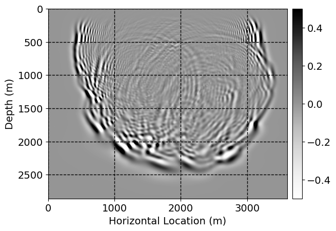
The slight difference in runtime among three different cases provided in Table 2 is partly due to different number of training pairs needed to be generated. Figure 11 depicts the wavefield snapshot correction SNR curves, evaluated on testing pairs while training, and the value of objective function \(\ref{trainCNN-single}\), in single CNN low-to-high-fidelity mapping experiment, as a function of number of iterations. Figures 11a, 11c, and 11e show the SNR curves, when we trained the CNN on wavefield snapshots correspond to three, five, and ten, timesteps, respectively. Similarly, Figures 11b, 11d, and 11f depict the training objective function value (Equation \(\ref{trainCNN-single}\)), when the CNN is trained on wavefield snapshots correspond to three, five, and ten, timesteps, respectively. SNR curves depicted in first column of Figure 11 show the evolution of wavefield correction SNR evaluated on randomly selected testing wavefield wavefields form the wavefield snapshots combined from different timesteps. Therefore, Figures 11a, 11c, and 11e indicate that the three different CNNs converge to a wavefield correction SNR around \(20\) dB, regardless of number of timesteps they are correcting for. Although this does not suggest that the performance will stay the same as we increase the number of timesteps needed to be corrected. By comparing Figure 11a with first column of Figure 4 (SNR curves for neural network augmented wave-equation simulation with three CNNs), we observe that, on average the two methods are performing equally well.

Finally, we will show the wavefield corrected by the single CNN low-to-high-fidelity mapping method, for comparison with our proposed method. Figures 12 and 13 indicate the corrected wavefields, for cases where three and five timesteps need to be corrected. Figures 14 and 15 demonstrate the corrected wavefields, for the case where ten timesteps need to be corrected, in two parts. In Figures 12 \(-\) 15, the first, second, third, and fourth columns depict the high-fidelity and low fidelity wavefield snapshots, corrected low-fidelity wavefield snapshots, and the error in numerical dispersion removal, respectively. In each columns, from top to bottom, the simulation time increases.

For comparison between our proposed method and single CNN low-to-high-fidelity mapping, compare Figures 7 with 12, 8 with 13, 9 with 14, 10 with 15. As it can be seen, the single CNN low-to-high-fidelity mapping method maintains the quality of its performance when the number of timesteps that need to be corrected increases. On the other hand, as the number of CNNs in neural network augmented wave-equation simulation increases, the performance drops, by keeping the maximum number of iterations fixed. Also, by comparing Tables 1 and 2, we observe that the training time needed for single CNN low-to-high-fidelity mapping, when number of timesteps needed to be corrected increases, for fixed number of maximum iterations, grows very slowly compared to the training time required for neural network augmented wave-equation simulation.

Conclusions

Our numerical experiments demonstrate that, given suitable training data, the well-trained neural network augmented wave-equation simulator is capable of approximating wavefield snapshots simulated by high-fidelity simulation. In this work, as a proxy of inaccurate physics, we simulate wave-equation with finite-difference method, using a poor discretization of Laplacian. Although not computationally favorable to high-fidelity wave simulation, we showed that the learned wave simulator deals with inaccurate physics. An important observation we made is that training time of the proposed method gets quickly very long and to achieve high accuracy, it may not be possible to utilize too many CNNs. On the other hand, training time required for the single CNN low-to-high-fidelity mapping experiments, conducted for the sake of comparison, grows very slowly as the number of timesteps to be corrected increases. In future, we intend to initialize the CNN parameters in the proposed method with the parameters of a CNN trained by the single CNN low-to-high-fidelity mapping algorithm. The initialization may significantly reduce the training time needed for the neural network augmented wave-equation simulation method, and may give the chance to fine-tune the CNNs to the specific timestep that each CNN is assigned to correct.

Acknowledgments

The authors thank Xiaowei Hu for his open-access repository⁵ on GitHub. Our software implementation built on this work.

---

1. https://www.tensorflow.org/↩

2. https://www.devitoproject.org/↩

3. https://odlgroup.github.io/odl/↩

4. https://github.com/alisiahkoohi/NN-augmented-wave-sim↩

5. https://github.com/xhujoy/CycleGAN-tensorflow↩