Ultra-low memory seismic inversion with randomized trace estimation

Mathias Louboutin¹, Felix J. Herrmann^1,2
1 School of Earth and Atmospheric Sciences, Georgia Institute of Technology
² School of Computational Science and Engineering, Georgia Institute of Technology

Summary:

Inspired by recent work on extended image volumes that lays the ground for randomized probing of extremely large seismic wavefield matrices, we present a memory frugal and computationally efficient inversion methodology that uses techniques from randomized linear algebra. By means of a carefully selected realistic synthetic example, we demonstrate that we are capable of achieving competitive inversion results at a fraction of the memory cost of conventional full-waveform inversion with limited computational overhead. By exchanging memory for negligible computational overhead, we open with the presented technology the door towards the use of low-memory accelerators such as GPUs.

Introduction

Wave-equation based seismic inversion has resulted in tremendous improvements in subsurface imaging over the past decade. However, the computational cost, and above-all memory cost, of these methods remains extremely high limiting their widespread adaptation. These memory costs stem from the requirement of the adjoint-state method (Lions, 1971, Tarantola (1984)) to store (in memory, on disk, possibly compressed) the complete time history of the forward modeled wavefield prior to on-the-fly crosscorrelation with the time-reversed or adjoint wavefield. Unfortunately, the need to store these forward wavefields for each source may require allocation of up to terabytes of memory during high-frequency 3-D imaging. To tackle this memory requirement and to open the way to the use of low-memory accelerators such as GPUs, different methods have been proposed that balance memory usage with computational overhead to reduce the memory footprint. One of the earliest methods in this area is optimal checkpointing (Griewank and Walther, 2000, Symes (2007)), which has recently been extended to include wavefield compression (N. Kukreja et al., 2020). Given available memory, optimal checkpointing reduces storage needs at the expense of having to recompute the forward wavefield. While the resulting memory savings can be significant, the computational overhead can be high (up to tens of extra wave-equations). Alternatively, by relying on time-reversibility of the (attenuation-free) wave-equation, McMechan (1983), Mittet (1994), Raknes and Weibull (2016) proposed an approach where the forward wavefield is reconstructed during back propagation from values stored on the boundary. Even though these approaches have been applied successfully in practice, their implementation becomes elaborate especially in situations of complex wave physics such as in elastic or transverse-tilted anisotropic media.

Aside from the aforementioned methods that are in principle error free, except perhaps for methods that involve lossy compression, approximate methods have also been proposed to reduce the memory imprint of gradient calculations for wave-equation based imaging. The rationale behind these approximations is that by giving up accuracy one may gain computationally and/or memorywise. This was, for example, the main idea behind imaging with phase-encoded sources (Romero et al., 2000, Krebs et al. (2009), Moghaddam et al. (2013), Haber et al. (2015), Leeuwen and Herrmann (2013)). According to insights from stochastic optimization, there are strong arguments that accurate gradients are indeed unnecessary especially at the beginning of the optimization and as long as the approximate gradient equals the true gradient in expectation (M. P. Friedlander and Schmidt, 2012). We make use of this fundamental observation and propose a new, simple to implement, alternative formulation that allows for approximate gradient calculations with a significantly reduced memory imprint. At first sight, our method may be somewhat reminiscent of memory-reducing methods based on the Fourier transform, which compute the Fourier transform either on the fly (Sirgue et al., 2010, P. A. Witte et al. (2019)) or in windows (Nihei and Li, 2007). Our method is based on a randomized trace estimation technique instead. Like Fourier methods, which derive their advantage from computing the gradient for a relatively small number of Fourier modes, the proposed randomized algorithm collects compressed data during forward propagation. This leads to significant memory savings at a manageable computational overhead (similar if not cheaper than checkpointing (P. A. Witte et al., 2020)). However, compared to optimal checkpointing and boundary methods, Fourier techniques involve inaccurate gradients that may result in coherent artifacts during the inversion. Contrarily, our randomized linear algebra based method produces incoherent artifacts, easily handled by regularizations methods, with a computational overhead of at least half of that of Fourier methods thanks to real-valued arithmetic.

Inspired by recent work on randomized linear algebra for seismic inversion (Leeuwen et al., 2017, M. Yang et al. (2021)), we propose an alternative method based on random trace estimation. Unlike direct time subsampling (Louboutin and Herrmann, 2015), randomized trace estimation involves matrix probing with random vectors (Avron and Toledo, 2011, Meyer et al. (2020)) (vectors with random \(\pm 1\)’s or Gaussian vectors) frequently employed by randomized algorithms, such as the randomized SVD (Halko et al., 2011). These probings are computationally efficient because they only involve actions of the matrix on a small number of random vectors. This allows us to compress the time axes during forward propagation, greatly reducing memory usage in a computationally efficient way, yielding gradient calculations with a controllable error.

Our contributions are organized as follows. First, we introduce randomized trace estimation including a recently proposed orthogonalization step that improves its performance and accuracy. Next, we show that gradients calculated with the adjoint-state method for wave-equation based inversion can be approximated by random trace estimation. Compared to conventional gradient calculations, the approximated gradient leads to significant memory reductions and faster computation of certain imaging conditions. To further justify the proposed algorithm, we discuss how its computational and memory requirements compare to existing methods. We conclude by illustrating the advocacy of the proposed method on a 2D synthetic full-waveform inversion example.

Methodology

In this section, we briefly lay out the key components of our seismic inversion method that requires significantly less memory. We start by introducing stochastic estimates for the trace of a matrix, followed by how these estimates can be used to approximate the gradient of a time-domain formulation of the adjoint state method for the wave-equation. We conclude by providing estimates of memory use of the proposed method and how it compares to other memory reducing methods.

Randomized trace estimation

To address memory pressure of data-intensive applications, a new generation of randomized algorithms have been proposed. Contrary to classical deterministic techniques that aim for maximal accuracy, these methods are stochastic in nature and provide answers with a controllable error. Examples of these techniques are the randomized SVD (Halko et al., 2011, M. Yang et al. (2021)) and randomized trace estimation (Avron, Meyer et al., 2020). The latter was used to justify wave-equation inversions with random phase encoding (Haber et al., 2015, Leeuwen and Herrmann (2013)). In this work, we also rely on randomized trace estimation but now to reduce the memory imprint of wave-equation based inversion. At its heart, randomized trace estimation (Avron and Toledo, 2011, Meyer et al. (2020)) derives from the following approximation of the identity \(\mathbf{I}\): \[ \begin{equation} \begin{aligned} \operatorname{tr}(\mathbf{A}) &=\operatorname{tr}\left(\mathbf{A} \mathbb{E}\left[\mathbf{z} \mathbf{z}^{\top}\right]\right) =\mathbb{E}\left[\operatorname{tr}\left(\mathbf{A} \mathbf{z} \mathbf{z}^{\top}\right)\right]\\ &= \mathbb{E}\left[\mathbf{z}^{\top} \mathbf{A} \mathbf{z}\right] \approx \frac{1}{r}\sum_{i=1}^r\left[\mathbf{z}^{\top}_i \mathbf{A} \mathbf{z}_i\right]= \frac{1}{r}\operatorname{tr}\left(\mathbf{Z}^\top \mathbf{A}\mathbf{Z}\right) \end{aligned} \label{randomtrace} \end{equation} \] where the \(\mathbf{z}_i\)’s are the random probing vectors for which \(\mathbb{E}(\mathbf{z}^{\top}\mathbf{z})=1\) and \(\mathbb{E}\) is the stochastic expectation operator. The above estimator is unbiased (exact in expectation) and converges to the true trace of the matrix \(\mathbf{A}\), i.e. \(\operatorname{tr}(A)=\sum_i \mathbf{A}_{ii}\), with an error that decays with \(r\) and without access to the entries of \(\mathbf{A}\). Only actions of \(\mathbf{A}\) on the probing vectors are needed and we will exploit this property and the factored form of the matrix \(\mathbf{A}\) in gradient calculations for wave-equation based inversion. Motivated by recent work (Meyer et al., 2020, Graff-Kray et al. (2017)) we will also employ a partial qr factorization (Trefethen and Bau III, 1997) that approximates the range of the matrix \(\mathbf{A}\)—i.e., we approximate the trace with probing vectors \(\begin{bmatrix}\mathbf{Q},\thicksim\end{bmatrix} = \operatorname{qr}(\mathbf{A}\mathbf{Z})\) where \(\mathbf{Z}\) is a Rademacher random matrix of \(\pm 1\).

Approximate gradient calculations

While one may argue that inaccurate gradients need to be avoided at all times, approximations to the gradient are actually quite common. For instance, wave-equation based inversion with phase-encoded sources derives from a similar approximation but this time on the data misfit objective. Haber et al. (2015) showed that this type of approximate inversion is an instance of random trace estimation. In addition, possible artifacts can easily be removed by adding regularization, e.g. by imposing the TV-norm constraint on the model (Esser et al., 2018, Peters et al. (2018)) or by including curvelet-domain sparsity constraints on Gauss-Newton updates (X. Li et al., 2016). Let us consider the standard adjoint-state FWI problem, which aims to minimize the misfit between recorded field data and numerically modeled synthetic data (Lions, 1971, Tarantola (1984), Virieux and Operto (2009), Louboutin et al. (2017), Louboutin et al. (2018)). In its simplest form, the data misfit objective for this problem reads \[ \begin{equation} \underset{\mathbf{m}}{\operatorname{minimize}} \ \frac{1}{2} ||\mathbf{F}(\mathbf{m}; \mathbf{q}) - \mathbf{d}_{\text{obs}} ||_2^2 \label{adj} \end{equation} \] where \(\mathbf{m}\) is a vector with the unknown physical model parameter (squared slowness in the isotropic acoustic case), \(\mathbf{q}\) the sources, \(\mathbf{d}_{\text{obs}}\) the observed data and \(\mathbf{F}\) the forward modeling operator. This data misfit is typically minimized with gradient-based optimization methods such as gradient descent (Plessix, 2006) or Gauss-Newton (X. Li et al., 2016). While the presented approach carries over to arbitrary complex wave physics, we derive our memory reduced gradient approximation for the isotropic acoustic case where the gradient for a single source \(\delta\mathbf{m}\) can be written as \[ \begin{equation} \delta\mathbf{m} = \sum_t \mathbf{\ddot{u}}[t] \mathbf{v}[t] \label{iccc} \end{equation} \] where \(\mathbf{u}[t], \mathbf{v}[t]\) are the vectorized (along space) full-space forward and adjoint solutions of the forward and adjoint wave-equation at time index \(t\). The symbol \(\ddot{}\) represents second-order time derivative. To arrive at a form where randomized trace estimation can be used, we write the above zero-lag crosscorrelation over time as the trace of the outer product for each space index \(\mathbf{x}\) separately. By using the dot product property, \(\sum \mathbf{x}_i \mathbf{y}_i=\mathbf{x}^\top\mathbf{y}=\operatorname{tr}(\mathbf{x}\mathbf{y}^\top)\), in combination with Equation \(\ref{randomtrace}\), we approximate the gradient via random-trace estimation—i.e., \[ \begin{equation} \begin{split} \delta\mathbf{m}[\mathbf{x}] = \operatorname{tr}\left(\mathbf{\ddot{u}}[t, \mathbf{x}]\mathbf{v}[t, \mathbf{x}]^\top\right) \approx \frac{1}{r} \operatorname{tr}\left((\mathbf{Q}^\top \mathbf{\ddot{u}}[\mathbf{x}]) (\mathbf{v}[\mathbf{x}]^\top \mathbf{Q})\right) \\ \end{split} \label{optr} \end{equation} \] where parenthesis were added to show that the matrix-vector products between the wavefields and the probing matrix \(\mathbf{Q}\) can be computed independently. We use this property to arrive at our proposed ultra-low memory unbiased approximation of the gradient summarized in Algorithm 1 below. This algorithm runs for each space index with the same probing matrix \(\mathbf{Q}\). Instead of storing the wavefield during the forward pass, e.g. via checkpointing, the sum of the probed (with \(\mathbf{Q}^\top\)) wavefield is for each space index accumulated (line 2) in the variable \(\overline{\mathbf{u}}[\mathbf{x}]\). Because of the probing, we only need to store \(N\times r\) with \(r\ll n_t\) samples in \(\overline{\mathbf{u}}\) instead of \(N\times n_t\) with \(n_t\) the number of timesteps. As we will show, \(r\) can be very small compared to \(n_t\), leading to significant memory savings. Similarly, during the back propagation pass (lines 4-7), we accumulate for each spatial index \(\overline{\mathbf{v}}\). After finishing the back propagation iterations, the gradient is calculated by computing the trace of the outer product of the accumulated probed wavefields (line 8). To avoid forming an unnecessarily large matrix for the outer product in line 8, we simply compute the sum over the probing size of the pointwise product of \(\overline{\mathbf{u}}\) and \(\overline{\mathbf{v}}\) in practice. Before deriving a practical scheme for FWI based on this probing scheme, let us first discuss its memory use and how it compares to other known approaches to reduce the memory imprint of wave-equation based inversion.

0. for t=2:nt-1            # forward propagation
1.    \(\mathbf{u}[t+1] = f(\mathbf{u}[t], \mathbf{u}[t-1], \mathbf{m}, \mathbf{q}[t])\)
2.    \(\overline{\mathbf{u}}[\mathbf{x}, \cdot] \pluseq \mathbf{Q}[\cdot, t]^\top \mathbf{\ddot{u}}[t, \mathbf{x}]\)
3. end for
4. for t=nt:-1:1           # back propagation
5.    \(\mathbf{v}[t-1] = f^\top(\mathbf{v}[t], \mathbf{v}[t+1], \mathbf{m}, \delta \mathbf{d}[t])\)
6.    \(\overline{\mathbf{v}}[\cdot, \mathbf{x}] \pluseq \mathbf{v}[t, \mathbf{x}] \mathbf{Q}[\cdot, t]\)
7. end for
8. output: \(\frac{1}{r}\operatorname{tr}(\overline{\mathbf{u}}\, \overline{\mathbf{v}}^\top)\)

Memory estimates

From Equation \(\ref{optr}\), we can easily estimate the memory imprint of our method compared to conventional FWI. For completeness, we also consider other mainstream low memory methods: optimal checkpointing (Griewank and Walther, 2000, Symes (2007), N. Kukreja et al. (2020)), boundary methods (McMechan, 1983, Mittet (1994), Raknes and Weibull (2016)), and DFT methods (Nihei and Li, 2007, Sirgue et al. (2010), P. A. Witte et al. (2019)). This memory overview generalizes to other wave-equations and imaging conditions easily as our method generalizes to any time-domain adjoint-state method. We estimate the memory requirements for a three-dimensional domain with \(N=N_x \times N_y \times N_z\) grid points and \(n_t\) time steps. Conventional FWI requires storing the full time-space forward wavefield to compute the gradient. This requirement leads to a memory requirement of \(N\times n_t\) floating point values. Our method, on the other hand, for \(r\) probing vectors (i.e \(\mathbf{Q} \in \mathbb{R}^{n_t \times r}\)), requires only \(N\times r\) floating point values during each of the forward and backward passes for a total of \(2\times N\times r\) values. The memory reduction factor is, therefore, \(\frac{n_t}{2 r}\). This memory reduction is similar to computing the gradient with \(\frac{r}{2}\) Fourier modes. We summarize the memory usage compared to other state-of-the-art algorithms in table 1.

	FWI	DFT	Probing	Optimal checkpointing	Boundary reconstruction
Compute	0	\(\mathcal{O}(2r)\times n_t \times N\)	\(\mathcal{O}(r)\times n_t \times N\)	\(\mathcal{O}(log(n_t))\times N \times n_t\)	\(n_t \times N\)
Memory	\(N \times n_t \)	\(2r\times N\)	\(r \times N\)	\(\mathcal{O}(10) \times N\)	\(n_t \times N^{\frac{2}{3}}\)

It is worth noting that unlike the other methods in the table, boundary reconstruction methods tend to have stability issues for more complex physics, in particular with physical attenuation making it ill-suited for real-world applications. As stated in the introduction, our method closely follows the computational and memory cost of Fourier methods by a factor of two related to real versus complex arithmetic. We also show that unlike checkpointing or boundary methods, neither the memory nor computational overhead depends on the number of time steps, therefore our method offers improved scalability.

Imaging conditions

Aside from these clear advantages regarding memory use, the proposed approximation scheme also has computational advantages when imposing more elaborate imaging conditions such as the inverse scattering imaging condition (Whitmore and Crawley, 2012, P. Witte et al. (2017)) for RTM or wavefield separation (Liu et al., 2011) for FWI. In most cases, these imaging condition can be expressed as linear operators that only act on the spatial dimensions of the wavefields and not along time. Because these operators are linear, we can factor these operators out and directly apply them to the probed wavefields consisting of r reduced time steps rather than to every time steps with \(n_t\gg r\). We can achieve this by making use of the following identity (the same applies to \(\mathbf{v}\)): \[ \begin{equation} \mathbf{Q}^\top \left(\mathbf{D}_x \mathbf{u}[\cdot,\mathbf{x}]\right) = \mathbf{D}_x \left(\mathbf{Q}^\top \mathbf{u}[\cdot,\mathbf{x}]\right), \label{commute} \end{equation} \] which holds as long as the linear imaging condition only acts along the space directions and not along time. Because \(r\ll n_t\) this can lead to significant computational savings especially in the common situation where imposing imaging conditions becomes almost as expensive as solving the wave-equation itself.

Choice of the probing matrix \(\mathbf{Q}\)

While strictly random, e.g. random \(\pm 1\) as in Rademacher or Gaussians (Avron and Toledo, 2011) an extra orthogonalization step (via a qr factorization on random probings \(\mathbf{A}\mathbf{Z}\)) allows us to capture the range of \(\mathbf{A}\) (Meyer et al., 2020, Graff-Kray et al. (2017)), which leads faster decay of the error as a function of \(r\). This error in the gradient is due to “cross talk”—i.e. \(\mathbf{Z}\mathbf{Z}^\top\ne\mathbf{I}\). Unfortunately, we do not have easy access to \(\mathbf{A}\) during the approximate gradient calculations outlined in Algorithm 1. Moreover, orthogonalizing each spatial gridpoint separately would be computationally infeasible. Despite these complications, we argue that we can still get a reasonable approximation of the range by random probing the observed data organized as a matrix for each source experiment—i.e., we have \[ \begin{equation} \begin{bmatrix}\mathbf{Q},\thicksim\end{bmatrix} = \operatorname{qr}(\mathbf{A}\mathbf{Z}) \quad\text{with}\quad \mathbf{A}=\mathbf{D}_{\text{obs}}\mathbf{D}_{\text{obs}}^\top \label{QR} \end{equation} \] 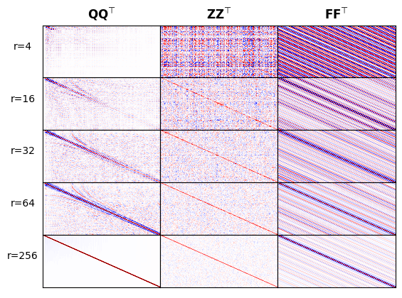where the observed data vector \(\mathbf{d}_{\text{obs}}\) for each shot is shaped into a matrix along the time and lumped together receiver coordinates. Since observed data contains information on the temporal characteristics of the wavefields, we argue that this outer product can serve as a proxy for the time characteristics of the wavefield everywhere. In Figure 1, we demonstrate the benefits of the additional orthogonalization step by comparing the outer products of the Rademacher probing matrix \(\mathbf{Z}\), the restricted Fourier matrix \(\mathbf{F}\), and orthogonalized probing vectors \(\mathbf{Q}\) as a function of increasing \(r\). The following observations can be made. First, as expected the “cross-talk”, i.e. amplitudes away from the diagonal, becomes smaller when \(r\) increases, which is to be expected for all cases. However, we observe also that the outer product converges faster to the identity for both the Rademacher and qr factored case while coherent artifact remain with Fourier due to the truncation. Second, because of the orthogonalization the artifacts for the outer product of \(\mathbf{Q}\) are much smaller and this should improve the accuracy of the gradient at the expense of a relatively minor cost of carrying our a qr factorization for each shot record. Finally, compared to the Fourier basis, in combination with source spectrum informed frequency sampling, our probing factors are informed by estimates of the range of the sample covariance kernel spanned by the traces in each shot record.

Example

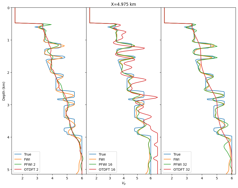
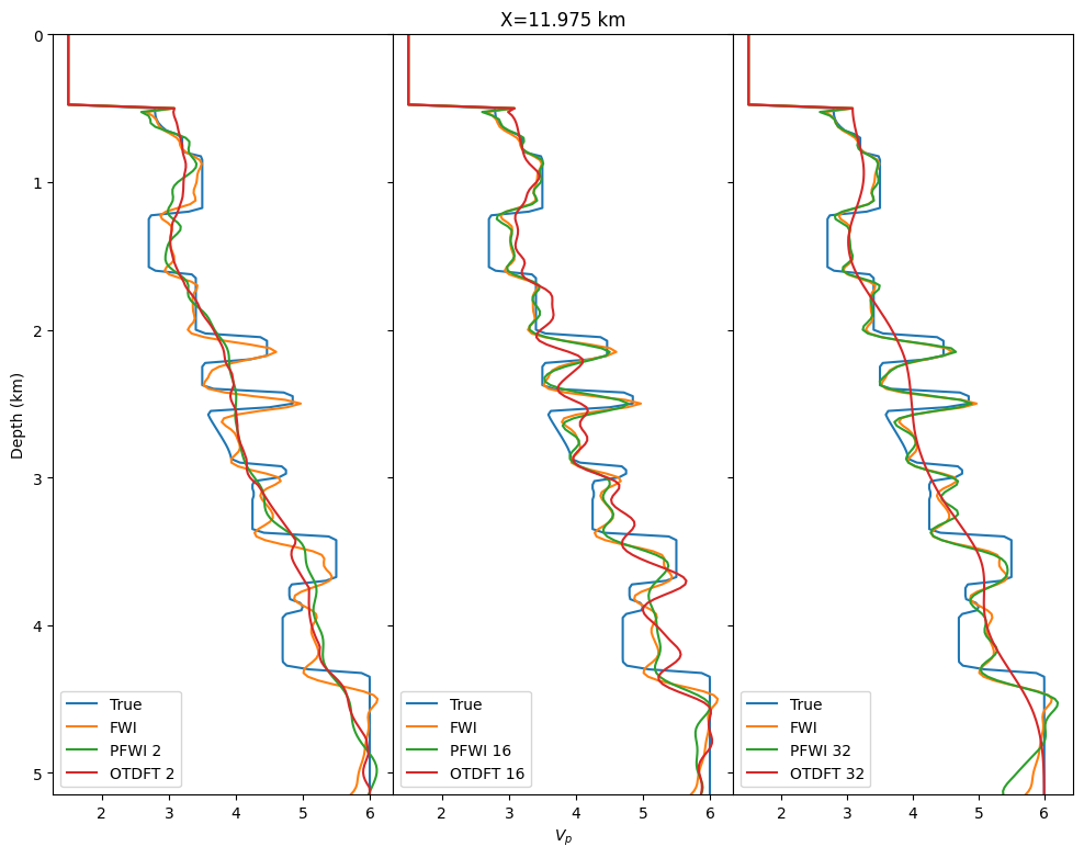
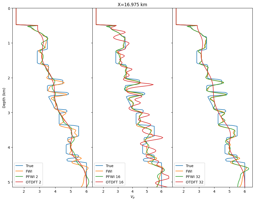
We illustrate our method on the 2D overthrust model and compare our inversion results to conventional FWI and on-the-fly DFT (Sirgue et al., 2010, P. A. Witte et al. (2019)). We consider a \(20\)km by \(5\)km 2D slice of the well-known overthrust model. The dataset consists of \(97\) sources \(200\)m apart at \(50\)m depth. Each shot contains between \(127\) and \(241\) ocean bottom nodes \(50\)m apart at \(500\)m depth for a maximum offset of \(6\)km. The data is modeled with an \(8\)Hz Ricker wavelet and \(3\)sec recording. We show the true model and the initial background model with the inversion results in Figure 2. We ran \(20\) iterations of Spectral Projected Gradient (SPG, gradient descent with box constraints (Schmidt et al., 2009)) with \(20\) randomly selected shots per iteration (Aravkin et al., 2012) in all cases. We can clearly see from Figure 2 that our probed gradient allows the inversion to carry towards a good velocity estimate. As theoretically expected, for few probing vectors, we do not converge since our approximation is not accurate enough. However, we start to obtain a result comparable to the true model with as few as \(16\) probing vectors. Additionally, this result could easily be improved by adding constraints as regularization (Esser et al., 2018, Peters et al. (2018)). On the other hand, we can also see in Figure 2 that for an equivalent memory cost, on-the-fly DFT fails to converge to an acceptable result for any number of frequencies, most likely due to the coherent artifacts that stem from the DFT. These results could also be improved with constraints or with a better choice of selected frequencies. We finally compare the three vertical traces highlighted in black to detail the accuracy of the inverted velocity plotted in Figure 2. These traces show that our probed inversion result is in the vicinity of results obtained with standard FWI, which itself is close to the true model.

Our implementation and examples are open sourced at TimeProbeSeismic.jl and extends our Julia inversion framework JUDI.jl. Our code is also designed to generalize to 3D and more complicated physics as supported by Devito (Louboutin et al., 2019, Luporini et al. (2020)).

Discussion and Conclusions

We introduced a randomized trace estimation technique to drastically reduce the memory footprint of wave-equation based inversion. We achieved this result at a computational overhead similar smaller than that of Fourier-based methods. However, compared to these methods our approach is simpler and produces less coherent crosstalk. Aside from the elegance and simplicity of the well-established technique of randomized trace estimation our proposed approach derives its performance from probing vectors that approximate the range of the data’s sample covariance operator. We successfully demonstrated our randomized scheme on a realistic 2D full-waveform example where our method outperforms Fourier based methods. In future work, we plan to extend our methodology to high-frequency inversion and to per offset or even per trace probing vectors instead of per shot. We will also test this method on more complex wave physics.

Acknowledgement

This research was carried out with the support of Georgia Research Alliance and partners of the ML4Seismic Center.

References

Aravkin, A. Y., Friedlander, M. P., Herrmann, F. J., and Leeuwen, T. van, 2012, Robust inversion, dimensionality reduction, and randomized sampling: Mathematical Programming, 134, 101–125. doi:10.1007/s10107-012-0571-6
Avron, H., and Toledo, S., 2011, Randomized algorithms for estimating the trace of an implicit symmetric positive semi-definite matrix: J. ACM, 58. doi:10.1145/1944345.1944349
Esser, E., Guasch, L., Leeuwen, T. van, Aravkin, A. Y., and Herrmann, F. J., 2018, Total-variation regularization strategies in full-waveform inversion: SIAM Journal on Imaging Sciences, 11, 376–406. doi:10.1137/17M111328X
Friedlander, M. P., and Schmidt, M., 2012, Hybrid deterministic-stochastic methods for data fitting: SIAM Journal on Scientific Computing, 34, A1380–A1405. doi:10.1137/110830629
Graff-Kray, M., Kumar, R., and Herrmann, F. J., 2017, Low-rank representation of omnidirectional subsurface extended image volumes:. SINBAD. Retrieved from https://slim.gatech.edu/Publications/Public/Conferences/SINBAD/2017/Fall/graff2017SINBADFlrp/graff2017SINBADFlrp.pdf
Griewank, A., and Walther, A., 2000, Algorithm 799: Revolve: An implementation of checkpointing for the reverse or adjoint mode of computational differentiation: ACM Trans. Math. Softw., 26, 19–45. doi:10.1145/347837.347846
Haber, E., Doel, K. van den, and Horesh, L., 2015, Optimal design of simultaneous source encoding: Inverse Problems in Science and Engineering, 23, 780–797. doi:10.1080/17415977.2014.934821
Halko, N., Martinsson, P. G., and Tropp, J. A., 2011, Finding structure with randomness: Probabilistic algorithms for constructing approximate matrix decompositions: SIAM Review, 53, 217–288. doi:10.1137/090771806
Krebs, J. R., Anderson, J. E., Hinkley, D., Neelamani, R., Lee, S., Baumstein, A., and Lacasse, M.-D., 2009, Fast full-wavefield seismic inversion using encoded sources: GEOPHYSICS, 74, WCC177–WCC188. doi:10.1190/1.3230502
Kukreja, N., Hückelheim, J., Louboutin, M., Washbourne, J., Kelly, P. H. J., and Gorman, G. J., 2020, Lossy checkpoint compression in full waveform inversion: Geoscientific Model Development Discussions, 2020, 1–26. doi:10.5194/gmd-2020-325
Leeuwen, T. van, and Herrmann, F. J., 2013, Fast waveform inversion without source-encoding: Geophysical Prospecting, 61, 10–19. doi:https://doi.org/10.1111/j.1365-2478.2012.01096.x
Leeuwen, T. van, Kumar, R., and Herrmann, F. J., 2017, Enabling affordable omnidirectional subsurface extended image volumes via probing: Geophysical Prospecting, 65, 385–406. doi:10.1111/1365-2478.12418
Li, X., Esser, E., and Herrmann, F. J., 2016, Modified gauss-newton full-waveform inversion explained-why sparsity-promoting updates do matter: Geophysics, 81, R125–R138. doi:10.1190/geo2015-0266.1
Lions, J. L., 1971, Optimal control of systems governed by partial differential equations: (1st ed.). Springer-Verlag Berlin Heidelberg.
Liu, F., Zhang, G., Morton, S. A., and Leveille, J. P., 2011, An effective imaging condition for reverse-time migration using wavefield decomposition: GEOPHYSICS, 76, S29–S39. doi:10.1190/1.3533914
Louboutin, M., and Herrmann, F. J., 2015, Time compressively sampled full-waveform inversion with stochastic optimization: SEG technical program expanded abstracts. doi:10.1190/segam2015-5924937.1
Louboutin, M., Lange, M., Luporini, F., Kukreja, N., Witte, P. A., Herrmann, F. J., … Gorman, G. J., 2019, Devito (v3.1.0): An embedded domain-specific language for finite differences and geophysical exploration: Geoscientific Model Development, 12, 1165–1187. doi:10.5194/gmd-12-1165-2019
Louboutin, M., Witte, P. A., Lange, M., Kukreja, N., Luporini, F., Gorman, G., and Herrmann, F. J., 2017, Full-waveform inversion - part 1: Forward modeling: The Leading Edge, 36, 1033–1036. doi:10.1190/tle36121033.1
Louboutin, M., Witte, P. A., Lange, M., Kukreja, N., Luporini, F., Gorman, G., and Herrmann, F. J., 2018, Full-waveform inversion - part 2: Adjoint modeling: The Leading Edge, 37, 69–72. doi:10.1190/tle37010069.1
Luporini, F., Louboutin, M., Lange, M., Kukreja, N., Witte, P., Hückelheim, J., … Gorman, G. J., 2020, Architecture and performance of devito, a system for automated stencil computation: ACM Trans. Math. Softw., 46. doi:10.1145/3374916
McMechan, G. A., 1983, MIGRATION bY eXTRAPOLATION oF tIME-dEPENDENT bOUNDARY vALUES: Geophysical Prospecting, 31, 413–420. doi:10.1111/j.1365-2478.1983.tb01060.x
Meyer, R. A., Musco, C., Musco, C., and Woodruff, D. P., 2020, Hutch++: Optimal Stochastic Trace Estimation: ArXiv E-Prints, arXiv:2010.09649.
Mittet, R., 1994, Implementation of the kirchhoff integral for elastic waves in staggered-grid modeling schemes: GEOPHYSICS, 59, 1894–1901. doi:10.1190/1.1443576
Moghaddam, P. P., Keers, H., Herrmann, F. J., and Mulder, W. A., 2013, A new optimization approach for source-encoding full-waveform inversion: GEOPHYSICS, 78, R125–R132. doi:10.1190/geo2012-0090.1
Nihei, K. T., and Li, X., 2007, Frequency response modelling of seismic waves using finite difference time domain with phase sensitive detection (tD–PSD): Geophysical Journal International, 169, 1069–1078. doi:10.1111/j.1365-246X.2006.03262.x
Peters, B., Smithyman, B. R., and Herrmann, F. J., 2018, Projection methods and applications for seismic nonlinear inverse problems with multiple constraints: Geophysics, 84, R251–R269. doi:10.1190/geo2018-0192.1
Plessix, R.-E., 2006, A review of the adjoint-state method for computing the gradient of a functional with geophysical applications: Geophysical Journal International, 167, 495–503. doi:10.1111/j.1365-246X.2006.02978.x
Raknes, E. B., and Weibull, W., 2016, Efficient 3D elastic full-waveform inversion using wavefield reconstruction methods: Geophysics, 81, R45–R55. doi:10.1190/geo2015-0185.1
Romero, L. A., Ghiglia, D. C., Ober, C. C., and Morton, S. A., 2000, Phase encoding of shot records in prestack migration: GEOPHYSICS, 65, 426–436. doi:10.1190/1.1444737
Schmidt, M., Berg, E., Friedlander, M., and Murphy, K., 2009, Optimizing costly functions with simple constraints: A limited-memory projected quasi-newton algorithm: Proceedings of the Twelth International Conference on Artificial Intelligence and Statistics, 5, 456–463. Retrieved from http://proceedings.mlr.press/v5/schmidt09a.html
Sirgue, L., Etgen, J., Albertin, U., and Brandsberg-Dahl, S., 2010, System and method for 3D frequency domain waveform inversion based on 3D time-domain forward modeling:. Google Patents. Retrieved from http://www.google.ca/patents/US7725266
Symes, 2007, Reverse time migration with optimal checkpointing: GEOPHYSICS, 72, SM213–SM221. doi:10.1190/1.2742686
Tarantola, A., 1984, Inversion of seismic reflection data in the acoustic approximation: GEOPHYSICS, 49, 1259. doi:10.1190/1.1441754
Trefethen, L. N., and Bau III, D., 1997, Numerical linear algebra: (Vol. 50). Siam.
Virieux, J., and Operto, S., 2009, An overview of full-waveform inversion in exploration geophysics: GEOPHYSICS, 74, WCC1–WCC26. doi:10.1190/1.3238367
Whitmore, N. D., and Crawley, S., 2012, Applications of rTM inverse scattering imaging conditions: In SEG technical program expanded abstracts 2012 (pp. 1–6). doi:10.1190/segam2012-0779.1
Witte, P. A., Louboutin, M., Luporini, F., Gorman, G. J., and Herrmann, F. J., 2019, Compressive least-squares migration with on-the-fly fourier transforms: Geophysics, 84, R655–R672. doi:10.1190/geo2018-0490.1
Witte, P. A., Louboutin, M., Modzelewski, H., Jones, C., Selvage, J., and Herrmann, F. J., 2020, An event-driven approach to serverless seismic imaging in the cloud: IEEE Transactions on Parallel and Distributed Systems, 31, 2032–2049. doi:10.1109/TPDS.2020.2982626
Witte, P., Yang, M., and Herrmann, F., 2017, Sparsity-promoting least-squares migration with the linearized inverse scattering imaging condition:, 2017, 1–5. doi:https://doi.org/10.3997/2214-4609.201701125
Yang, M., Graff, M., Kumar, R., and Herrmann, F. J., 2021, Low-rank representation of omnidirectional subsurface extended image volumes: Geophysics, 86, 1–41. doi:10.1190/geo2020-0152.1