Extended source imaging – a unifying framework for seismic & medical imaging

Introduction

The fields of seismic and medical imaging are both seeing major developments in wave-equation based inversion (van Leeuwen and Herrmann, 2013, 2015; Warner and Guasch, 2016; L. Guasch et al., 2019; Huang et al., 2018); in data acquisition with compressive sensing (Herrmann, 2010; Liu et al., 2012; Sharan et al., 2018), in large-scale solvers for convex optimization (C. Zhang et al., 2014; Esser et al., 2018; Peters et al., 2018), and in machine learning (Hauptmann et al., 2018; Herrmann et al., 2019). These different techniques are aimed at improving acquisition efficiency (Mosher et al., 2014; Kumar et al., 2017); image quality, via hand-crafted (Esser et al., 2018; Peters et al., 2018) or data-driven regularization (Arridge et al., 2019), and where possible to quantify uncertainty (Siahkoohi et al., 2020). Obviously, there are important commonalities between these two fields. They are both are physics based, deal with data collection, intricate wave physics, and both have a need to obtain high-fidelity and high-resolution images. Despite these similarities, there are also important differences. For instance, in medical imaging turn around times come at a premium while in exploration seismology innovations in seismic data acquisition and imaging are aimed at obtaining images in more and more complex geological areas.

The fact that the goals and challenges in these fields are so different in part explains why there are as of yet not been many examples of successful synergetic developments in the fields of medical and seismic imaging. In this talk, we try to overcome some of these hurdles by studying three different examples, designed to exemplify connections between seismic inversion with extended volume sources (Huang et al., 2018) and medical imaging modalities such as photoacoustic (Xu and Wang, 2006) and thermoacoustic imaging (Ku et al., 2005). Aside from presenting an unified imaging framework for the different imaging modalities, we also propose a novel imaging modality. Instead of locating optical or thermal contrasts acoustically, we use the energy generated by these sources to image spatial variations in the acoustic properties of the whole specimen that can for example be used to locate calcium deposits associated with cancer.

Our paper is organized as follows. First, we briefly describe our general framework for wave-equation based imaging based on variable projection. After introducing conventional active source imaging for an unknown sourcetime signature, we shift our attention to extended volume source imaging where the origin time and temporal source signature are known but where the spatial location and radiation pattern are not. By means of three examples, we demonstrate how these seemingly disconnected formulations can be used to solve problems in photo/thermoacoustic and seismic imaging.

Wave-equation based imaging

Before discussing three different imaging modalities, we first present a general framework deriving from the method of variable projection (A. Y. Aravkin and van Leeuwen, 2012).

Active source imaging

Inversion of Earth subsurface properties (Tarantola, 2005) has been a longstanding problem in exploration seismology. For active sources, the following non-linear parameter estimation problem is typically considered: \[ \begin{equation} \min_{\mathbf{m},\mathbf{s}}f(\mathbf{m},\,\mathbf{s})=\frac{1}{2\sigma^2}\sum_{i=1}^{n_s}\|\mathbf{d}_i-F[\mathbf{m}]\ast_t\mathbf{q}^{\delta}_i[\mathbf{s}]\|_2^2 +\lambda R_t(\mathbf{s}). \label{eq:FWI} \end{equation} \] In this expression, the pair of unknowns \(\{\mathbf{m},\, \mathbf{s}\}\) represent the discretized slowness squared and the temporal source signature; \(\sigma\) is the standard deviation of the noise of multi-experiment data, \(\{\mathbf{d}_i\}_{i=1}^{n_s}\), with \(n_s\) the number of source experiments (e.g. shot records) generated by \(\{\mathbf{q}^{\delta}_i\}_{i=1}^{n_s}\) delta-like active sources with known source positions, directivity patterns, and a typically unknown temporal source signature \(\mathbf{s}\). To underline linearity in the source, and the convolutional relationship between the source time signature and the receiver restricted Green’s function \(F[\mathbf{m}]=\mathbf{P}_r\mathbf{A}^{-1}[\mathbf{m}]\cdot\), with \(\mathbf{A}^{-1}[\mathbf{m}]\cdot\) the inverse of the discretized wave equation and \(\mathbf{P}_r\) the receiver restriction operator, we introduced the symbol \(\ast_t\) to represent convolutions over time. To prevent overfitting of the source (see M. Yang et al. (2020) for detail), we added the \(\lambda\)-weighted penalty term \(R_t(\mathbf{s})\).

In active source seismic exploration, the sources \(\{\mathbf{q}^{\delta}_i\}_{i=1}^{n_s}\) are assumed spatially impulsive and considered as discretizations of the outer product between spatial Dirac distributions, centered at the source locations \(\delta(\mathbf{x}-\mathbf{x}^s_i)s(t)^\top\) with \(\mathbf{x}=(x,\,z)\) the spatial coordinates in 2D, and a single unknown but causal source time function \(s(t)=0,\, t\leq 0\) represented by the vector \(\mathbf{s}\).

To solve the above optimization problem, we rely on the technique of variable projection (A. Y. Aravkin and van Leeuwen, 2012) where the following reduced objective is minimized: \[ \begin{equation} \min_{\mathbf{m}} \bar{f}(\mathbf{m})=f(\mathbf{m},\,\bar{\mathbf{s}}(\mathbf{m}))\quad\text{where}\quad\mathbf{\bar{s}}=\argmin_{\mathbf{s}}f(\mathbf{m},\,\mathbf{s}). \label{eq:reduced-fwi} \end{equation} \] We obtain the reduced objective \(\bar{f}(\mathbf{m})\) in Equation \(\ref{eq:reduced-fwi}\) by substituting the temporal source function that minimizes the objective \(f(\mathbf{m},\mathbf{s})\), for fixed \(\mathbf{m}\), into the objective of Equation \(\ref{eq:FWI}\). To arrive at this approximate first-order accurate formulation, we made use of the fact that \(\nabla_{\mathbf{s}}f(\mathbf{m},\,\bar{s})=0\) at the optimal point, which for a fixed \(\mathbf{m}\) minimizes the FWI objective.

This solution method proceeds by updating the model vector \(\vector{m}\) by computing the gradient of the reduced objective that has the following form: \[ \begin{equation} \mathbf{g}=\nabla \bar{f}(\mathbf{m})=\frac{1}{\sigma^2}\sum_{i=1}^{n_s}\nabla\mathbf{F}_i^{\top}\left(\mathbf{d}_i-F[\mathbf{m}]\ast_t\mathbf{q}_i[\mathbf{\bar{s}}]\right) \label{eq:gradient-fwi} \end{equation} \] with \(\nabla\mathbf{F}_i\) the Jacobian for the \(i\text{th}\) source. In this expression, the gradient inherited the sum structure of the above FWI objective, where each term in the sum corresponds to contributions from different active source experiments with the source locations considered to be known. Because the temporal source signature is related to the data through a simple convolution, its inversion (cf. Equation \(\ref{eq:reduced-fwi}\)) is relatively straightforward to solve. As recently shown by M. Yang et al. (2020), this can be done on-the-fly in the time-domain with code automatically generated by Devito (Luporini et al., 2018; M. Louboutin et al., 2019) and called by the Julia Devito Inversion framework (JUDI, P. A. Witte et al., 2019a). The combination of these two frameworks allows us to scale to 3D and to include more complex wave physics.

Extended Volume Source Imaging

While inversions based on active source experiments have their counterparts in ultrasonic medical imaging, this is not the only imaging modality available to the medical practitioner. Contrary to more or less exclusive use of active acoustic sources, such as dynamite, air guns, or (marine) vibrators, the field of medical imaging successfully developed alternative modalities where in situ ultrasonic acoustic sources are triggered by synchronized external stimuli such laser light pulses, as in photoacoustic imaging (Xu and Wang, 2006); pulses of radio waves, as in thermoacoustic imaging (Ku et al., 2005); or even ultrasound waves themselves, as in acoustic cavitation (A. S. Peshkovsky and Peshkovsky, 2010). In all cases, the external source triggers ultra-sonic acoustic sources deep inside the medium of interest and this offers unique possibilities that one normally would not have in conventional active source imaging. Contrary to the “seismic” active source setting, the spatial position, and even the shape, of the stimuli-induced secondary sources are not known. However, because electro-magnetic waves travel much faster than acoustic waves, the firing times of these induced sources are known except for the case of acoustic cavitation where the outside stimulus itself travels with the speed of sound.

In situations where the firing (origin) times and pulse shapes are known but where the spatial distribution of the secondary sources are unknown, our (non-)linear parameter estimation problem becomes: \[ \begin{equation} \min_{\mathbf{m},\,\mathbf{u}}{f}(\mathbf{m},\,\mathbf{u})=\frac{1}{\sigma^2}\sum_{i=1}^{n_s}\|\mathbf{d}_i-{F}[\mathbf{m}]\ast_t\mathbf{{q}}^e[\mathbf{u}_i]\|_2^2+\lambda R_x(\mathbf{u}_i) \label{eq:opto} \end{equation} \] where the extended sources \({\mathbf{q}}^{e}[\mathbf{u}_i],\, i=1\cdots n_s\) are now given by a discretization of the outer product \(u_i(\mathbf{x})s(t)^\top\) between an extended unknown spatial source distribution \(u(\mathbf{x})\) and a known temporal causal source function \(s(t)\) firing at \(t=0\). As before, we include a penalty term, \(R_x(\mathbf{u}_i)\), to regularize inversion of the extended sources. For simplicity, we drop the subscript \(i\) for the optimization variable.

Like with regular FWI, we can derive a reduced objective for the extended source problem via \[ \begin{equation} \min_{\mathbf{m}} \bar{f}(\mathbf{m})=f(\mathbf{m},\,\bar{\mathbf{u}}(\mathbf{m}))\quad\text{where}\quad\mathbf{\bar{u}}=\argmin_{\mathbf{u}}f(\mathbf{m},\,\mathbf{u}) \label{eq:reduced-opto} \end{equation} \] and proceed by calculating the gradient via \[ \begin{equation} \mathbf{g}=\nabla \bar{f}(\mathbf{m})=\frac{1}{\sigma^2}\sum_{i=1}^{n_s}\nabla\mathbf{F}^{\top}\left(\mathbf{d}_i-F[\mathbf{m}]\ast_t\mathbf{q}[\mathbf{\bar{u}}_i]\right) \label{eq:gradient-opto} \end{equation} \] where the \(\{\mathbf{u}_i\}_{i=1}^{n_s}\) are computed by solving Equation \(\ref{eq:reduced-opto}\) for each source experiment separately.

While the reduced formulations in Equations \(\ref{eq:reduced-fwi}\) and \(\ref{eq:reduced-opto}\) are conceptually similar, inverting the source-time function is, because of the convolutional structure, simpler and does not need evaluations of \(F[\mathbf{m}]\) and its adjoint to project out the temporal source. This is not the case for the volume extended source, whose estimation is expensive and requires regularization via the spatial penalty term \(R_x(\mathbf{u})\) or via constraints. In the next section, we show how this formulation serves as the basis of an integrated imaging framework for seismic and medical imaging.

Connecting the dots

We will now show how Equations \(\ref{eq:opto}\) and \(\ref{eq:gradient-opto}\) can be used to solve seemingly different problems in medical and seismic imaging. Constraints on the extended source are implemented with the software SetIntersectionProjection (Peters et al. (2018)).

Case I—Photoacoustic imaging w/ constraints

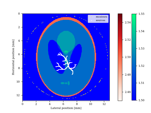
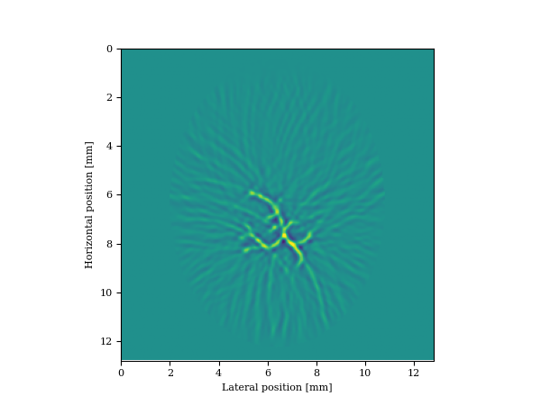
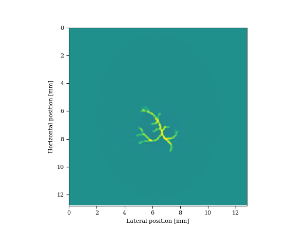
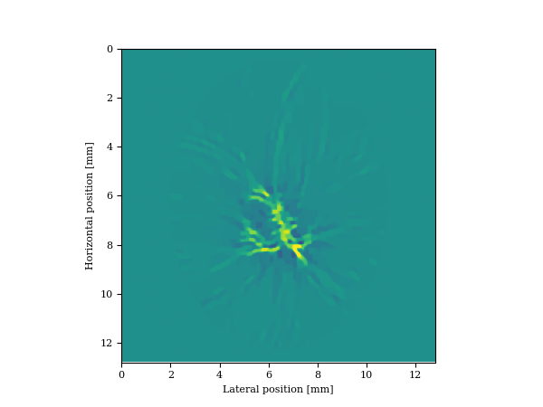
Perhaps the most straightforward application of Equation \(\ref{eq:opto}\) is in photoacoustic imaging where an unknown distribution of endogenous optical or thermal contrast sources, the object of interest, are stimulated by laser beams or radio waves. In most applications of this imaging modality, the constant or smoothly varying acoustic velocity model is assumed to be known and the “exploding reflector” induced by the laser pulse is the unknown. While good results via back propagation of the observed wavefields are possible, these results typically rely on high fidelity data collected at high spatial sampling rates (B. T. Cox et al., 2007), which puts pressure on the acquisition system where large numbers of channels come at a premium. We show that by adding a hand-crafted constraint (total-variation norm in this case, see also C. Zhang et al. (2014); Sharan et al. (2018)) to Equation \(\ref{eq:opto}\), we can remove subsampling related artifacts by solving for a given smooth background velocity model \(\mathbf{m}_0\) \[ \begin{equation} \min_{\mathbf{u}}\frac{1}{\sigma^2}\|\mathbf{d}-{F}[\mathbf{m}]\ast_t\mathbf{{q}}^e[\mathbf{u}]\|_2^2\quad\text{s.t.}\quad \|\mathbf{u}\|_{TV}\leq \tau. \label{eq:opto-constrained} \end{equation} \] In this equation, we added the total-variation norm as a handcrafted constraint using the approach of Peters et al. (2018). To evaluate the performance of this approach, we consider a thermoacoustic imaging example of a miniaturized Shepp Logan phantom, which we converted to acoustic wavespeeds (Clement, 2013). This imaging problem that operated at \(5\,\mathrm{MHz}\) is challenging because of the skull, which has a high velocity of \(2.5\,\mathrm{km/s}\). Assuming that radio waves can penetrate the skull, a thermoacoustic response can be triggered emanating from the white-color blood vessels (see Figure 1a). To further complicate things, we fivefold randomly subsampled the receivers and compare the reconstruction via back propagation with solving Equation \(\ref{eq:opto-constrained}\). Data is generated in the true velocity model while the inversion is carried out in a smoothed kinematically correct velocity model. The results are summarized in Figure 1 from which we can draw the following conclusions: (i) as predicted by compressive sensing, inversions with the TV-norm constraint are robust w.r.t. randomized receiver subsampling compared to imaging via back propagation (cf. Figures 1b & 1c) and (ii) carrying out the imaging in a spatially varying velocity model (not constant water speed) is essential in order to image through the skull (cf. Figures 1c & 1d).

Case II — Seismic imaging w/ extended sources

Even though Equation \(\ref{eq:opto}\) seems outside the realm of regular exploration seismology, there is a direct relation between this equation and recently proposed extensions of FWI designed to mitigate the effects of cycle skipping—i.e., the existence of parasitic local minima. To mitigate the possible adverse effects of these local minima, several “explain away” approaches have been proposed where additional slack/latent variables are introduced that give the problem more freedom to fit observed data even though the starting model for the velocities is wrong. Without these extra variables, the gradient has a tendency to point in the wrong direction sending FWI on a road of failure.

Extended formulations, on the other hand, may overcome this problem, in certain situations, by fitting the data, by minimizing over the slack variable first, followed by computing the gradient of the reduced objective as described above (cf. Equations \(\ref{eq:opto}\) and \(\ref{eq:reduced-opto}\)). Examples of this type of approach include Adaptive Waveform Inversion (AWI, Warner and Guasch, 2016), where trace-by-trace Wiener filters are introduced that match the observed and simulated traces, followed by a model update designed to turn these filters into zero-phase spikes; Wavefield Reconstruction Inversion (WRI, van Leeuwen and Herrmann, 2013, 2015), where a data-augmented wave equation is solved that matches the physics as well as the observed data, followed by taking a gradient step that updates the velocity model such that the wave equation itself holds (i.e., by focusing the augmented wavefield onto the sources); and extended waveform inversion with volumetric sources (Huang et al., 2018), where source extensions are used to match the observed data, followed by computing the gradient of the reduced objective. Equation \(\ref{eq:opto}\) is an instance of this latest approach where a source focusing penalty term is added as regularization. In this case we have, \(R(\mathbf{u})=\|\mathbf{W}\mathbf{u}\|_2^2\) where \(\mathbf{W}\) is an annihilator constructed in such a way that the extended source is in its null space when focussed—i.e., \(R(\delta(\mathbf{x}-\mathbf{x}_s))=0\). This can be achieved by setting \(\mathbf{W}\mathbf{u}=|\mathbf{x}-\mathbf{x}_s|\mathbf{u}\) (Huang et al., 2018).

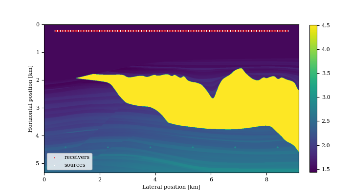
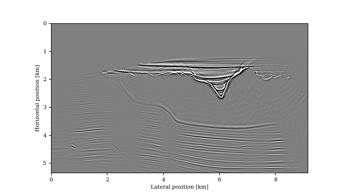
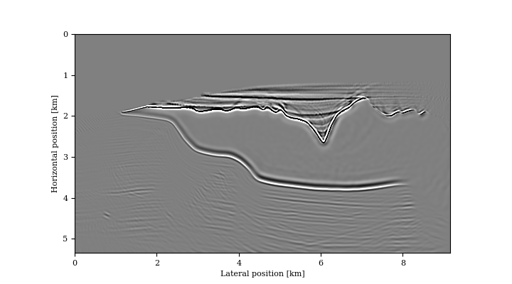
While the above approach has been used successfully to mitigate some of the effects of local minima in FWI, we show that this approach can also be used to migrate by solving for \(\mathbf{\bar{u}}\) first, by running LSQR on Equation \(\ref{eq:opto}\), followed by computing the gradient of the reduced objective with the inverse-scattering imaging condition (P. A. Witte et al., 2019b), which is designed to reduce tomographic artifacts. As we can see in Figure 2, this approach is indeed capable of producing high-fidelity images in complex models without the need to know the exact location and the directivity pattern of the sources. The interesting aspect of this two-stage approach is that we can image as long as we know the firing times of the different source experiments, which opens a new perspective on medical imaging.

Case III — Photoextended imaging

Contrary to seismic imaging, the field of medical imaging comprises of a wide range of different imaging modalities where different external stimuli are used to create an image with induced ultrasonic waves. Photoacoustic imaging is a good example of such an approach where laser light induces ultrasonic contrast sources, which can be imaged as we described under Case I. However, we can take this imaging modality a step further by using the methodology described under Case II. Contrary to conventional photoacoustic imaging, we use these contrasts as “active” sources insonifying the specimen as a whole.

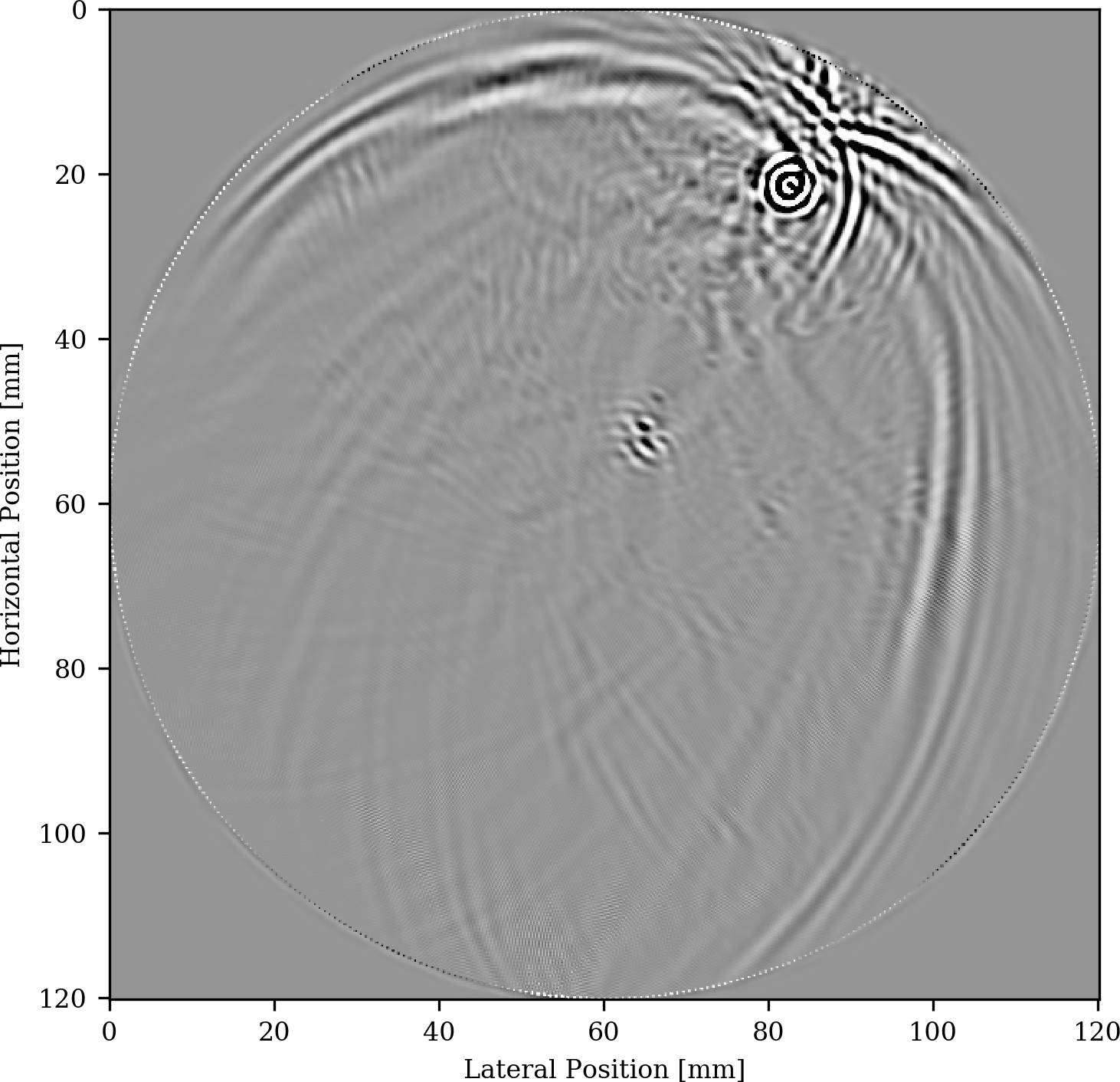
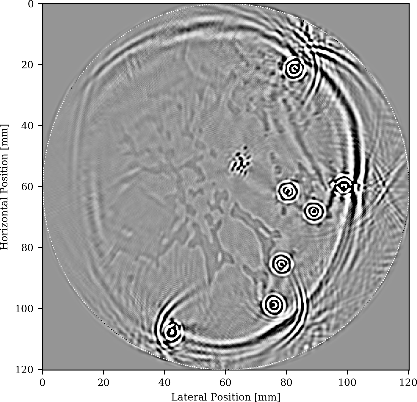
For this purpose, let us consider a 2D example of breast imaging where we are interested in finding microcalcifications (calcium oxalate) that could be indicative of breast cancer. To create an image, we assume that we are able to carry out independent photo-source experiments where ultrasonic “point sources” are triggered with laser light. We assume that these sources are located in blood vessels. We repeat this multiple times. Since we do not know where the blood vessels are, we do not apply focussing but instead we solve for each source separately using \(5\) iterations of LSQR, followed by computing the gradients, as in Equation \(\ref{eq:gradient-opto}\), which we stack into a single image. The setup for our experiment is depicted in Figure 3a and includes \(7\) different opto-induced sources placed in blood vessels and denoted by the white crosses and densely sampled receivers placed in a circular fashion around the breast. As we can see from Figure 3c, we obtain a clear image not only of the microcalcifications but also of the fat and fibroglandular tissue.

Observations

We believe that these experiments demonstrate that imaging algorithms originally motivated by specific challenges encountered in seismic problems can be applied in some interesting medical imaging scenarios. We make this assertion under the assumption that we are in the correct physical regime and that we have access to adequate computational resources. If this is indeed the case, there are exciting possibilities because wave-equation based inversion, in tandem with regularization with contraints and deep priors, opens the way towards high-fidelity high-resolution images including uncertainty quantification.

Related materials

In order to facilitate the reproducibility of the results herein discussed, a Julia implementation of this work is made available on the SLIM GitHub page https://github.com/slimgroup/Software.SEG2020.

Acknowledgements

Felix J. Herrmann would like to thank the Georgia Institute of Technology and the Georgia Research Alliance for their financial support.