Learned imaging with constraints and uncertainty quantification

The seismic imaging problem

In least-squares imaging, we are interested in inverting the following inconsistent ill-conditioned linear inverse problem: \[ \begin{equation} \minim_x \frac{1}{2}\sum_{i=1}^N\|y_i-A_ix\|_2^2. \label{eq:LSQR} \end{equation} \] In this expression, the unknown vector \(x\) represents the image, \(y_i,\, i=1, \ldots, N\) the observed data from \(N\) source experiments and \(A_i\) the discretized linearized forward operator for the \(i\text{th}\) source experiment. Despite being overdetermined, the above least-squares imaging problem is challenging. The linear systems \(A_i\) are large, expensive to evaluate, and inconsistent because of noise and/or linearization errors.

As in many inverse problems, solutions of problem \(\ref{eq:LSQR}\) benefit from adding prior information in the form of penalties or preferentially in the form of constraints, yielding \[ \begin{equation} \minim_x \frac{1}{2}\sum_{i=1}^N\|y_i-A_ix\|_2^2 \quad\text{subject to}\quad x\in\mathcal{C} \label{eq:constrained-LSQR} \end{equation} \] with \(\mathcal{C}\) representing a single or multiple (convex) constraint set(s). This approach offers the flexibility to include multiple handcrafted constraints. Several key issues remain, namely; (i) we can not afford to work with all \(N\) experiments when computing gradients for the above data-misfit objective; (ii) constrained optimization problems converge slowly; (iii) handcrafted priors may not capture complexities of natural images; (iv) it is non-trivial to obtain uncertainty quantification information.

Stochastic linearized Bregman

To meet the computational challenges that come with solving problem \(\ref{eq:constrained-LSQR}\) for non-differentiable structure promoting constraints, such as the \(\ell_1\)-norm, we solve problem \(\ref{eq:constrained-LSQR}\) with Bregman iterations for a batch size of one. The \(k\text{th}\) iteration reads \[ \begin{equation} \begin{aligned} \begin{array}{lcl} \tilde{x} & \leftarrow & \tilde{x}-t_k A_k^\top(A_kx-y_k)\\ x & \leftarrow & \mathcal{P}_{\mathcal{C}} (\tilde{x}) \end{array} \end{aligned} \label{eq:bregman-iterations} \end{equation} \] with \(A_k^\top\) the adjoint of \(A_k\) , where \(A_k \in \left \{ A_i \right \}_{i=1}^{N}\), and \[ \begin{equation} \mathcal{P}_{\mathcal{C}} (\tilde{x}) = \argmin_{x} \frac{1}{2} \| x - \tilde{x} \|_2^2 \quad \text{subject to} \quad x \in \mathcal{C} \label{proj_card} \end{equation} \] being the projection onto the (convex) set and \(t_k={\|A_kx-y_k\|_2^2}/{\|A_k^\top(A_kx-y_k)\|_2^2}\) the dynamic steplength. Contrary to the Iterative Shrinkage Thresholding Algorithm (ISTA), we iterate on the dual variable \(\tilde{x}\). Moreover, to handle more general situations and to ensure we are for every iteration feasible (= in the constraint set) we replace sparsity-promoting thresholding with projections that ensure that each model iterate remains in the constraint set. As reported in Witte et al. (2019), iterations \(\ref{eq:bregman-iterations}\) are known to converge fast for pairs \(\{y_k,\,A_k\}\) that are randomly drawn, with replacement, from iteration to iteration. As such, Equation \(\ref{eq:bregman-iterations}\) can be interpreted as stochastic gradient descent on the dual variable.

Deep prior with constraints

Handcrafted priors, encoded in the constraint set \(\mathcal{C}\), in combination with stochastic optimization, where we randomly draw a different source experiment for each iteration of Equation \(\ref{eq:bregman-iterations}\), allow us to create high-fidelity images by only working with random subsets of the data. While encouraging, this approach relies on handcrafted priors encoded in the constraint set \(\mathcal{C}\). Motivated by recent successes in machine learning and deep convolutional networks (CNNs) in particular, we follow Van Veen et al. (2018), Dittmer et al. (2018) and Y. Wu and McMechan (2019) and propose to incorporate CNNs as deep priors on the model. Compared to handcrafted priors, deep priors defined by CNNs are less biased since they only require the model to be in the range of the CNN, which includes natural images and excludes images with unnatural noise. In its most basic form, this involves solving problems of the following type (Van Veen et al. 2018): \[ \begin{equation} \minim_w \frac{1}{2}\|y-Ag(z,w)\|_2^2. \label{eq:deep-prior} \end{equation} \] In this expression, \(g(z,w)\) is a deep CNN parameterized by unknown weights \(w\) and \(z\sim\mathrm{N}(0,1)\) is a fixed random vector in the latent space. In this formulation, we replaced the unknown model by a neural net. This makes this formulation suitable for situations where we do not have access to data-image training pairs but where we are looking for natural images that are in the range of the CNN. In recent work by Van Veen et al. (2018), it is shown that solving problem \(\ref{eq:deep-prior}\) can lead to good estimates for \(x\) via the CNN \(g(z,\widehat{w})\) where \(\widehat{w}\) is the minimizer of problem \(\ref{eq:deep-prior}\) highly suitable for situations where we only have access to data. In this approach, the parameterization of the network by \(w\) for a fixed \(z\) plays the role of a non-linear redundant transform.

While using neural nets as strong constraints may offer certain advantages, there are no guarantees that the model iterates remain physically feasible, which is a prerequisite if we want to solve non-linear imaging problems that include physical parameters (Esser et al. 2018; Peters, Smithyman, and Herrmann 2018). Unless we pre-train the network, early iterations while solving problem \(\ref{eq:deep-prior}\) will be unfeasible. Moreover, as mentioned by Van Veen et al. (2018), results from solving inverse problems with deep priors may benefit from additional types of regularization. We accomplish this by combining hard handcrafted constraints with a weak constraint for the deep prior resulting in a reformulation of the problem \(\ref{eq:deep-prior}\) into \[ \begin{equation} \minim_{x\in \mathcal{C},\,w} \frac{1}{2}\|y-Ax\|_2^2 + \frac{\lambda^2}{2}\|x-g(z,w)\|_2^2. \label{eq:constrained-deep-prior} \end{equation} \] In this expression, the deep prior appears as a penalty term weighted by the trade-off parameter \(\lambda>0\). In this weak formulation, \(x\) is a slack variable, which by virtue of the hard constraint will be feasible throughout the iterations.

The above formulation offers flexibility to impose constraints on the model that can be relaxed during the iterations as the network is gradually “trained”. We can do this by either relaxing the constraint set (eg. by increasing the size of the TV-norm ball) or by increasing the trade-off parameter \(\lambda\).

Learned imaging via expectation maximization

So far, we used the neural network to regularize inverse problems deterministically by selecting a single latent variable \(z\) and optimizing over the network weights initialized by white noise. While this approach may remove bias related to handcrafted priors, it does not fully exploit documented capabilities of generative neural nets, which are capable of generating realizations from a learned distribution. Herein lies both an opportunity and a challenge when inverse problems are concerned where the objects of interest are generally not known a priori. Basically, this leaves us with two options. Either we assume to have access to an oracle, which in reality means that we have a training set of images obtained from some (expensive) often unknown imaging procedure, or we make necessary assumptions on the statistics of real images. In both cases, the learned priors and inferred posteriors will be biased by our (limited) understanding of the inversion process, including its regularization, or by our (limited) understanding of statistical properties of the unknown e.g. geostatistics (Mosser, Dubrule, and Blunt 2018). The latter may lead to perhaps unreasonable simplifications of the geology while the former may suffer from remnant imprint of the nullspace of the forward operator and/or poor choices for the handcrafted and deep priors.

Training phase

Contrary to approaches that have appeared in the literature, where the authors assume to have access to a geological oracle (Mosser, Dubrule, and Blunt 2018) to train a GAN as a prior, we opt to learn the posterior through inversion deriving from the above combination of hard handcrafted constraints and weak deep priors with the purpose to train a network to generate realizations from the posterior. Our approach is motivated by Han et al. (2017) who use the Expectation Maximization (EM) technique to train a generative model on sample images. We propose to do the same but now for seismic data collected from one and the same Earth model.

To arrive at this formulation, we consider each of the \(N\) source experiments with data \(y_k\) as separate datasets from which images \(x_k\) can in principle be inverted. In other words, contrary to problem \(\ref{eq:LSQR}\), we make no assumptions that the \(y_k\) come from one and the same \(x\) but rather we consider \(n\ll N\) different batches each with their own \(x_k\). Using the these \(y_k\), we solve an unsupervised training problem during which

• \(n\) minibatches of observed data, latent, and slack variables are paired into tuples \(\{y_i,x_i,z_i\}_{i=1}^n\) with the latent variables \(z_i\)’s initialized as zero-centered white Gaussian noise, \(z_i\sim N(0,I)\). The slack variables \(x_i\)’s are computed by the numerically expensive Bregman iterations, which during each iteration work on the randomized source experiment of each minibatch.

• latent variables \(z_i\)’s are sampled from \(p(z_i | x_i, w)\) by running \(l\) iterations of Stochastic Gradient Langevin Dynamics (SGLD, Welling and Teh (2011)) (Equation \(\ref{eq:Langevin}\)), where \(w\) is the current estimate of network weights, and \(x_i\)’s are computed with Bregman iterations (Equation \(\ref{eq:constrained-bregman-iteration}\)). These iterations for the latent variables are warm-started while keeping the network weights \(w\) fixed. This corresponds to an unsupervised inference step where training pairs \(\{x_i,z_i\}_{i=1}^n\) are created. Uncertainly in the \(z_i\)’s is accounted for by SGLD iterations (Han et al. 2017; Mosser, Dubrule, and Blunt 2018).

• the network weights are updated using \(\{x_i,z_i\}_{i=1}^n\) with a supervised learning procedure. During this learning step, the network weights are updated by sample averaging the gradients w.r.t. \(w\) for all \(z_i\)’s. As stated by Han et al. (2017), we actually compute a Monte Carlo average from these samples.

By following this semi-supervised learning procedure, we expose the generative model to uncertainties in the latent variables by drawing samples from the posterior via Langevin dynamics that involve the following iterations for the pairs \(\{x_i,\, z_i\}_{i=1}^n\) \[ \begin{equation} z_i\leftarrow z_i-\frac{\varepsilon}{2}\nabla_z\left ( \lambda^2 \|x_i - g(z_i,w))\|_2^2 + \left \| z_i \right \|_2^2 \right ) +\mathcal{N}(0, \varepsilon I) \label{eq:Langevin} \end{equation} \] with \(\varepsilon\) the steplength. Compared to ordinary gradient descent, \(\ref{eq:Langevin}\) contains an additional noise term that under certain conditions allows us to sample from the posterior distribution, \(p(z_i | x_i, w)\). The training samples \(x_i\) came from the following Bregman iterations in the outer loop \[ \begin{equation} \begin{aligned} \begin{array}{lcl} \tilde{x}_i & \leftarrow & \tilde{x}_i- t_k \left ( A_k^\top(A_kx_i-y_k) + \lambda^2 (x_i-g(z_i,w)) \right)\\ x_i & \leftarrow & \mathcal{P}_{\mathcal{C}} (\tilde{x}_i). \end{array} \end{aligned} \label{eq:constrained-bregman-iteration} \end{equation} \] After sampling the latent variables, we update the network weights via for the \(z_i\)’s fixed \[ \begin{equation} w \leftarrow w -\eta \nabla_w \sum_{i=1}^n\|x_i-g(z_i,w)\|_2^2 \label{eq:constrained-bregman-iterations-b} \end{equation} \] with \(\eta\) steplength for network weights.

Conceptually, the above training procedure corresponds to carrying out \(n\) different inversions for each data set \(y_i\) separately. We train the weights of the network as we converge to the different solutions of the Bregman iterations for each dataset. As during Elastic-Averaging Stochastic Gradient Descent (Zhang, Choromanska, and LeCun 2015,Chaudhari et al. (2016)), \(x_i\)’s have room to deviate from each other when \(\lambda\) is not too large. Our approach differs in the sense that we replaced the center variable by a generative network.

Example

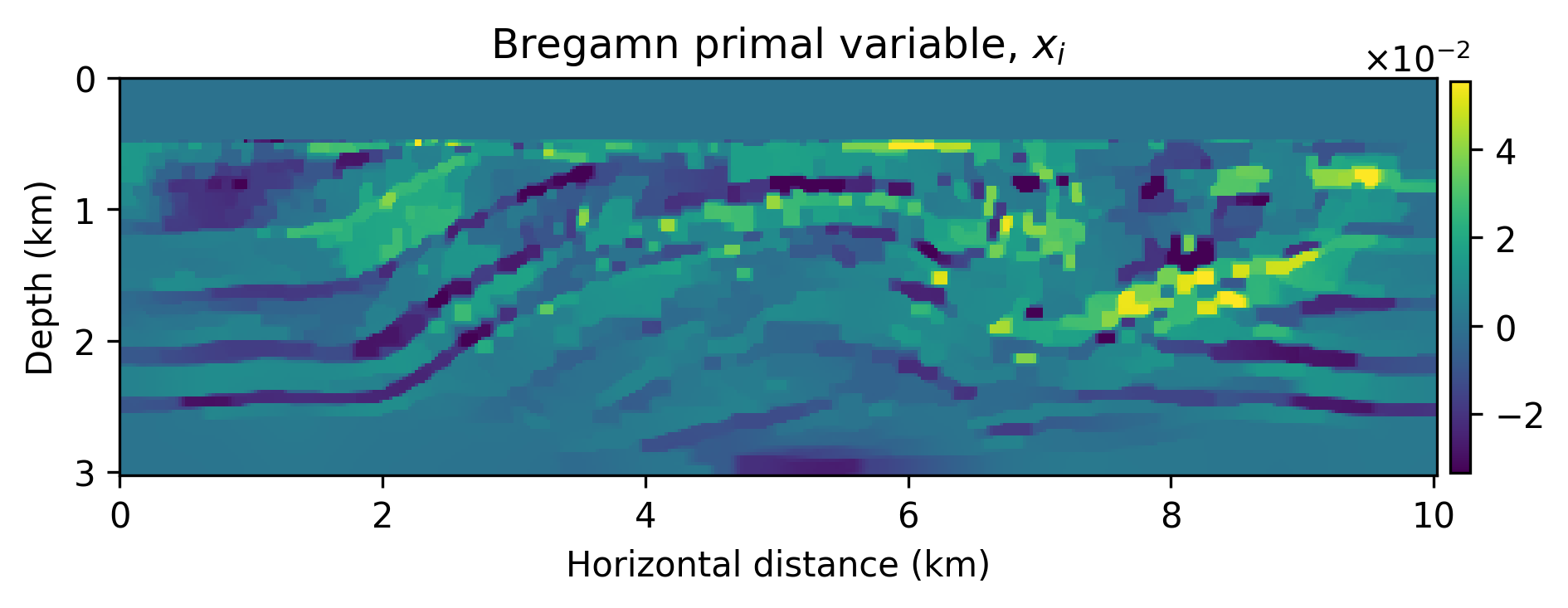
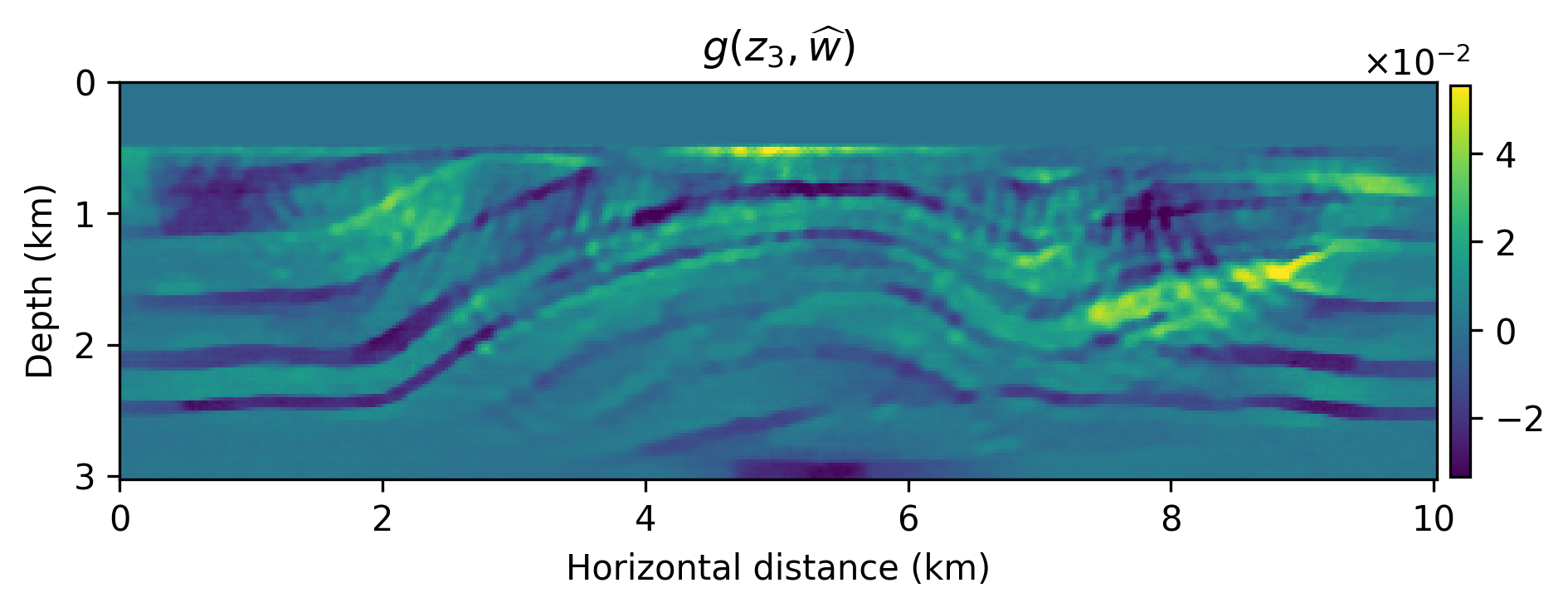
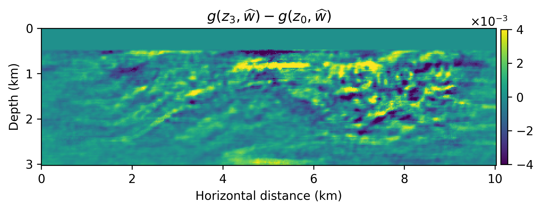
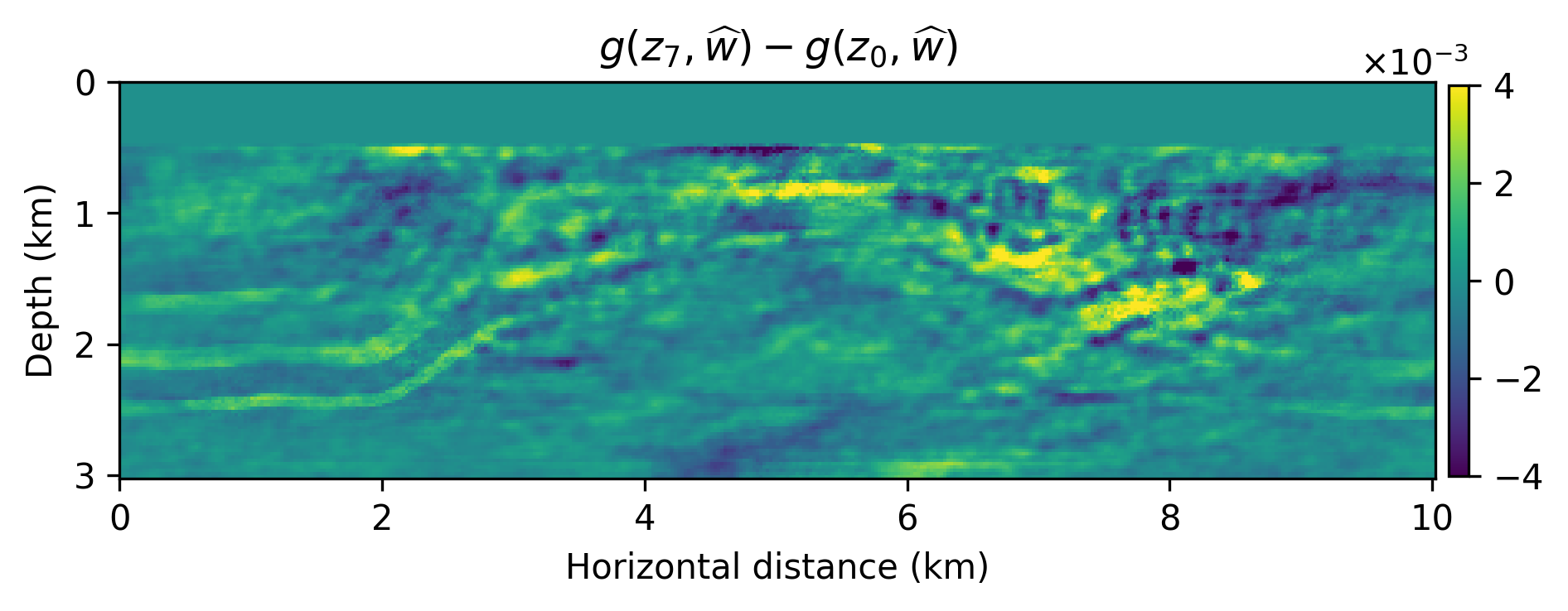
We numerically conduct a survey where the source experiments contain severe incoherent noise and coherent linearization errors: \(e=(F_k(m+\delta m)-F_k(m)-\nabla F_k(m)\delta m)\), where \(A_k=\nabla F_k\) is the Jacobian and \(F_k(m)\) is the nonlinear forward operator with \(m\) the known smooth background model and \(\delta m\) the unknown perturbation (image). The signal-to-noise ratio of the observed data is \(-11.37\) dB. The results of this experiment are included in Figure 1 from which we make the following observations. First, as expected the models generated from \(g(z,\widehat{w})\) are smoother than the primal Bregman variable. Second, there are clearly variations amongst the different \(g(z,\widehat{w})\)’s and these variations average out in the mean, which has fewer imaging artifacts.

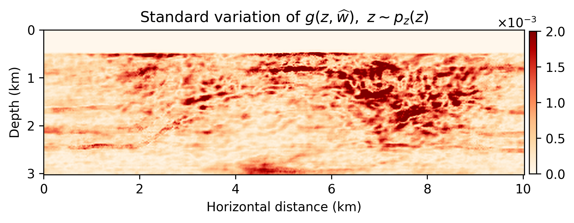
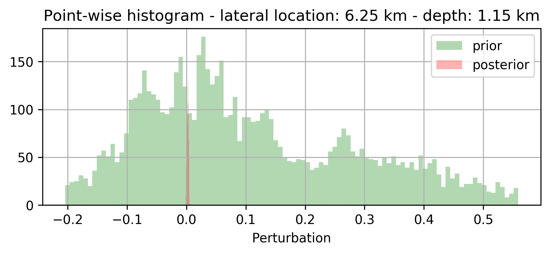
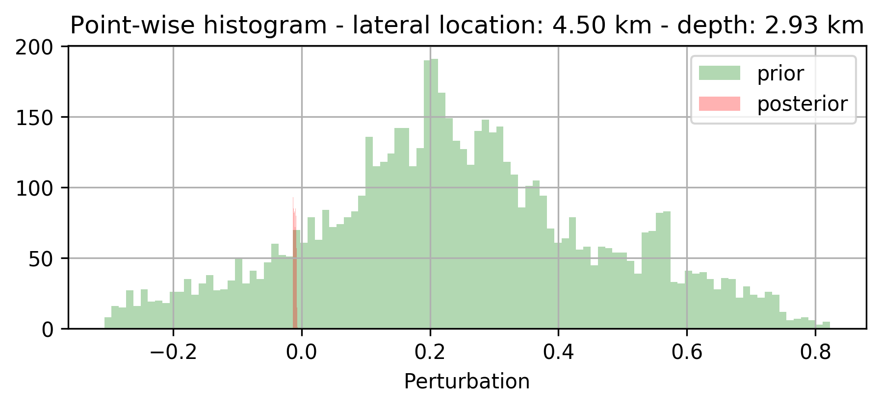
Because we were able to train the \(g(z,w)\) as a “byproduct” of the inversion, we are able to compute statistical information from the trained generative model that may give us information about the “uncertainty”. In Figure 2, we included a plot of the pointwise standard deviation , computed with \(3200\) random realizations of \(g(z, w), \ z\sim p_z(z)\), and two examples of sample “prior” (before training) and “posterior” distribution. As expected, the pointwise standard deviations shows a reasonable sharpening of the probabilities before and after training through inversion. We also argue that the areas of high pointwise standard deviation coincide with regions that are difficult to image because of the linearization error and noise.

Discussion and Conclusions

In this work, we tested an inverse problem framework which includes hard constraints and deep priors. Hard constraints are necessary in many problems, such as seismic imaging, where the unknowns must belong to a feasible set in order to ensure the numerical stability of the forward problem. Deep priors, enforced through adherence to the range of a neural network, provide an additional, implicit type of regularization, as demonstrated by recent work (Van Veen et al. 2018,Dittmer et al. (2018)), and corroborated by our numerical results. The resulting algorithm can be mathematically interpreted in light of expectation maximization methods. Furthermore, connections to elastic averaging SGD (Zhang, Choromanska, and LeCun 2015) highlight potential computational benefits of a parallel (synchronous or asynchronous) implementation.

On a speculative note, we argue that the presented method, which combines stochastic optimization on the dual variable with on-the-fly estimation of the generative model’s weights using Langevin dynamics, reaps information on the “posterior” distribution leveraging multiplicity in the data and the fact that the data is acquired over one and the same Earth model. Our preliminary results seem consistent with a behavior to be expected from a “posterior” distribution.