Random sampling: new insights into the reconstruction of coarsely-sampled wavefields

Reconstruction by denoising

Consider the following linear forward model for the interpolation problem

$$\mathbf{y} = \tensor{R}\mathbf{f}_0,$$ (2)

where $\mathbf{y}\in\mathbb{R}^n$ represents the data acquired at sub-Nyquist rate, $\mathbf{f}_0\in\mathbb{R}^N$ the densely-sampled data to be recovered, and $\tensor{R}\in\mathbb{R}^{n\times N}$ the restriction operator that selects the acquired samples among the desired samples. Assume $\mathbf{f}_0$ has a sparse representation $\mathbf{x}_0$ in some transform domain $\tensor{S}$ where random sampling creates incoherent noise (e.g. Fourier domain, $\tensor{S}:=\tensor{F}$ ), then interpolation to a dense grid becomes a denoising problem in the $\tensor{S}$ domain (Donoho et al., 2007). This problem is solved by the following nonlinear sparsity-promoting optimization (Hennenfent and Herrmann, 2006; Candes et al., 2005)

$$\tilde{\mathbf{x}} = \arg\min_{\mathbf{x}}\vert\vert\mathbf{x}\vert\vert _1 \quad\mathbf{y}=\tensor{RS}^H\mathbf{x},$$ (3)

where the symbol $\tilde{\mbox{}}$ represents an estimated quantity, and   $^H$ the conjugate tranpose. The interpolated result is given by $\tilde{\mathbf{f}}=\tensor{S}^H\tilde{\mathbf{x}}$ . Note that, if the sampling at sub-Nyquist rate creates coherent noise in the $\tensor{S}$ domain (see e.g. Fig. 1(b) when $\tensor{S}:=\tensor{F}$ ), the separation between signal and noise generated by the acquisition in the $\tensor{S}$ domain is much more delicate (if not impossible) just by imposing a sparsity constraint. We illustrate this comment by a simple 1-D experiment.
We define $\tensor{S}$ as the discrete cosine transform. We generate a vector $\mathbf{x}_0$ of length $N=600$ containing $k$ nonzero entries with random amplitudes, random signs, and random positions and construct $\mathbf{f}_0=\tensor{S}^H\mathbf{x}_0$ . The observations $\mathbf{y}$ are obtained by down-sampling $\mathbf{f}_0$ either regularly or randomly by a factor of $2,\ldots ,6$ . Finally, we solve Eq. 3 and compare the estimated representation $\tilde{\mathbf{x}}$ of $\mathbf{f}_0$ to its true representation $\mathbf{x}_0$ . The reconstruction error is measured as the number of false detections in the discrete cosine transform domain. The results presented in Fig. 2 are averaged over 50 independent experiments. Figs. 2(a) and 2(b) show the recovery curves for regular and random downsampling, respectively. Each curve represents the results obtained for a given subsampling factor. Fig. 2(a) shows that, regardless of the subsampling factor and the sparsity of $\mathbf{f}_0$ in the discrete cosine transform domain, the solution of Eq. 3 is corrupted by some noise. However, Fig. 2(b) shows that there is a sparsity zone for each subsampling factor such that the reconstruction is perfect, i.e. no false detection. The smaller the subsampling factor, the wider the perfect reconstruction zone.

phasediagREG,phasediagIRREG
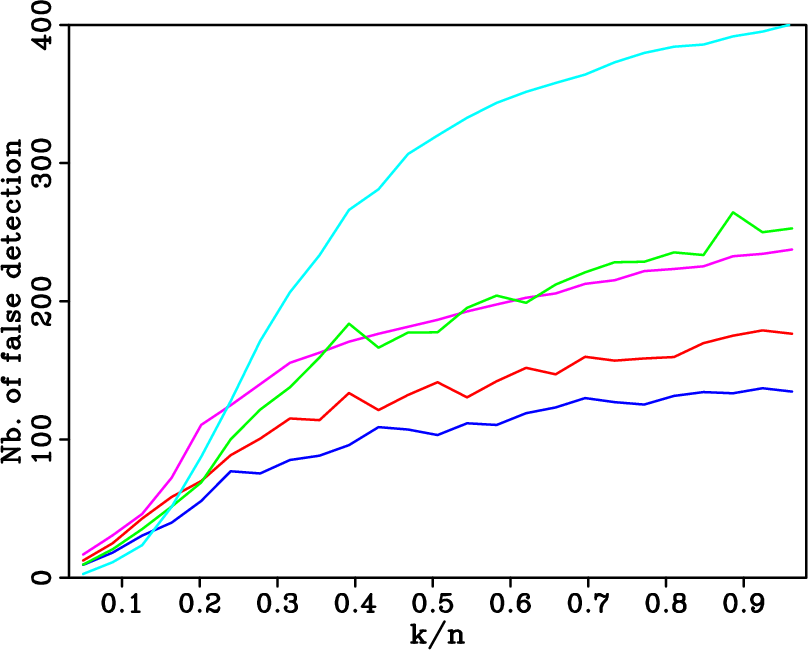
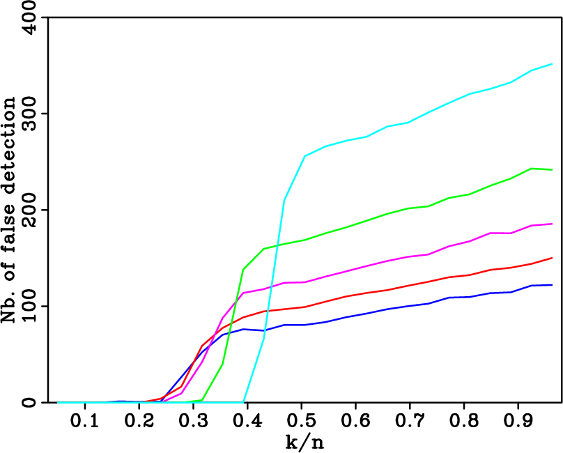
Figure 2. Average recovery curves from sub-Nyquist rate samplings using nonlinear sparsity-promoting optimization. Average recovery curves (a) from regular sub-samplings by $2,\ldots ,6$ curves and (b) from random sub-samplings by the same factors as in (a)

Random sampling: new insights into the reconstruction of coarsely-sampled wavefields