![]()
![]()
Summary
By building on recent advances in the use of randomized trace estimation to drastically reduce the memory footprint of adjoint-state methods, we present and validate an imaging approach that can be executed exclusively on accelerators. Results obtained on field-realistic synthetic datasets, which include salt and anisotropy, show that the method produces high-fidelity imaging results. These findings open the enticing perspective of 3D wave-based inversion technology with a memory footprint that matches the hardware and that runs exclusively on clusters of GPUs without the undesirable need to offload certain tasks to CPUs.
Introduction
Subsurface imaging has recently thrived building on advances in wave-equation based methods such as Full-Waveform Inversion (FWI) and Reverse-Time Migration (RTM) (Tarantola, 1984, Virieux and Operto (2009)). However, these methods rely on extremely high computational and memory costs, which explains the relative limited widespread adaptation of these technologies. Unfortunately, exceedingly large memory footprints are inherent to the adjoint-state method (Lions, 1971, Tarantola (1984)), which requires storage (in memory, on disk, possibly compressed) of the complete time history of the forward modeled wavefield in order to compute the imaging condition that correlates this forward wavefield with the time-reversed solution of the adjoint wave equation. Because saving forward modeled wavefields requires terabytes of memory for industry scale high-frequency 3D imaging, memory usage has been and continues to be a major bottleneck on standard with the exception perhaps of dedicated high-memory nodes available in the cloud. While dedicated nodes relief some of the memory pressure, they do not allow use of accelerators to speed up computations. Contrary to conventional computer hardware, memory on accelerators comes at a premium, which is problematic given the large memory footprint of adjoint-state methods. To address this problem, several methods have been proposed over the years where excessive memory footprints are offset by incurring computational overhead. A good example of such an approach is the method of optimal checkpointing proposed by Griewank and Walther (2000) and Symes (2007). This method was initially introduced to tackle memory limitation of CPUs and has been used successfully in 3D seismic applications. To further limit the computational overhead, N. Kukreja et al. (2020) recently supplemented this approach by adding on-the-fly compression and decompression of the forward wavefields. In situations where the wave physics is reversible, researchers (McMechan, 1983, Mittet (1994), Raknes and Weibull (2016)) have shown that forward wavefields can also be recomputed from boundary values. Unfortunately, both approaches are challenged by underlying assumptions. They also require a relative high of algorithmic complexity. This explains why GPUS-native implementations of adjoint-state methods including on-the-fly compression remain illusive.
While recomputing forward wavefields as part of memory-footprint mitigation certainly has its merits, there exist simpler randomized approaches where memory use is traded against computational overhead and controllable error. Unlike approaches that aim to compute gradients exactly, these methods approximate the gradient with the aim to reduced computational and memory costs at the expense of a controllable loss in accuracy. Examples of such an approach include to working with random subsets of shots (Friedlander and Schmidt, 2012) or simultaneous shots (Romero et al., 2000, Krebs et al. (2009b), Moghaddam et al. (2013), Haber et al. (2015), Leeuwen and Herrmann (2013)), or with randomized singular value decompositions (Leeuwen et al., 2017, Yang et al. (2021)) and random-trace estimation. The latter was used by Haber et al. (2015) to analyze computational speedups of full-waveform with computational simultaneous sources. As long as the errors are controlled, these methods lead to equivalent inversion results at fraction of the computational costs (e.g. speedups of a factors of seven have been reported for FWI (Krebs et al., 2009a)). Following ideas from randomized linear algebra to estimate the trace of a matrix, M. Louboutin and Herrmann (2021) proposed an approximation of the adjoint-state method that leads to major memory improvements and is relatively easy to implement and supported by theory (Avron and Toledo, 2011, Meyer et al. (2020)), guaranting convergence including bounds on the accuracy. However, unlike other approximate methods, such as on-the-fly Fourier-based (P. A. Witte et al., 2019b) or lossy compression-based algorithms(N. Kukreja et al., 2020), the artifacts introduced by the proposed randomized trace estimation are incoherent and appear as Gaussian-like noise, which can be handled easily by sparsity-promoting imaging (P. A. Witte et al., 2019b). While the initial results of the randomized trace estimation on a simple 2D synthetic were encouraging (M. Louboutin and Herrmann, 2021), we submit the proposed approximation to additional scrutiny by considering complex imaging examples that involve salt (SEAM model (Fehler and Keliher, 2011)) and anisotropy (Thomsen, 1986) (BP TTI model).
Our contributions are organized as follows. First, we briefly introduce randomized trace estimation and its computational benefits during RTM and the formation of horizontal subsurface-offset image volumes (W. W. Symes, 2008). Next, we show its application to two representative examples, long-offset subsalt imaging on the 2D SEAM acoustic model with a sparse ocean-bottom node acquisition, and TTI anisotropic imaging of the 2D BP TTI model. With these examples, we validate the computational efficiency and practicality of our method on GPUs available on Azure (the Standard_NC6 virtual machine).
Methodology
Before we demonstrate the advocacy of the proposed methodology on complex imaging problems, let us first quickly discuss how randomized trace estimation can be used to reduce the memory footprint of adjoint-state wave-based seismic imaging. We do this by showing that applying the imaging condition corresponds to computing the trace of a matrix.
Randomized trace estimation
Approximating (Avron, Meyer et al., 2020) the identity \(\mathbf{I}\) by
\[
\begin{equation}
\operatorname{tr}(\mathbf{A}) =\operatorname{tr}\left(\mathbf{A} \mathbb{E}\left[\mathbf{z} \mathbf{z}^{\top}\right]\right) =\mathbb{E}\left[\operatorname{tr}\left(\mathbf{A} \mathbf{z} \mathbf{z}^{\top}\right)\right]
= \mathbb{E}\left[\mathbf{z}^{\top} \mathbf{A} \mathbf{z}\right] \approx \frac{1}{r}\sum_{i=1}^r\left[\mathbf{z}^{\top}_i \mathbf{A} \mathbf{z}_i\right]= \frac{1}{r}\operatorname{tr}\left(\mathbf{Z}^\top \mathbf{A}\mathbf{Z}\right)
\label{randomtrace}
\end{equation}
\]
lies at the heart of randomized trace estimation where the \(\mathbf{z}_i\)’s are random probing vectors for which \(\mathbb{E}(\mathbf{z}^{\top}\mathbf{z})=1\) with \(\mathbb{E}\) is the stochastic expectation operator. This above estimator for the trace (sum of the diagonal of the matrix \(\mathbf{A}\), \(\operatorname{tr}(A)=\sum_i \mathbf{A}_{ii}\)) is unbiased (i.e., exact in expectation) and converges to the true trace with an error that decays with \(r\) and without access to the entries of \(\mathbf{A}\). Only actions of \(\mathbf{A}\) on the probing vectors are needed and we exploit this property and the specific structure of the matrix \(\mathbf{A}\) in gradient calculations for wave-equation based inversion. Motivated by recent work (Meyer et al., 2020, Graff-Kray et al. (2017)) we also employ a partial qr factorization (Trefethen and Bau III, 1997) that approximates the range of the matrix \(\mathbf{A}\)—i.e., we approximate the trace with probing vectors \(\begin{bmatrix}\mathbf{Q},\thicksim\end{bmatrix} = \operatorname{qr}(\mathbf{A}\mathbf{Z})\) where \(\mathbf{Z}\) is a Rademacher random matrix of \(\pm 1\).
Approximate gradient calculations
While the presented randomized approach carries over to arbitrary complex wave physics, we derive our memory reduced gradient approximation for the isotropic acoustic case where the gradient for a single source \(\delta\mathbf{m}\) can be written as \[ \begin{equation} \delta\mathbf{m} = \sum_{t=1}^{n_t} \mathbf{\ddot{u}}[t] \mathbf{v}[t]. \label{iccc} \end{equation} \] In this expression, \(\mathbf{u}[t], \mathbf{v}[t]\) are the vectorized (along space) full-space forward and adjoint wavefields at time index \(t=1\cdots n_t\) with \(n_t\) the number of timesteps. The symbol \(\ddot{}\) represents second-order time derivative. To arrive at a form where randomized trace estimation can be used, we write the above zero-lag imaging condition over time as the trace of the outer product for each space index \(\mathbf{x}\) separately. By using the dot product property, \(\sum \mathbf{x}_i \mathbf{y}_i=\mathbf{x}^\top\mathbf{y}=\operatorname{tr}(\mathbf{x}\mathbf{y}^\top)\), and the approximation in Equation \(\ref{randomtrace}\), the gradient at location \(\mathrm{x}\) becomes \[ \begin{equation} \begin{split} \delta\mathbf{m}[\mathbf{x}] = \operatorname{tr}\left(\mathbf{\ddot{u}}[\cdot, \mathbf{x}]\mathbf{v}[\cdot, \mathbf{x}]^\top\right) \approx \frac{1}{r} \operatorname{tr}\left(\bar{\ddot{\mathbf{u}}}[\cdot, \mathbf{x}]\bar{\mathbf{v}}[\cdot, \mathbf{x}]^\top\right)\quad\text{with}\quad \bar{\ddot{\mathbf{u}}}=\mathbf{Q}^\top \mathbf{\ddot{u}}, \bar{\mathbf{v}}=\mathbf{Q}^\top \mathbf{v}. \\ \end{split} \label{optr} \end{equation} \] Contrary to the sum over all timesteps \(t\), the zero-offset imaging condition in Equation \(\ref{optr}\) involves storage of the compressed wavefields for only \(r\ll n_t\) timesteps. This compression not only significantly reduces the memory footprint but it also lessens the computational cost of computing imaging conditions as a function of the horizontal subsurface offset \[ \begin{equation} \delta\mathcal{M}[\mathbf{x},\mathbf{h}] \approx \frac{1}{r} \operatorname{tr}\left(\bar{\ddot{\mathbf{u}}}[\cdot, \mathbf{x}+\mathbf{h}]\bar{\mathbf{v}}[\cdot, \mathbf{x}-\mathbf{h}]^\top\right) \label{ssoffset} \end{equation} \] with \(\mathbf{h}\) the horizontal subsurface offset and \(\delta\mathcal{M}[\mathbf{h}]\) the subsurface image volume. As with computing the zero-offset imaging condition in Equation \(\ref{optr}\), the cost of computing these volumes is also reduced by a factors of \(r/n_t\). Also notice that \(\delta\mathbf{m}[\mathbf{x}]=\delta\mathcal{M}[\mathbf{x},h]\vert_{\mathbf{h}=0}\).
Figure 1 contains subsurface offset gathers for the 2007 BP TTI model discussed in more detail below. Despite the fact that we used only a limited (\(r=64\ll n_t\)) probing factors, the images gathers are properly focused around and nearly noise free thanks to the noise stacking. Each image volume is using \(81\) offsets (\(-500m:12.5m:500m\)) and is effectively using more memory that we needed to store the compressed wavefields needed to compute these volumes, highlighting how memory frugal the proposed trace estimation method realy is.
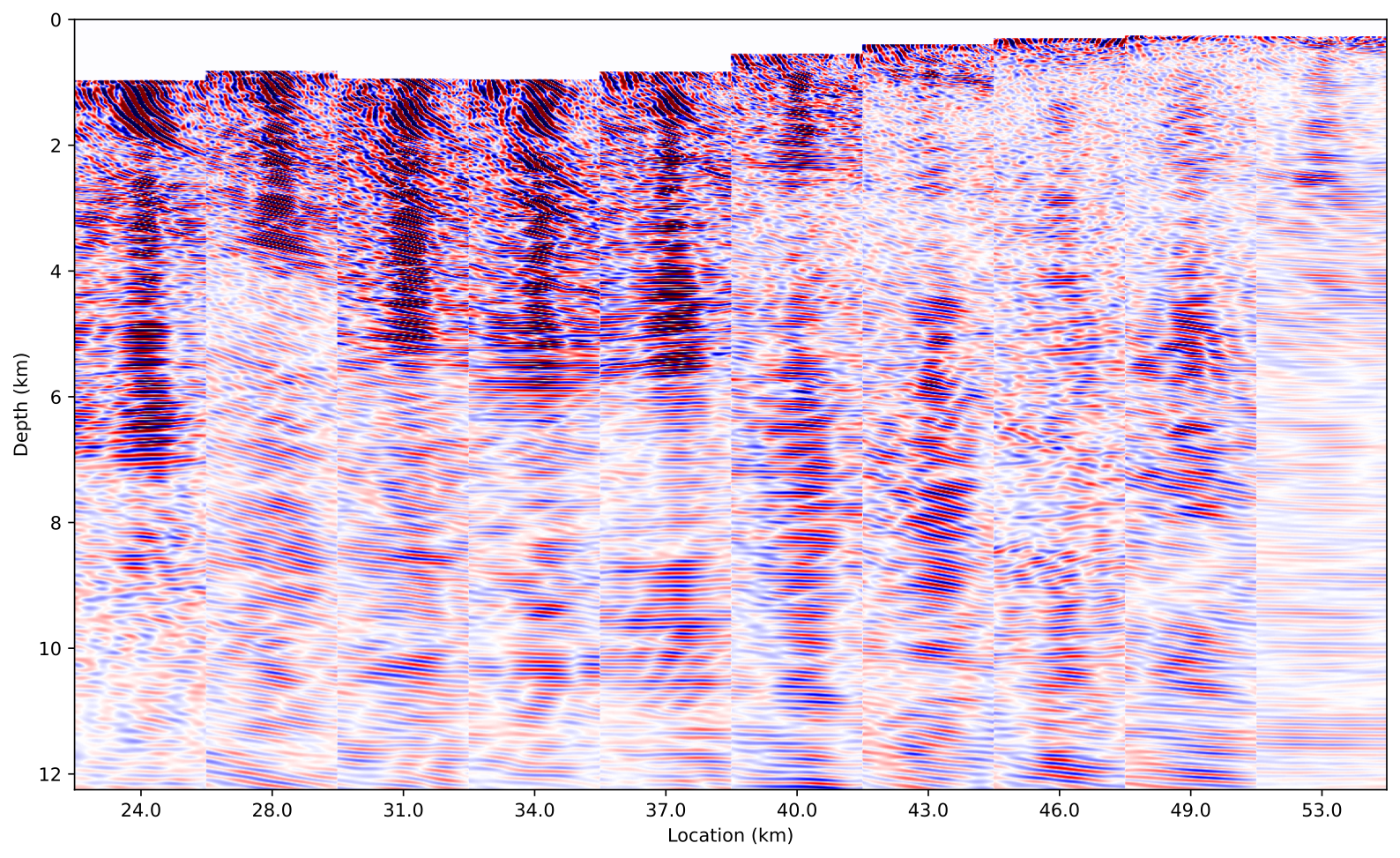
-500m to 500m horizontal offset.Synthetic case studies
To validate the proposed technology, we consider the 2D acoustic SEAM model and the 2D 2007 BP TTI model. We chose these models because they are complex and in need of a large number of timesteps. As the examples included below, we obtain reasonable RTM images for a limited number of probing vectors (\(r=64\)), yielding a memory reduction by a factor of \(100\times\)—\(150\times\) reducing the memory footprint to less than 2Gb. This drastic memory reduction allows us to fully take advantage of accelerators by performing the RTM imaging natively on GPUs without relying on advanced IO or checkpointng techniques. More details on memory gains are included in Table 1. We refer to (M. Louboutin and Herrmann, 2021) for more details on memory cost and computational overhead of the proposed method.
| Standard RTM | Trace Estimation | Gain (\(\times\)) | |
|---|---|---|---|
| SEAM | 380/94 Gb | 1.4/.7 Gb | 271–134 |
| BP TTI | 337/75 Gb | 2.1/1.05 Gb | 160–71 |
4ms) versus imaging via random trace estimation with \(r=64/32\) on the 2D SEAM model and 2D BP TTI model.2D SEAM model
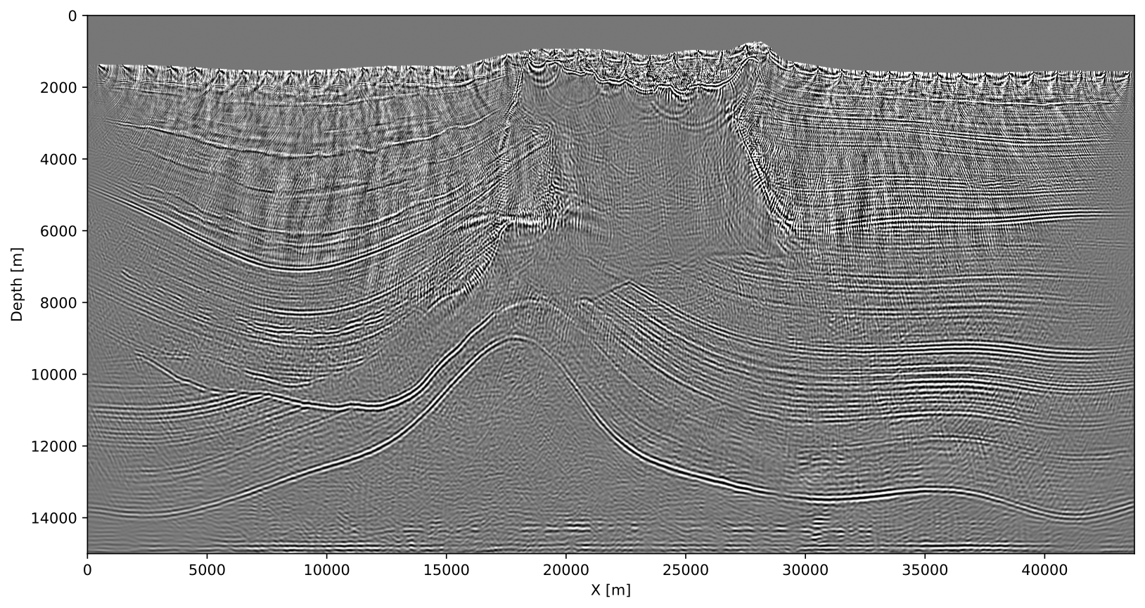
To study the behavior of our approximation on long-offset sparse OBN acquisition, we consider a 2D slice of the SEAM salt model (Fehler and Keliher, 2011). Because this type of acquisition improves the illumination of large salt bodies in the Gulf of Mexico, this type of acquisition has recently gained in popularity. The survey consists of \(44\) OBNs one kilometer apart. At the surface, sources are located every \(12.5m\) at a depth of \(12.5m\). We idealized this dataset by modeling with reciprocity, which leads to \(44\) densely sampled common receiver gathers that serve as input to our approximate imaging approach. As we can clearly see from Figure 2, we are able to produce a good image despite complexity of the model and drastic compression of the wavefield (we use only \(r=64\) probing vectors. Even though we incur limited noise mostly in shallow areas, we argue that these noisy artifacts can easily be removed. At greater depth, the imprint of the noise is less leading to good resolution below the salt.
2007 BP TTI
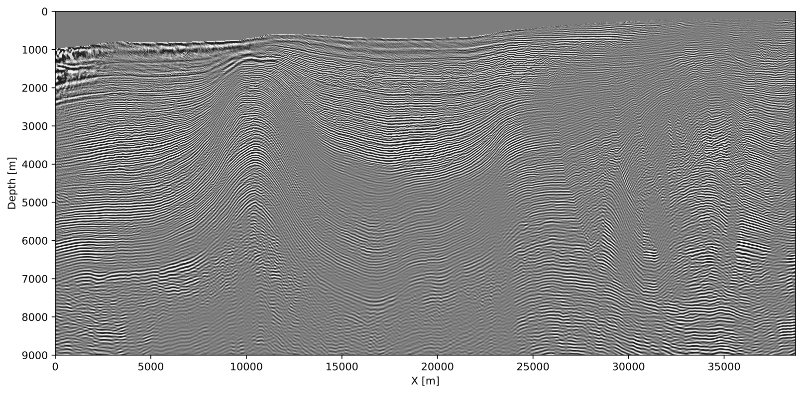
To demonstrate that the proposed method can be extended to more complex imaging physics, we also included an anisotropic example where a subset of the 2007 BP TTI dataset is imaged. Figure 3 includes the imaging result. From this image, we observe that all the layers are imaged correctly and continuously. Because we have a much denser acquisition in this case, the noise incurred by the randomized trace estimation mostly stacks out leading to a very clean image for a fraction of the memory cost of standard RTM. Again all calculations were done exclusively on the GPU.
Code availability
Our implementation and examples are available as open-source software at TimeProbeSeismic.jl, which extends our Julia inversion framework JUDI.jl(P. A. Witte et al., 2019a). Our code is also designed to generalize to 3D and more complicated physics as supported by Devito (Louboutin et al., 2019, Luporini et al. (2020)).
Discussion and conclusions
We presented a proof of concept of wave-based seismic inversion with randomized trace estimation. Aside from demonstrating that this method leads to drastic memory reductions that allow us to form subsurface-offset gathers while remaining on GPUs, we also showed that the incoherent imaging artifacts related to the approximation mostly stack out as long as the fold is sufficient. This allowed us to create high-fidelity images, including subsurface-offset volumes, for realistic anisotropic models with salt. We expect that the reliance on fold can be relaxed when carrying sparsity-promoting imaging or full-waveform inversion with constraints. More importantly, the achieved memory reductions open the way to carry our wave-based inversions (both reverse-time migration and full-waveform inversion) exclusively on GPUs without the need to delicate certain tasks to CPUs. This capability opens the perspective of carrying out industry-scale 3D wave-based inversions with domain decomposition on clusters of GPUs. As long as these GPUs are connected with a low-latency network fabric, we expect a major boost in performance thanks to exclusive use of accelerators facilitated by the reduction in memory footprint.
Acknowledgement
This research was carried out with the support of Georgia Research Alliance and partners of the ML4Seismic Center.
References
Avron, H., and Toledo, S., 2011, Randomized algorithms for estimating the trace of an implicit symmetric positive semi-definite matrix: J. ACM, 58. doi:10.1145/1944345.1944349
Fehler, M., and Keliher, P. J., 2011, SEAM Phase I: Challenges of Subsalt Imaging in Tertiary Basins, with Emphasis on Deepwater Gulf of Mexico: Society of Exploration Geophysicists. doi:10.1190/1.9781560802945
Friedlander, M. P., and Schmidt, M., 2012, Hybrid deterministic-stochastic methods for data fitting: SIAM Journal on Scientific Computing, 34, A1380–A1405. doi:10.1137/110830629
Graff-Kray, M., Kumar, R., and Herrmann, F. J., 2017, Low-rank representation of omnidirectional subsurface extended image volumes:. SINBAD. Retrieved from https://slim.gatech.edu/Publications/Public/Conferences/SINBAD/2017/Fall/graff2017SINBADFlrp/graff2017SINBADFlrp.pdf
Griewank, A., and Walther, A., 2000, Algorithm 799: Revolve: An implementation of checkpointing for the reverse or adjoint mode of computational differentiation: ACM Trans. Math. Softw., 26, 19–45. doi:10.1145/347837.347846
Haber, E., Doel, K. van den, and Horesh, L., 2015, Optimal design of simultaneous source encoding: Inverse Problems in Science and Engineering, 23, 780–797. doi:10.1080/17415977.2014.934821
Krebs, J. R., Anderson, J. E., Hinkley, D., Baumstein, A., Lee, S., Neelamani, R., and Lacasse, M., 2009a, Fast full wave seismic inversion using source encoding: In SEG technical program expanded abstracts 2009 (pp. 2273–2277). doi:10.1190/1.3255314
Krebs, J. R., Anderson, J. E., Hinkley, D., Neelamani, R., Lee, S., Baumstein, A., and Lacasse, M.-D., 2009b, Fast full-wavefield seismic inversion using encoded sources: GEOPHYSICS, 74, WCC177–WCC188. doi:10.1190/1.3230502
Kukreja, N., Hückelheim, J., Louboutin, M., Washbourne, J., Kelly, P. H. J., and Gorman, G. J., 2020, Lossy checkpoint compression in full waveform inversion: Geoscientific Model Development Discussions, 2020, 1–26. doi:10.5194/gmd-2020-325
Leeuwen, T. van, and Herrmann, F. J., 2013, Fast waveform inversion without source-encoding: Geophysical Prospecting, 61, 10–19. doi:https://doi.org/10.1111/j.1365-2478.2012.01096.x
Leeuwen, T. van, Kumar, R., and Herrmann, F. J., 2017, Enabling affordable omnidirectional subsurface extended image volumes via probing: Geophysical Prospecting, 65, 385–406. doi:10.1111/1365-2478.12418
Lions, J. L., 1971, Optimal control of systems governed by partial differential equations: (1st ed.). Springer-Verlag Berlin Heidelberg.
Louboutin, M., and Herrmann, F. J., 2021, Ultra-low memory seismic inversion with randomized trace estimation: SEG technical program expanded abstracts. doi:10.1190/segam2021-3584072.1
Louboutin, M., Lange, M., Luporini, F., Kukreja, N., Witte, P. A., Herrmann, F. J., … Gorman, G. J., 2019, Devito (v3.1.0): An embedded domain-specific language for finite differences and geophysical exploration: Geoscientific Model Development, 12, 1165–1187. doi:10.5194/gmd-12-1165-2019
Luporini, F., Louboutin, M., Lange, M., Kukreja, N., Witte, P., Hückelheim, J., … Gorman, G. J., 2020, Architecture and performance of devito, a system for automated stencil computation: ACM Trans. Math. Softw., 46. doi:10.1145/3374916
McMechan, G. A., 1983, MIGRATION bY eXTRAPOLATION oF tIME-dEPENDENT bOUNDARY vALUES: Geophysical Prospecting, 31, 413–420. doi:10.1111/j.1365-2478.1983.tb01060.x
Meyer, R. A., Musco, C., Musco, C., and Woodruff, D. P., 2020, Hutch++: Optimal Stochastic Trace Estimation: ArXiv E-Prints, arXiv:2010.09649.
Mittet, R., 1994, Implementation of the kirchhoff integral for elastic waves in staggered-grid modeling schemes: GEOPHYSICS, 59, 1894–1901. doi:10.1190/1.1443576
Moghaddam, P. P., Keers, H., Herrmann, F. J., and Mulder, W. A., 2013, A new optimization approach for source-encoding full-waveform inversion: GEOPHYSICS, 78, R125–R132. doi:10.1190/geo2012-0090.1
Raknes, E. B., and Weibull, W., 2016, Efficient 3D elastic full-waveform inversion using wavefield reconstruction methods: Geophysics, 81, R45–R55. doi:10.1190/geo2015-0185.1
Romero, L. A., Ghiglia, D. C., Ober, C. C., and Morton, S. A., 2000, Phase encoding of shot records in prestack migration: GEOPHYSICS, 65, 426–436. doi:10.1190/1.1444737
Symes, 2007, Reverse time migration with optimal checkpointing: GEOPHYSICS, 72, SM213–SM221. doi:10.1190/1.2742686
Symes, W. W., 2008, Migration velocity analysis and waveform inversion: Geophysical Prospecting, 56, 765–790. doi:https://doi.org/10.1111/j.1365-2478.2008.00698.x
Tarantola, A., 1984, Inversion of seismic reflection data in the acoustic approximation: GEOPHYSICS, 49, 1259. doi:10.1190/1.1441754
Thomsen, L., 1986, Weak elastic anisotropy: Geophysics, 51, 1964–1966.
Trefethen, L. N., and Bau III, D., 1997, Numerical linear algebra: (1st ed.). Siam.
Virieux, J., and Operto, S., 2009, An overview of full-waveform inversion in exploration geophysics: GEOPHYSICS, 74, WCC1–WCC26. doi:10.1190/1.3238367
Witte, P. A., Louboutin, M., Kukreja, N., Luporini, F., Lange, M., Gorman, G. J., and Herrmann, F. J., 2019a, A large-scale framework for symbolic implementations of seismic inversion algorithms in julia: GEOPHYSICS, 84, F57–F71. doi:10.1190/geo2018-0174.1
Witte, P. A., Louboutin, M., Luporini, F., Gorman, G. J., and Herrmann, F. J., 2019b, Compressive least-squares migration with on-the-fly fourier transforms: Geophysics, 84, R655–R672. doi:10.1190/geo2018-0490.1
Yang, M., Graff, M., Kumar, R., and Herrmann, F. J., 2021, Low-rank representation of omnidirectional subsurface extended image volumes: Geophysics, 86, 1–41. doi:10.1190/geo2020-0152.1