Fast Robust Waveform inversion: Examples and results

Scripts to reproduce the famous Camembert example, as well as results from several papers are included. Updated to conform to the new software design outlined in [4].

Contents

Camembert example

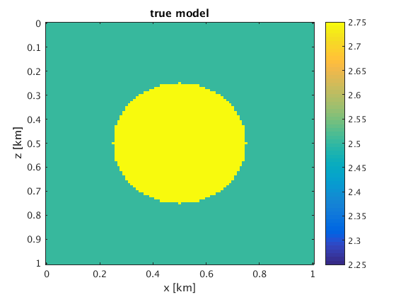
The basic functionality of the waveform inversion code is demonstrated on an example based on the famous `Camembert' model [1]. See the script camembert.m.

% true model
[v,n,d,o] = rsf_read_all([resultsdir '/camembert/vtrue.rsf']);

v  = 1e-3*v;
[z,x] = odn2grid(o,d,n);
z = z*1e-3; x = x*1e-3;

figure;imagesc(x,z,v,[2.25 2.75]);colorbar;
xlabel('x [km]');ylabel('z [km]'); title('true model');

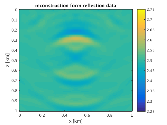
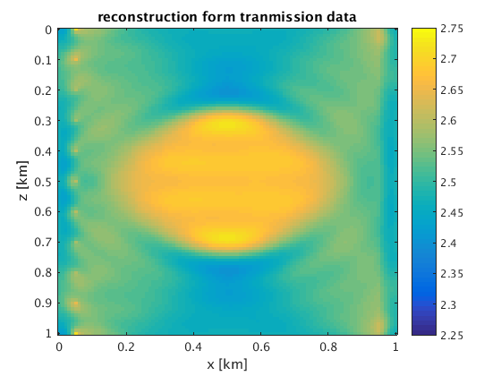
% reconstructions
vnr = rsf_read_all([resultsdir '/camembert/vn_r.rsf']);
vnt = rsf_read_all([resultsdir '/camembert/vn_t.rsf']);
vnr = 1e-3*vnr;
vnt = 1e-3*vnt;

figure;imagesc(x,z,vnr,[2.25 2.75]);colorbar;
xlabel('x [km]');ylabel('z [km]'); title('reconstruction form reflection data');

figure;imagesc(x,z,vnt,[2.25 2.75]);colorbar;
xlabel('x [km]');ylabel('z [km]'); title('reconstruction form tranmission data');

Fast Waveform inversion without source-encoding

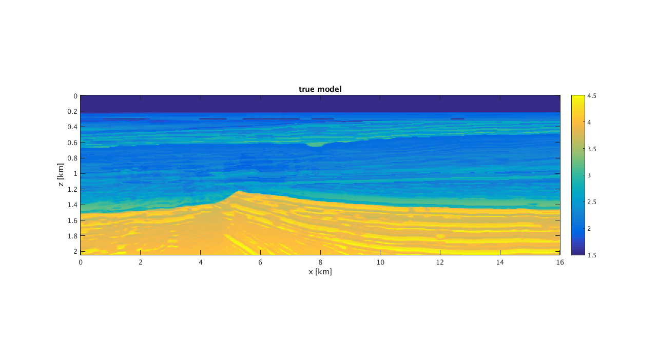
Waveform inversion using stochastic optimization with bound constraints. See the script bg2_batch.m.

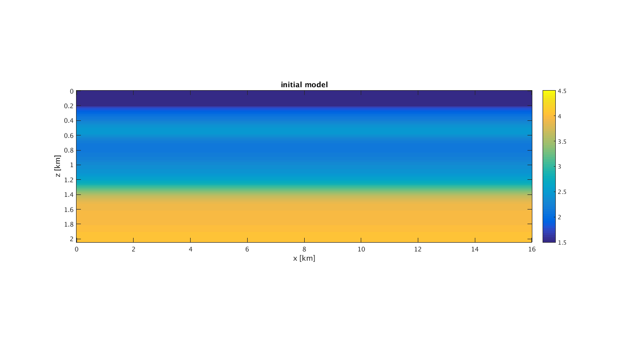
[v,n,d,o] = rsf_read_all([datadir '/bg2v.rsf']);
[v0,n,d,o] = rsf_read_all([datadir '/bg2v0.rsf']);

v  = 1e-3*v;
v0 = 1e-3*v0;
[z,x] = odn2grid(o,d,n);
z = z*1e-3; x = x*1e-3;

scnsize = get(0,'ScreenSize');

% The true and initial model
%

figure('Position',scnsize./[1 1 2 2]);imagesc(x,z,v,[1.5 4.5]);colorbar;set(gca,'plotboxaspectratio',[3 1 1]);
xlabel('x [km]');ylabel('z [km]'); title('true model');

figure('Position',scnsize./[1 1 2 2]);imagesc(x,z,v0,[1.5 4.5]);colorbar;set(gca,'plotboxaspectratio',[3 1 1]);
xlabel('x [km]');ylabel('z [km]'); title('initial model');

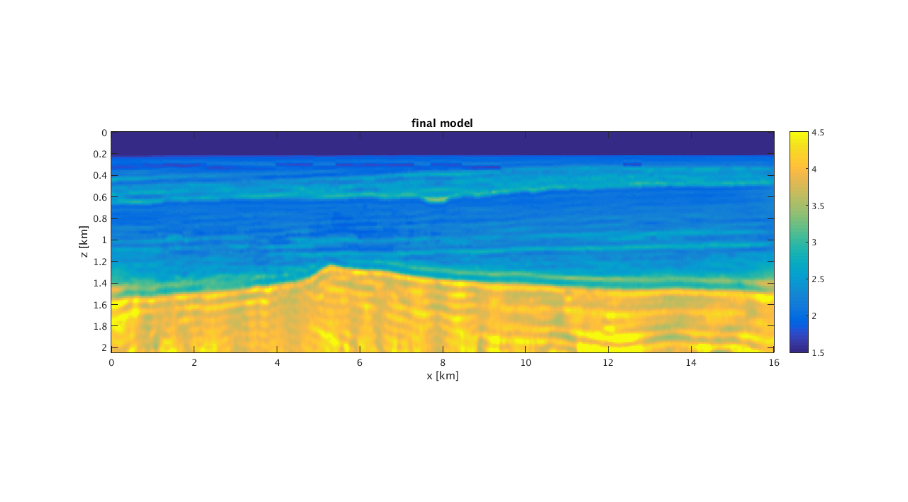
reconstruction with batching after 17th. frequency band.

[mn,n,d,o] = rsf_read_all([resultsdir '/bg2_batch/mn_17.rsf']);
vn = real(1./sqrt(mn));

figure('Position',scnsize./[1 1 2 2]);imagesc(x,z,vn,[1.5 4.5]);colorbar;set(gca,'plotboxaspectratio',[3 1 1]);
xlabel('x [km]');ylabel('z [km]'); title('final model');

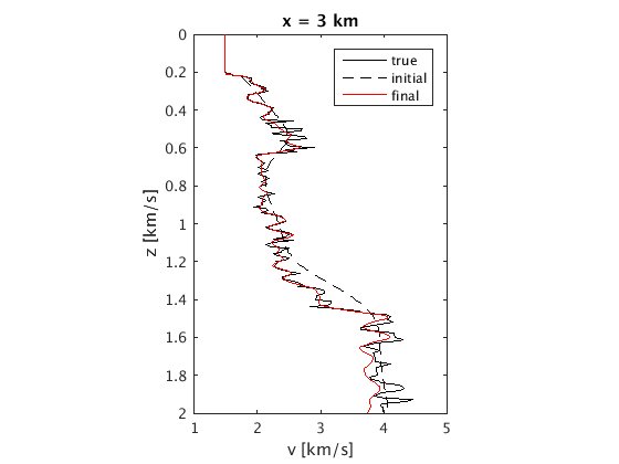
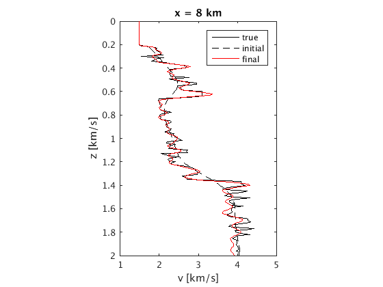
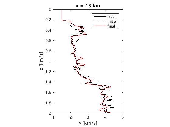
xslices = [3 8 13];
for i=1:length(xslices)
    ix = x==xslices(i);
    figure;plot(v(:,ix),z,'k',v0(:,ix),z,'k--',vn(:,ix),z,'r');axis ij; ylim([0 2]);set(gca,'plotboxaspectratio',[1 1.5 1]);
    xlabel('v [km/s]');ylabel('z [km/s]');title(['x = ' num2str(xslices(i)) ' km']);legend('true','initial','final');
end

Robust waveform inversion with source estimation

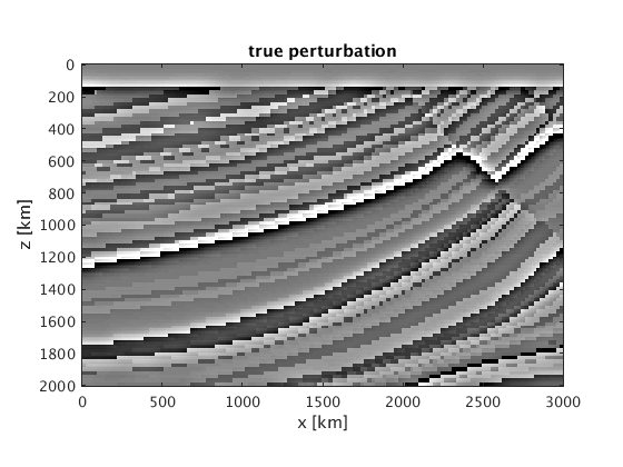
Robust waveform inversion with robust source estimation [3].

[v, n,d,o] = rsf_read_all([datadir 'marmv.rsf']);
[v0,n,d,o] = rsf_read_all([datadir 'marmv0.rsf']);

[z,x] = odn2grid(o,d,n);

m  = 1e6./v.^2;
m0 = 1e6./v0.^2;

figure;imagesc(x,z,m-m0,[-1 1]*5e-2);axis equal tight;colormap(gray);
xlabel('x [km]');ylabel('z [km]'); title('true perturbation');

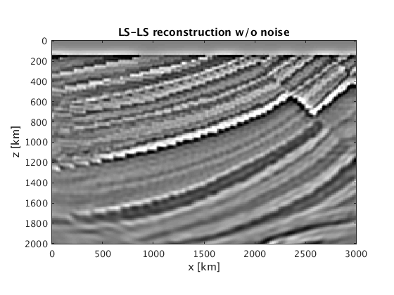
A LS-LS reconstruction without outliers looks like this. See mbase.m.

[mbase] = rsf_read_all([resultsdir '/mbase/mn.rsf']);

figure;imagesc(x,z,mbase-m0,[-1 1]*5e-2);axis equal tight;colormap(gray);
xlabel('x [km]');ylabel('z [km]'); title('LS-LS reconstruction w/o noise');

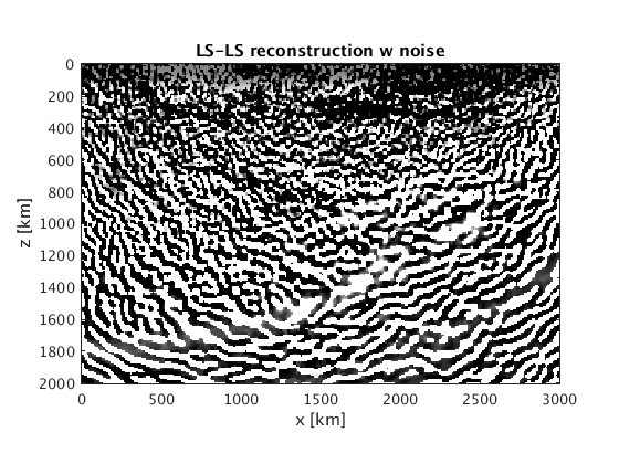
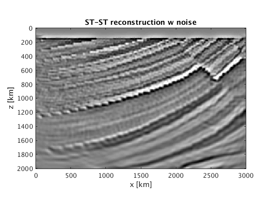
Reconstructions with outliers using LS-LS, or ST-ST, see mlsls.m and mstst.m.

[mlsls] = rsf_read_all([resultsdir '/mlsls/mn.rsf']);
[mstst] = rsf_read_all([resultsdir '/mstst/mn.rsf']);


figure;imagesc(x,z,mlsls-m0,[-1 1]*5e-2);axis equal tight;colormap(gray);
xlabel('x [km]');ylabel('z [km]'); title('LS-LS reconstruction w noise');

figure;imagesc(x,z,mstst-m0,[-1 1]*5e-2);axis equal tight;colormap(gray);
xlabel('x [km]');ylabel('z [km]'); title('ST-ST reconstruction w noise');

References

[1] O. Gauthier, J. Virieux, and A. Tarantola. Two-dimensional nonlinear inversion of seismic waveforms: Numerical results. Geophysics 51, 1387-1403 (1986)

[2] T. van Leeuwen and F.J. Herrmann - Fast Waveform inversion without source-encoding, Geophysical Prospecting, submitted

[3] A.Y. Aravkin, T. van Leeuwen and F.J. Herrmann - Source estimation for frequency-domain FWI with robust penalties, EAGE Expanded abstracts 2012.

[4] C. Da Silva, F.J. Herrmann - A unified 2D/3D software environment for large scale time-harmonic full waveform inversion.

Acknowledgements

The synthetic Compass model was provided by the BG-GROUP, see also the disclaimer.