Seismic Trace Interpolation: Examples and results
Scripts to reproduce the reconstruction results found in [1].
Contents
Reconstruction in the midpoint-offset domain
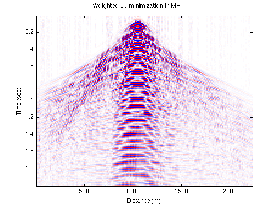
The basic functionality of the trace interpolation code is demonstrated on an example seismic line from the Gulf of Suez. The seismic waveform continuity is exploited across frequency slices in the midpoint offset domain. See the script wL1_freq_MH.m.
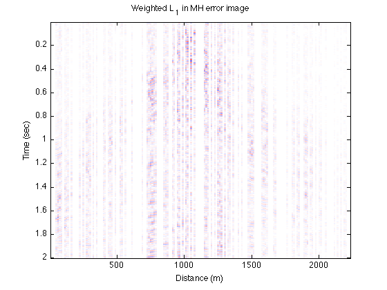
Reconstruction using weighted L1 minimization
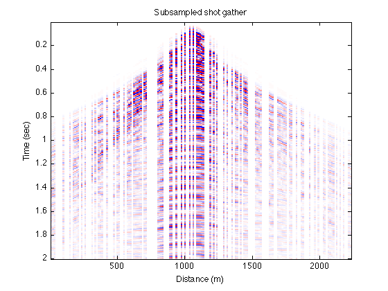
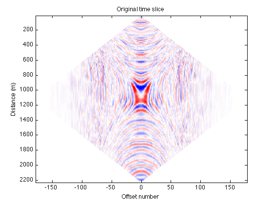
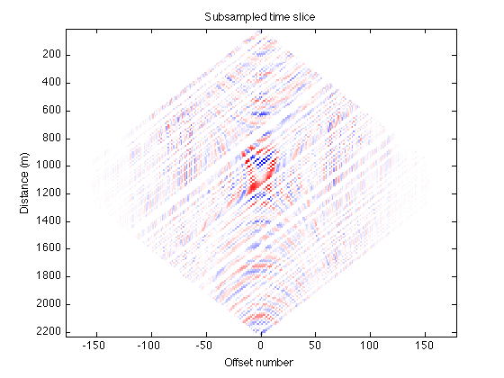
% Load the data from the output directory
label = 'wL1FreqMH';
datadir = '../data/';
outputdir = ['../results/' label];
load([outputdir, '/wL1_freq_MH.mat']);

% original and subsampled shot gather
shot_num = 84;

dim = size(D);
DSG = reshape(D(:,:,shot_num),dim(1),dim(2));
DSG_sub = zeros(dim(1),dim(2));
DSG_sub(:,mask(:,1)) = DSG(:,mask(:,1));
figure;
imagesc([1:dim(2)]*12.5, [1:dim(1)]*4e-3,DSG);colormap(seiscol); caxis([-50 50])
title('Original shot gather'); xlabel('Distance (m)'); ylabel('Time (sec)');
figure;
imagesc([1:dim(2)]*12.5, [1:dim(1)]*4e-3,DSG_sub);colormap(seiscol); caxis([-50 50])
title('Subsampled shot gather'); xlabel('Distance (m)'); ylabel('Time (sec)');


% Original and subsampled time slice
time = 350;
dim = size(DH);
DHt = reshape(DH(time,:,:),dim(2), dim(3));

figure; imagesc([-dim(2):dim(2)], [1:dim(2)]*12.5,DHt); colormap(seiscol); caxis([-50, 50])
title('Original time slice'); xlabel('Offset number'); ylabel('Distance (m)');
figure; imagesc([-dim(2):dim(2)], [1:dim(2)]*12.5,DHt.*maskH); colormap(seiscol); caxis([-50, 50])
title('Subsampled time slice'); xlabel('Offset number'); ylabel('Distance (m)');

% Weighted L1 reconstructed shot gather
dim = size(Dest);
DestSG = reshape(Dest(:,:,shot_num),dim(1),dim(2));

figure;
imagesc([1:dim(2)]*12.5, [1:dim(1)]*4e-3,DestSG);colormap(seiscol); caxis([-50 50])
title('Weighted L_1 minimization in MH'); xlabel('Distance (m)'); ylabel('Time (sec)');

Err_wl1MH = DSG - DestSG;
figure; imagesc([1:dim(2)]*12.5, [1:dim(1)]*4e-3,(Err_wl1MH));colormap(seiscol); caxis([-50 50])
title('Weighted L_1 in MH error image'); xlabel('Distance (m)'); ylabel('Time (sec)');

% compute shot gather relative error
for s = 1:dim(2)
    EwL1freqMH_source(s) = norm(vec(D(:,:,s)) - vec(Dest(:,:,s)))/norm(vec(D(:,:,s)));
end

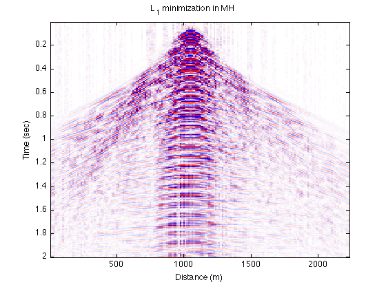
Reconstruction using L1 minimization
Load L1 data from output directory
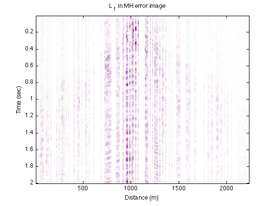
label = 'L1FreqMH';
datadir = '../data/';
outputdir = ['../results/' label];
load([outputdir, '/L1_freq_MH.mat']);

% L1 reconstructed shot gather
dim = size(Dest);
DestSG = reshape(Dest(:,:,shot_num),dim(1),dim(2));

figure;
imagesc([1:dim(2)]*12.5, [1:dim(1)]*4e-3,DestSG);colormap(seiscol); caxis([-50 50])
title('L_1 minimization in MH'); xlabel('Distance (m)'); ylabel('Time (sec)');

Err_l1MH = DSG - DestSG;
figure; imagesc([1:dim(2)]*12.5, [1:dim(1)]*4e-3,(Err_l1MH));colormap(seiscol); caxis([-50 50])
title('L_1 in MH error image'); xlabel('Distance (m)'); ylabel('Time (sec)');

% compute shot gather relative error
for s = 1:dim(2)
    EL1freqMH_source(s) = norm(vec(D(:,:,s)) - vec(Dest(:,:,s)))/norm(vec(D(:,:,s)));
end
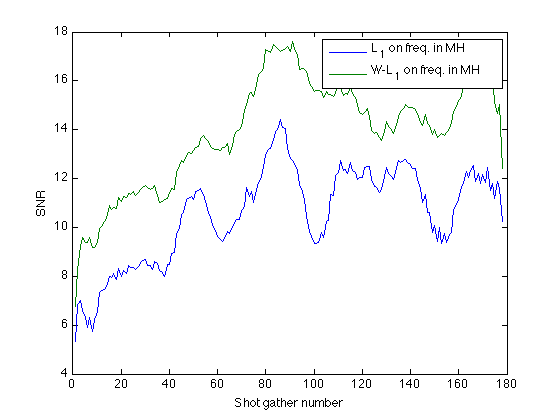
Compare shot gather SNRs
figure; plot( 1:dim(2), -20*log10(EL1freqMH_source), 1:dim(2), -20*log10(EwL1freqMH_source));
legend('L_1 on freq. in MH', 'W-L_1 on freq. in MH'); xlabel('Shot gather number'); ylabel('SNR')