Compressive least-squares migration with source estimation

Introduction

Reverse-time migration (RTM) is an increasingly popular wave-equation based seismic imaging algorithm that corresponds to applying the adjoint of the Born scattering operator to observed reflection data (Baysal et al., 1983; Whitmore, 1983). Without extensive preconditioning, applying the adjoint operator leads to an image with incorrect amplitudes, imprints of the source wavelet and therefore blurred reflectors. To overcome these issues, imaging can be formulated as a linear least-squares optimization problem, in which the mismatch between observed and modeled data is minimized (Schuster, 1993; Nemeth et al., 1999; Dong et al., 2012; Zeng et al., 2014). Conventional LS-RTM is computationally very expensive, because it requires migration and demigration of all shot records during each iteration. To save computational resources, shots can be subsampled or combined into simultaneous shots, which avoids having to treat every shot separately in each iteration (e.g. Romero et al., 2000; Tang and Biondi, 2009; Leeuwen et al., 2011; Dai et al., 2011, 2012; Liu, 2013; Herrmann and Li, 2012; Lu et al., 2015).

An RTM image or LS-RTM gradient is calculated by forward modeling the source wavelet in the background model, backpropagating the observed data or data residual and applying an imaging condition. The source wavelet is generally unknown and therefore needs to be estimated prior to imaging or as part of the inversion process. Source estimation has been proposed in the context of frequency domain full-waveform inversion (FWI) (Pratt, 1999; Aravkin et al., 2012) and frequency domain LS-RTM (Tu et al., 2013), where a single complex number per frequency needs to be estimated. In the time domain, we are only aware of the work of Zhang et al. (2016), who formulate LS-RTM independently of the source wavelet, i.e. they eliminate the wavelet from the objective and minimize the misfit between the predicted and true Green’s functions. To our knowledge, there are no algorithms so far that combine time-domain LS-RTM and estimation of the full time-dependent source function.

We introduce an algorithm that addresses the two main challenges of time-domain LS-RTM: estimating the source wavelet and decreasing the overall computational cost. We extend our earlier work on sparsity-promoting imaging (SPLS-RTM) and FWI in the frequency domain (Li et al., 2012; Herrmann et al., 2015; Tu and Herrmann, 2015) and adapt an algorithm that has recently gained popularity in the context of compressive sensing. The linearized Bregman method (Yin, 2010) is an algorithm for recovering the sparse solution of an underdetermined linear system, which is closely related to the iterative soft-thresholding algorithm (ISTA). However, it has been mathematically shown that the algorithm can also be used to solve overdetermined linear systems and allows working with subsets of rows and data points in each iteration (Lorenz et al., 2014b). This means that during each LS-RTM iteration, we model and migrate only a small subset of randomly selected shots instead of the full data set and still converge to the true solution. The algorithm is simple to implement and in contrast to ISTA requires only a single and relatively easy to choose hyperparameter. Furthermore we incorporate source estimation via variable projection into this algorithm, which lets us estimate the source wavelet without additional PDE solves.

The linearized Bregman method for SPLS-RTM

In a series of previous publications (e.g. Herrmann and Li (2012), Tu and Herrmann (2015)), we have reformulated LS-RTM as a sparsity-promoting least-squares minimization problem of the following form: \[ \begin{equation} \begin{aligned} &\underset{\mathbf{\delta m}}{\operatorname{minimize}} \hspace{0.4cm} \| \mathbf{C} \hspace{.1cm} \mathbf{\delta m}\|_1 \\ &\text{subject to } \|\hspace{0.1cm} \nabla \textbf{F}\big(\mathbf{m}_0, \mathbf{q} \big) \mathbf{\delta m} - \mathbf{\delta d}\|_2 \leq \sigma. \end{aligned} \label{bpdn} \end{equation} \] These optimization problems are called basis pursuit denoise (BPDN) problems and have recently gained large popularity in the context of compressive sensing (Donoho, 2006). The objective of this problem is to minimize the \(\ell_1\)-norm of the curvelet coefficients of the seismic image \(\mathbf{\delta m}\), obtained through the forward Curvelet transform \(\mathbf{C}\). This is subject to the constraint that the synthetic data, given by the action of the Born modeling operator \(\nabla \mathbf{F}\) on \(\mathbf{\delta m}\), fits the observed reflections \(\mathbf{\delta d}\) within some noise level \(\sigma\). The Born modeling operator is a function of the background velocity model \(\mathbf{m}_0\) and the source wavelet \(\mathbf{q}\), which are for now assumed to be known. As shown in Li et al. (2012), enforcing sparsity on the seismic image leads to high quality results when working with randomization techniques, where the computational cost of LS-RTM can be significantly reduced by working with randomized subsets of sources during each iteration.

The main drawback of this approach is that optimization algorithms that solve the BPDN problem, such as the spectral projected gradient method with \(\ell_1\) (SPG\(\ell_1\)) (van den Berg and Friedlander, 2008) are difficult to implement and do not necessarily allow us to work with randomization techniques. Other solvers such as ISTA, work with modifications of the BPDN problem and solve an unconstrained formulation in which the constraint is added to the objective as a penalty. This introduces a penalty parameter that is difficult to choose and requires complex cooling techniques (i.e. the penalty parameter needs to be relaxed) in order to converge to the solution sufficiently quickly (Hennenfent et al., 2008).

An alternative algorithm, which has recently gained popularity in solving sparsity-promoting least-squares problems is the linearized Bregman method (Yin, 2010). The algorithm solves a slightly modified version of the BPDN problem, in which an \(\ell_2\) penalty term is added to the objective:: \[ \begin{equation} \begin{aligned} &\underset{\mathbf{\delta m}}{\operatorname{minimize}} \hspace{0.4cm} \lambda \|\mathbf{C} \hspace{.1cm} \mathbf{\delta m}\|_1 + \frac{1}{2}\|\mathbf{C} \hspace{.1cm} \mathbf{\delta m} \|^2_2 \\ &\text{subject to } \|\hspace{0.1cm} \nabla \textbf{F}\big(\mathbf{m}_0, \mathbf{q}\big) \mathbf{\delta m} - \mathbf{\delta d}\|_2 \leq \sigma. \end{aligned} \label{lb} \end{equation} \] The combination of \(\ell_1\)- and \(\ell_2\)-norm terms in the objective is referred to as an elastic net in machine learning and has the effect of making the objective function strongly convex (Lorenz et al., 2014a). This small change to the objective yields a relatively simple iterative scheme for minimizing the above optimization problem, in which the penalty parameter \(\lambda\) plays a completely different role than in ISTA. In ISTA, \(\lambda\) is a penalty parameter that controls the trade-off between the \(\ell_1\)-norm of the (transform-domain) image and the data fidelity term and to solve the BPDN problem, we need \(\lambda \rightarrow 0^+\) (i.e. \(\lambda\) goes to 0 from above). However, as discussed in Hennenfent et al. (2008), small values of \(\lambda\) lead to very slow convergence of ISTA and complex cooling techniques are required to improve its performance. A value of \(\lambda\) that is too large on the other hand, prevents any entries in the unknown to enter into the solution. In the linearized Bregman method on the other hand, \(\lambda\) controls the trade-off between the \(\ell_1\)- and \(\ell_2\)-norms of the unknown model vector. A value of \(\lambda\) that is too large only initially prevents new entries to enter into the solution, but as the iterations progress, larger and larger values start entering the solution, making the algorithm in some sense “self-tuning” (Herrmann et al., 2015). Choosing an appropriate value for \(\lambda\) in the linearized Bregman method is therefore easier and can be done automatically. For example, setting \(\lambda\) to the infinity norm of the gradient in the first iteration, leads to no value passing the first threshold, but the solution starts to build up from iteration two onwards.

Another important benefit of the linearized Bregman method is the possibility to work with subsets of blocks of rows of \(\nabla \mathbf{F}\) (each corresponding to a source experiment) and \(\mathbf{\delta d}\) during each iteration, while still converging to the correct solution (Lorenz et al., 2014b). For least-squares migration, this means that instead of treating all shot records during each iteration, we can use a randomized subset of fewer source positions, thus decreasing the number of PDE solves. This provides flexibility to the user to find a trade-off between the number of sources per iteration and the overall number of iterations. In the extreme case, it is possible to use only a single shot in each iteration, which then requires many iterations to reach an acceptable solution. We found that it is often sufficient to use between \(\sim \frac{1}{10}\) and \(\frac{1}{20}\) of the shots during each iteration and perform around \(\sim 20\) overall iterations, i.e. on average every shot record is demigrated/migrated only once or twice, making our algorithm in terms of PDE solves several times cheaper than conventional LS-RTM.

On-the-fly source estimation

The algorithm in the previous section assumes that the source wavelet \(\mathbf{q}\) is known, which is generally not the case. Often some general information about the source function is known, i.e. the approximate frequency range, the general wavelet shape and the approximate length in time. We therefore base our source estimation algorithm on the assumption that an initial guess of the true wavelet \(\mathbf{q}_0\) is available and that there exists a filter \(\mathbf{w}\), such that convolving the initial guess with this filter yields the correct source wavelet: \(\mathbf{q} = \mathbf{q}_0 \ast \mathbf{w}\), with the symbol \(\ast\) denoting circular convolution over time. SPLS-RTM with source estimation can then be formulated as a multi-parameter optimization problem with the image \(\mathbf{\delta m}\) and the filter \(\mathbf{w}\) as unknowns. Optimization problems of this form require gradients of the objective with respect to both parameters, which not only requires a completely new optimization algorithm, but can also pollute the image during the early iterations, as the initial wavelet might be far off from the true one. We therefore follow the approach in Aravkin et al. (2012) and Tu et al. (2013) and formulate the objective as a separable least-squares problem, which can be solved using the variable projection method (Golub and Pereyra, 2003). For this, we only replace the Jacobian in equation \(\ref{lb}\) by \(\mathbf{w} ( \mathbf{\delta m} ) \ast [ \nabla \textbf{F} (\mathbf{m}_0, \mathbf{q}_0 ) \delta \mathbf{m} ]\). This corresponds to modeling the data with the initial source wavelet \(\mathbf{q}_0\), followed by a trace-by-trace convolution with the filter \(\mathbf{w}(\mathbf{\delta m})\). The filter is a function of the current estimate of the image and is obtained by solving a small independent least-squares subproblem during each iteration: \[ \begin{equation} \mathbf{w}_k = \underset{\mathbf{w}}{\operatorname{argmin}} \| \mathbf{w} \ast \Big[ \nabla \mathbf{F}_k \big(\mathbf{m}_0, \mathbf{q}_0\big) \mathbf{\delta m}_k \Big] - \mathbf{\delta d}_k \|^2. \label{qest} \end{equation} \] As mentioned earlier, we want to work with randomized subsets of shots during each iteration, so \(\mathbf{\nabla F}_k\) and \(\delta \mathbf{d}_k\) denote the subset of the Jacobian and the data at the current iteration \(k\) and \(\mathbf{\delta m}_k\) is the current estimate of the image. We want the estimated wavelet to be localized in time, since we know that the time signature of an impulsive source is typically short. Therefore the vector \(\mathbf{w}\) for the filter is chosen to have the approximate length of the true wavelet.

The algorithm for time-domain SPLS-RTM with source estimation is outlined below. Each iteration involves choosing a randomized subset of shots and \(\mathbf{\nabla F}_k\) and \(\mathbf{\delta d}_k\) denote the current subset of the Jacobian and the data (lines \(3-5\)). Updating the gradient (line \(8\)) requires a step size, which is chosen as \(t_k = \|\mathbf{w}_k \ast \mathbf{d}_k - \widehat{\mathbf{\delta d}_k}\|/ \| \mathbf{\nabla F}^\top \big( \mathbf{w}_k \ast \mathbf{d}_k - \widehat{\mathbf{\delta d}_k} \big)\|\) (Lorenz et al., 2014b). The operator \(\mathcal{P}_\sigma\) in line \(8\) is a projection operator that projects the data residual onto the \(\ell_2\)-ball of the size of the noise, i.e. it does not fit the data exactly. Calculating the gradient also involves the transpose action of the convolution operator (line \(8\)), which is the correlation of \(\mathbf{w}_k\) with the data (denoted by \(\star\)). The function \(S_\lambda\) (line 9) is the soft thresholding function.

Numerical example

We test our algorithm for SPLS-RTM with source estimation on the Sigsbee 2A velocity model (Bashkardin et al., 2002) and show that our proposed algorithm is capable of accurately recovering the source wavelet and provides a high quality image with good illumination below the salt, while only requiring two passes through the data. We generate linearized observed data for 960 source locations with 25 m shot spacing and 10 seconds recording time. Each shot is recorded by 960 receivers, located at 25 m depth with a maximum offset of 10 km. We use a minimum phase source wavelet to generate the synthetic observed data with 15 Hz peak frequency (shown in figure 1).

For SPLS-RTM with source estimation, we have to define an initial wavelet from which the true wavelet can be estimated reliably with our algorithm. We found this is the case for an initial wavelet with a wide frequency spectrum, meaning the initial wavelet contains a broad range of frequencies, while the shape of the spectrum, as well as the phase can be well recovered with our algorithm. We design the spectrum of the initial wavelet to have a plateau between 15-25 Hz, which is wider than the approximate peak frequency of the true wavelet. To show that we can recover the true source from an initial wavelet with a different phase and shape, we design the initial wavelet to be mixed-phase with various side lobes, while the true wavelet is minimum phase (figure 1).

For SPLS-RTM with and without source estimation we run 18 iterations of the linearized Bregman method with 100 sources per iteration, which corresponds to roughly two passes through the data. Our velocity model is a smoothed version of the true model, meaning it is kinematically correct. We use a few basic preconditioners to improve the convergence of our algorithm. In the model domain, we use a linear depth scaling preconditioner, as well as a topmute to remove the source/receiver imprints in the water column. In the data domain, we employ a data topmute to suppress the water bottom reflection, as well as a half integration to compensate for the order of the 2D normal operator (Herrmann et al., 2008). One challenge of the Sigsbee 2A model is the strong and shallow salt body, which causes significant backscattering of the forward modeled wavefield and leads to low-frequency artifacts in the gradients. We address this problem by using the linearized inverse scattering imaging condition (Op’t Root et al., 2012; Whitmore and Crawley, 2012) instead of the crosscorrelation imaging condition. This modification is incorporated into both the imaging operator \(\mathbf{\nabla F}^\top\) and the modeling operator \(\mathbf{\nabla F}\), in order to preserve their adjointness (Witte et al., 2017). The only hyperparameter we need to choose is \(\lambda\), which we set according to the maximum absolute value of the gradient in the first iteration, as mentioned in the theory section. We set \(\lambda\) to the \(\frac{1}{10}\) of the maximum absolute value, which leads to values already entering the solution during the first iteration. We found that setting \(\lambda\) to be larger than this, requires too many iterations to build up an image that includes also the small amplitude reflectors.

Discussion

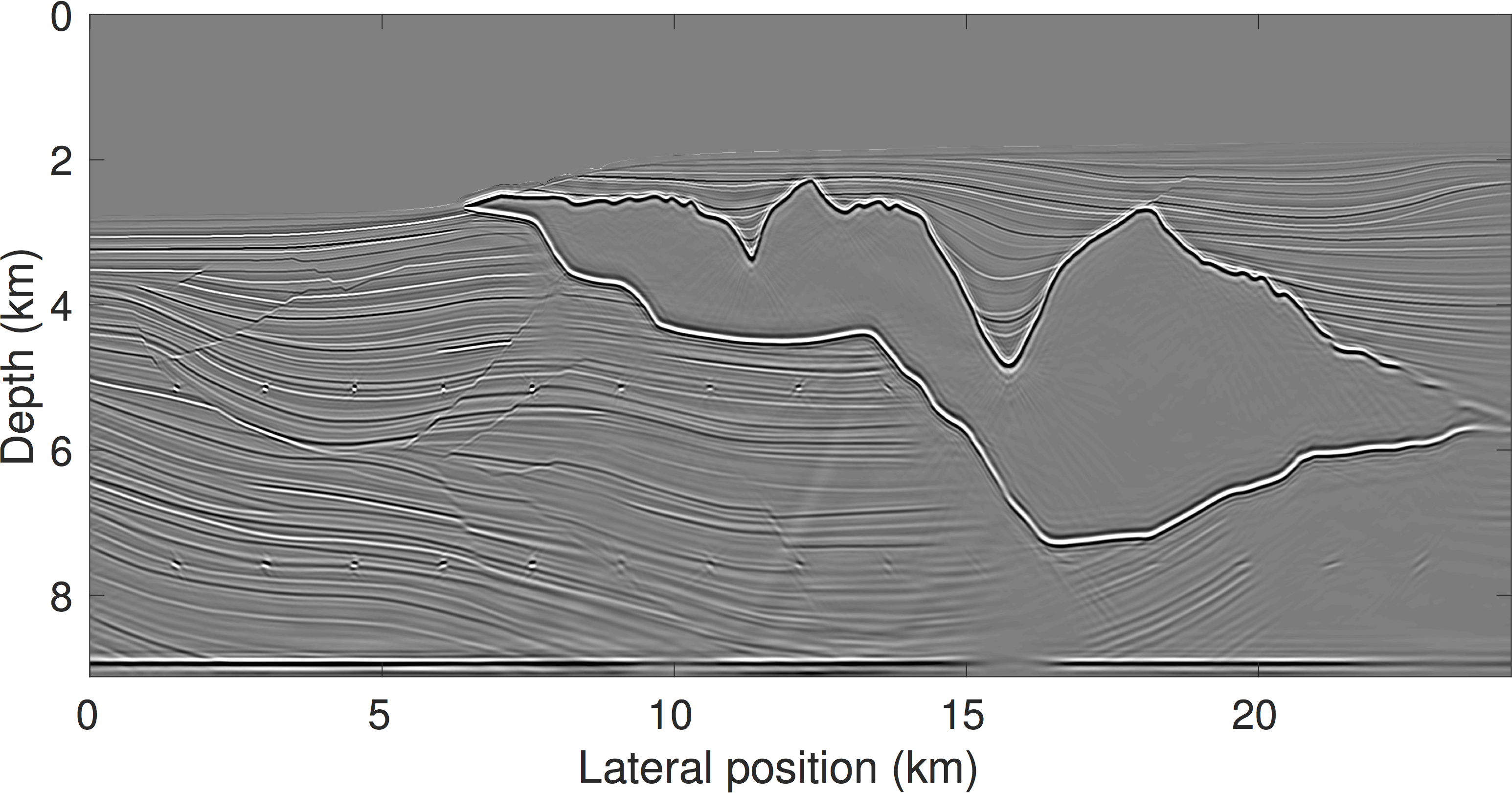
Figures 2 and 3 show the conventional RTM image in comparison to the result after 18 iterations. The RTM image was obtained using the true source wavelet, whereas for the SP-LSRTM result, the source wavelet was estimated during inversion. We apply a vertical derivative to both final images to remove some residual low frequency artifacts. However, no derivatives or Laplacian filtering was used within the imaging algorithm itself. Whereas the RTM image suffers from typical migration artifacts like decaying amplitudes, blurred reflectors and poor illumination below the salt, the SPLS-RTM result has well balanced amplitudes and improved spatial resolution. The SPLS-RTM result was obtained with only two passes through the data, requiring only four times as many overall PDE solves as the RTM image.

Figure 1 shows the estimated wavelet, which is obtained by convolving the estimated filter with the initial guess of the wavelet. Both the time signature as well as the frequency spectrum are fairly close to the true wavelet. Because the spectrum of our initial wavelet is missing the lower frequencies of the true wavelet, a perfect recovery cannot be expected. The image and the source wavelet can both only be estimated up to some scaling factor, because it is possible to scale up the image and scale down the source without affecting the \(\ell_2\) norm of the data residual. Therefore the source functions in figure 1 are all normalized by their respective energies.

Conclusions

Through leveraging recent advances in stochastic optimization and sparse inverse problems, we have introduced an algorithm for sparsity-promoting reverse-time migration with significantly reduced computational cost in comparison to conventional least-squares reverse-time migration. Our numerical example shows that our algorithm yields a high quality true amplitude image, even though we only use a small subset of shots during each iteration and limit the overall passes through the data to two. In contrast to earlier work, the algorithm relies on a solver with proven convergence, even when working with randomized subsets of data during each iteration. We also include source estimation into the imaging algorithm, which makes our approach feasible for 3D field data applications, where the source wavelet is generally unknown.

Acknowledgements

This research was carried out as part of the SINBAD II project with the support of the member organizations of the SINBAD Consortium. The authors wish to acknowledge the SENAI CIMATEC Supercomputing Center for Industrial Innovation, with support from BG Brasil, Shell, and the Brazilian Authority for Oil, Gas and Biofuels (ANP), for the provision and operation of computational facilities and the commitment to invest in Research & Development.