Optimizing the computational performance and maintainability of time-domain modelling—leveraging multiple right-hand-sides

Summary:

Numerical solvers for the wave equation are a key component of Full-Waveform Inversion (FWI) and Reverse-Time Migration (RTM). The main computational cost of a wave-equation solver stems from the computation of the Laplacian at each time step. When using a finite difference discretization this can be characterized as a structured grid computation within Colella’s Seven Dwarfs. Independent of the degree of parallelization the performance will be limited by the relatively low operational intensity (number of operations divided by memory traffic) of finite-difference stencils, that is so say that the method is memory bandwidth bound. For this reason many developers have focused on porting their code to platforms that have higher memory bandwidth, such as GPU’s, or put significant effort into highly intrusive optimisations. However, these optimisations rarely strike the right performance vs productivity balance as the software becomes less maintainable and extensible.

By solving the wave equation for multiple sources/right-hand-sides (RHSs) at once, we overcome this problem arriving at a time-stepping solver with higher operational intensity. In essence, we arrive at this result by turning the usual matrix-vector products into a matrix-matrix products where the first matrix implements the discretized wave equation and each column of the second matrix contain separate wavefields for each given source. By making this relatively minor change to the solver we readily achieved a \(\times{2}\) speedup. While we limit ourselves to acoustic modeling, our approach can easily be extended to the anisotropic or elastic cases.

Introduction

Time-domain solvers for the wave equation, and its adjoint, represents nearly all the computational cost of FWI. The time-marching structure of the wave equation allows for relatively straightforward implementations. However, for problem sizes of practical interest (e.g. over \(400^3\) grid points), FWI becomes too costly to compute unless the wave propagator is highly optimized. For this reason a diverse range of solvers have emerged, focusing on issues such as: the trade-off between the completeness of the physics being modelled and the cost of computing that solution (e.g. many more degrees of freedom are required to model elastic waves); wide range of different numerical discretizations; and software implementations with consideration to different parallel programming models and computer architectures. Often the result is difficult to develop and maintain software that lacks performance portability, and that restricts innovation on the level of numerical methods and inversion algorithms.

To understand how most of the potential performance can be extracted without making the implementation overly complex it is useful to first characterise the finite-difference schemes typically used in time-stepping codes as a structured grid code (or stencil code) within Colella’s Seven Dwarfs of computational kernels (Colella, 2004, Asanovic et al. (2006)). This characterization provides an important starting point for reasoning about what kinds of optimisations are important. Specifically, the performance of finite-difference codes are fundamentally limited by their relatively low operational intensity (OI; number of floating point operations divided by memory traffic) - i.e. performance is bounded by memory bandwidth. This can be understood in a highly visual manner using the roofline model which considers the maximum theoretical perfomance of an algorithm on a given computer architecture for different values of OI (WilliamS et al., 2009). It is also for this reason SIMD vectorization has limited impact on the performance of the code as the CPU cores still have to wait for data to be transferred from memory. While parallelizing the code will ensure that all the available memory bandwidth and cores are utilized it does not overcome the fundamental performance restriction related to the OI of the computational kernel.

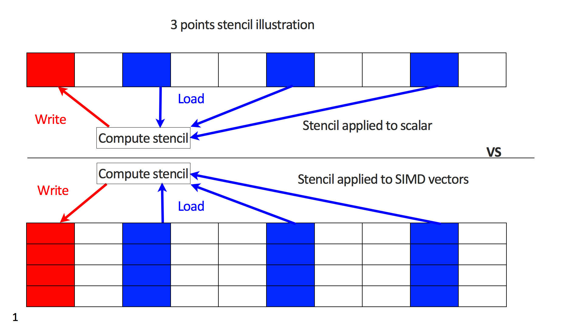
To address the performance issues with stencils, polyhedral programming methods such as tiling (Kamil et al., 2006) have been developed to reduce the number of cache misses in practise. However, while these methods can increase the codes performance, they can be highly invasive and do not fundamentally change the OI of the computational kernel. What we propose here is rather than computing the solution for a single shot per compute node, we instead compute the solution for multiple shots simultaneously, whereby the multiple solutions are stored continuously at the grid points. By choosing an appropriate number of shots this modification changes the computational kernel from being a stencil acting on scalar values to being a stencil acting on SIMD vectors.

While this approach is straightforward to implement, we show that we can readily double the performance of the solver. In this case study, we used the high-level programming language (MATLAB) interspersed with C functions that implement the time-stepping for multiple sources. OpenMP is used to parallelize the solver over space. The inner loop is over a fixed number of shots, therefore the compiler can readily vectorise it. The simplicity also makes it feasible to maintain adjoints and compute gradients and Jacobians according to the discretize-then-optimize method where the chain rule is applied to code . To illustrate this latter aspect, we first introduce our formulation for FWI, followed by a detailed discussion on our optimized implementation and its accuracy.

Scalar acoustic full-waveform inversion

For a spatially varying velocity model, \(c\), the acoustic wave equation in the time domain is given by: \[ \begin{equation} \frac{1}{c^2}\frac{\partial^2{u}}{\partial{t}^2} - \nabla^2 u = q, \label{AWE} \end{equation} \] where \(u\) is the wavefield, \(q\) is the source, \(\nabla\) is the Laplacian and \(\frac{\partial^2{u}}{\partial{t}^2}\) is the second-order time derivative. Given measurements of the pressure wavefield, the aim is to invert for the unknown velocity model, \(c\). Haber et al. (2012) shows that this can be expressed as the following PDE-constrained optimization problem: \[ \begin{equation} \begin{aligned} &\minim_{\vd{m},\vd{u}}\, \frac{1}{2}\norm{\vd{P}_r \vd{u} - \vd{d}}, \\ &\text{subject to} \ {A}(\vd{m})\vd{u} = \vd{q}_s, \end{aligned} \label{FWI} \end{equation} \] where \(\vd{P}_r\) is the projection operator onto the receiver locations, \(\vd{A(m)}\) is the discretized wave-equation matrix, \(\vd{m}\) is the set of model parameters (for this simple acoustic case \(\vd{m}:=1/c^2\)), \(\vd{u}\) is the discrete synthetic pressure wavefield, \(\vd{q}_s\) is the corresponding source and \(\vd{d}\) is the measured data. In this formulation, both \(\vd{u}\) and \(\vd{m}\) are the unknowns. We can rewrite Equation \(\ref{FWI}\) as a single objective function to be minimised (Virieux and Operto, 2009,Lions (1971)) , \[ \begin{equation} \minim_{\vd{m}} \Phi_s(\vd{m})=\frac{1}{2}\norm{\vd{P}_r {A}^{-1}(\vd{m})\vd{q}_s - \vd{d}}. \label{AS} \end{equation} \] To solve this optimization problem using a gradient-descent method we use the adjoint-state method to evaluate the gradient \(\nabla\Phi_s(\vd{m})\) (Plessix, 2006, Haber et al. (2012)): \[ \begin{equation} \nabla\Phi_s(\vd{m})=\sum_{t =1}^{n_t}\vd{u}[\vd{t}] \vd{v}_{tt}[\vd{t}] =\vd{J}^T\delta\vd{d}_s, \label{Gradient} \end{equation} \] where \(\delta\vd{d} = \left(\vd{P}_r \vd{u} - \vd{d} \right)\) is the data residual, and \(\vd{v}_{tt}\) is the second-order time derivative of the adjoint wave equation computed backwards in time: \[ \begin{equation} {A}^*(\vd{m}) \vd{v} = \vd{P}_r^* \delta\vd{d}. \label{Adj} \end{equation} \] As we can see, the adjoint-state method requires a wave-equation solve for both the forward and adjoint wavefields (many more solves are required if checkpointing is also used). While this computational cost clearly motivates the interest in optimizing the performance of the solvers, the importance of an accurate and consistent adjoint model in the solution of the optimisation problem motivates the requirement to keep the implementation relatively simple.

From matrix-vector to matrix-matrix products

For multiple RHSs, we can rewrite the wave equation as \[ \begin{equation} {A}(\vd{m})\vd{U} = \vd{Q}, \label{FwM} \end{equation} \] where \(\vd{U}\) is now a matrix with one wavefield for each source per column with the corresponding source located in the same column in \(\vd{Q}\). Since the same recasting applies to the adjoint (as long as the adjoint stencil is properly derived), we will only consider Equation \(\ref{FwM}\). This is implemented by arranging the wavefield matrix \(\vd{U}\) as a flat \(n_{RHS} \times N\) matrix while making sure that every column is memory aligned and contiguous so the compiler can readily vectorize the code. Figure 1 illustrates that the stencil kernel now operates on SIMD vectors rather than scalar values, thereby increasing the AI. This approach can be easily implemented for arbitrary time-stepping codes by adding an additional inner loop, which applies the stencil to a SIMD vector instead of a single scalar for each time step.

Swap free time-stepping with asynchronous I/O

Our implementation requires three consecutive wavefields (for the second time derivative in the gradient) and the next time step is computed from the current and previous time step.In order to propagate in time, the wavefields need to be swapped at the end of each time step so that the next time step becomes the current and the current the previous (see Algorithm 1). This can be accomplished in pure C implementation by a simple pointer swap at the end of each time step. However, moving pointers around] corrupts MATLAB’s memory management as it will not be aware of these swaps. We address this problem by working in cycles of three time steps as shown in Algorithm 1 and returning to MATLAB to perform the data swaps.In addition to these swaps, controlling the storage of the wavefield’s time history is another challenge. Computing multiple wavefields at once uses significantly more memory and increases the need for caching the time history to disk. Typically we save the time history of the forward modelled wavefields for all sources to disk every few time steps (4 to 8 or more in case the time is subsampled as recently proposed by Louboutin and Herrmann (2015)). However, the I/O overhead can be hidden within the compute cost by writing this data out to disk asynchronously. After combining these different steps, we arrive at the following workflow where every \(\vd{u}_i\) or \(\vd{v}_i\) are matrices of size \(n_{RHS} * N\):

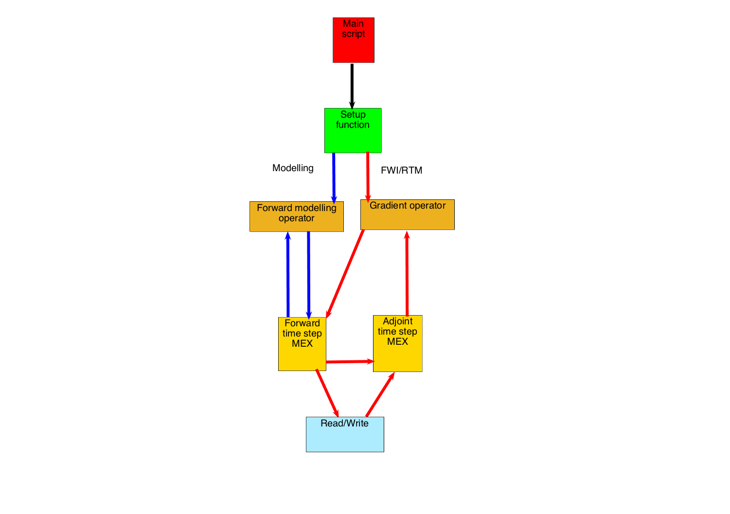
We can see from this algorithm that the wavefields are never swapped in the optimized low-level part implemented in C. In addition, the matrix \(\vd{u}_1\) is never updated allowing us to write it onto disk properly during the propagation. The pseudo-code for the adjoint modelling is similar. The full setup can be summarized by the following graphic and all calculations are done in single precision.

Computational efficiency

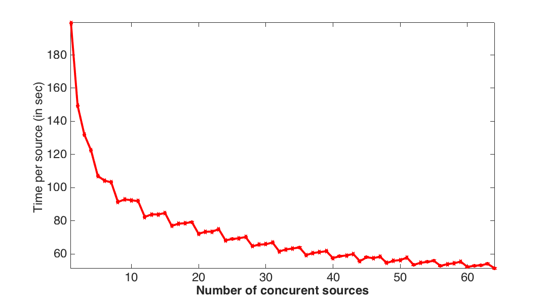
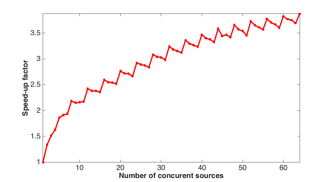
To evaluate the performance of our implementation, we start by measuring the relative speed up compared to modelings of one single right-hand-side (matrix-vector product) of our implementation designed to work with multiple RHSs vectorized (matrix-matrix products). For this purpose, we use a \(10\,\mathrm{Hz}\) Ricker wavelet as a source (same source time signature for all source positions), which generates \(4\,\mathrm{s}\) of . The velocity model is a two layer cube of size \(4.75\,\mathrm{km}\) discretized with a \(19\,\mathrm{m}\) grid in every direction (\(250^3\) grid points). We simulate \(1\) to \(64\) sources concurrently and we compare these times with the computation time per individual source by dividing the simulation time for the concurrent simulations by the number of concurrently computed sources. The timings and speed-up factors are shown on Figure 3. We can see from this figure that we obtained a speedup of a factor of \(3.8\) between operating on a single source and \(64\) sources. Even for \(20\) concurrent sources, we already have a speedup by \(2.5\). Because our vectors are aligned on \(32\) bits and we have to load two vectors at once, we observe a staircase behaviours where the performance increases every four sources.

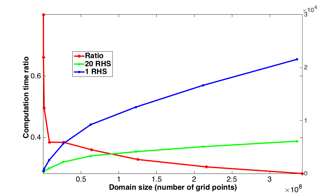
Now that we know that our method scales with the number of RHSs for a fixed domain size, we ensure this behaviour scales with the size of the model. For this purpose, we fix the number of RHSs to \(20\) as this number already gives a significant speedup. This choice also allows us to go to relatively large models given our memory of \(256\,\mathrm{GB}\) of RAM. For a fixed source and receiver setup, we increase the model size from \(20^3\) to \(700^3\) including an absorbing boundary layer of \(40\) grid points. The effective computational domain ranges from \(100^3\) to \(780^3\) grid points (\(2\,\mathrm{km}\) cube to \(15\,\mathrm{km}\) cube with a \(19\,\mathrm{m}\) grid at \(10\,\mathrm{Hz}\)). The results are presented in Figure 4, which shows the simulation times for \(4\,\mathrm{s}\) recordings of 3D shots as the model size increases. From this figure, we observe that the computational times for our multiple RHS approach grow moderately fast as a function of the model size compared to simulations of the wave equation on a shot-to-shot basis.

Gradient test

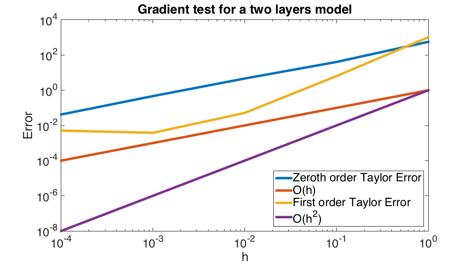
We know insure the accuracy of our operators from the FWI point of view. In order to have a correct update direction, we check that the gradient obtained satisfy the behaviour defined by the Taylor expansion of the FWI objective. This Taylor expansion also gives conditions on the forward modelling we require for an accurate modelling kernel. Mathematically, this conditions are expressed by \[ \begin{equation} \begin{aligned} &\Phi_s(\vd{m} + h \vd{dm}) = \Phi_s(\vd{m}) + \mathcal{O} (h) \\ &\Phi_s(\vd{m} + h \vd{dm}) = \Phi_s(\vd{m}) + h (\vd{J}[\vd{m}]^T\delta\vd{d})\vd{dm} + \mathcal{O} (h^2) \end{aligned} \label{GrFWI} \end{equation} \] meaning that the forward operator behave linearly with the model perturbation and that the Jacobian operator is a second-order operator. We can see on Figure 5 that our forward operator is exact for a broad range of perturbation and that our gradient stays accurate up til \(h\simeq10^{-2},10^{-3}\) corresponding to \(h^2\simeq10^{-4}.10^{-6}\). We therefore have operators accurate roughly up to single precision as expected.

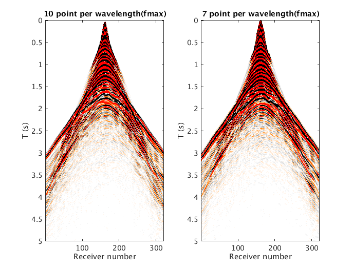
Finally we compared our implementation with an industrial solver. The implementation we use as a reference is a 3D SSE implementation (all written in intrinsic) with optimal tilling. It uses a 4th order in time method (against second order for us) with 10th order in space discretization (against 4th order) of the Laplacian allowing to work on grids 25% coarser than ours with larger time steps for a given physical domain and source peak frequency. We compare it for a model of size \(15\,\mathrm{km}\) by \(15\,\mathrm{km}\) with a \(2\,\mathrm{km}\) depth and \(10\,\mathrm{s}\) recording with a \(10\,\mathrm{Hz}\) Ricker wavelet. We will make a more rigorous comparison once more complex wave equations are included in our solver. For this setup the industrial solver took between 3 and 4 minutes to solve a single source with \(20\) thread and scales linearly with the number of threads. More explicitly \(20\) sources are solved in roughly \(1.5\,\mathrm{h}\) whether you solve each one a single thread in parallel or sequentially with the \(20\) threads dedicated to a single experiment. Our implementation took \(13\,\mathrm{h}\) with a fine grid (\(10\) grid points per wavelength) and \(3.5\,\mathrm{h}\) with a coarser one (\(7\) points per wavelength) for the \(20\) sources. A slice of the shot record on Figure 6 shows that our modelling generates a non-dispersive shot record even with only \(7\) points per wavelength. We show the shot record obtained on Figure 6.

Conclusions

The balance between productivity and performance is a key concern in rapidly evolving fields such as FWI. This is even more pronounced for any gradient based inversion problem where both the forward model and adjoint model have to be developed. In this work we took a first principles look at both a performance model for the underlying numerical method, namely the roofline model, and considered this in the specific context of FWI where shots are typically processed using task parallelism. We were readily able to double the speed of the code by redesigning the computational kernel so that its operational intensity was increased by processing multiple shots at once. This directly alleviates the key performance barrier for this problem, making the solver both less memory bounded and highly vectorized. The changes required to the source code were minimal and did not require any platform specific tuning whatsoever. While this work only considered the acoustic wave equation, the method has broad applicability and will have even greater impact as the number of parameters being inverted for increases as this will further increase the OI.

Acknowledgements

This work was financially supported in part by the Natural Sciences and Engineering Research Council of Canada Collaborative Research and Development Grant DNOISE II (CDRP J 375142-08) and the Imperial College London Intel Parallel Computing Centre. This research was carried out as part of the SINBAD II project with the support of the member organizations of the SINBAD Consortium.