Overview on anisotropic modeling and inversion

Philipp Witte^*, Mathias Louboutin and Felix J. Herrmann
Seismic Laboratory for Imaging and Modeling (SLIM), University of British Columbia

Summary:

This note provides an overview on strategies for modeling and inversion with the anisotropic wave equation. Since linear and non-linear inversion methods like least squares RTM and Full Waveform Inversion depend on matching observed field data with synthetically modeled data, accounting for anisotropy effects is necessary in order to accurately match waveforms at long offsets and propagation times. In this note, the two main strategies for anisotropic modeling by solving either a pseudo-acoustic wave equation or a pure quasi-P-wave equation are discussed and an inversion workflow using the pure quasi-P-wave equation is provided. In particular, we derive the exact adjoint of the anisotropic forward modeling and Jacobian operator and give a detailed description of their implementation. The anisotropic FWI workflow is tested on a synthetic data example.

Introduction

Seismic imaging and inversion of large scale data sets require an accurate and efficient modeling kernel for numerically solving the wave equation. Especially for seismic field data with large offsets, the acoustic approximation of wave propagation is no longer appropriate to accurately match the waveforms of the observed data, since travel times and amplitudes are influenced by anisotropy effects. In exploration seismology, these effects are mostly related to the fact that a wave that travels through several layers of (isotropic) rocks, at which the layer thickness is much smaller than the dominant wavelength, behaves like a wave propagating through a homogeneous but anisotropic medium. For this reason, anisotropy in sedimentary settings is primarily observed in the vertical direction and can be approximated by vertical transverse isotropic (VTI) or tilted transverse isotropic (TTI) models. Because the effects of anisotropy in sedimentary layers are usually also small (no more than 10-20 percent), a weak anisotropy approximation has been derived at which the effects of anisotropy are described by the Thomsen parameters \(\epsilon\) and \(\delta\) (Thomsen, 1986)

Derived from the dispersion relation in terms of the Thomsen parameters, Alkhalifah (2000) introduced a pseudo-acoustic wave equation to describe wave propagation in transverse isotropic media such as VTI and TTI with forth order partial derivatives in space and time. Based on this equation, mainly two different approaches for modeling VTI and TTI wave equations have evolved. The first equation that is commonly used in the literature for seismic imaging (RTM) is a pseudo-acoustic wave equation, expressed as a coupled 2 by 2 system of equations with a pseudo-pressure field P and an auxiliary field Q. This approach is followed for example by Zhang et al. from CGG (2011). The alternative approach is a purely quasi-P wave equation that completely decouples the pressure wavefield from the full elastic wavefield. Modeling and imaging workflows based on this equation have been developed by Chu et al. from Conoco Philips (2011), Xu and Zhou from Statoil (2014), Zhan et al. (2013) and Zhang et al. (2005). The main advantage of the pure P-wave equation is that is is completely free of S-wave artifacts and is computationally less expansive and more memory efficient, since the pseudo-acoustic wave equation requires the computation and (possibly) the storage of two wavefields. Also, the pure P-wave equation is numerically more stable for strongly varying angles in TTI media (Zhan et al., 2013), since the presence of S-wave artifacts decreases the stability of the pseudo-acoustic wave equation. On the other hand, the pseudo-acoustic equation can be solved with both finite difference (FD) as well as pseudo spectral (PS) methods, whereas the pure P-wave equation requires the high accuracy of PS operators, making this approach computationally expensive, as each time step involves a large number of forward and inverse FFTs.

For incorporating anisotropy in the time-domain modeling kernel of the SLIM inversion workflow, we use the pure quasi-P-wave equation in the time-spacenumber domain as derived by Zhang et al. (2005) or Chu et al. (2011). Their discretized TTI wave equation is second order in time and uses the PS method for the Laplacian operator. The main advantage of this formulation is that the anisotropy parameters only appear in the expression for the Laplacian, which allows us to use our functions for forward modeling and back propagation, as well as the application of forward and adjoint Jacobians from our existing workflow by simply replacing the Laplacian operator.

Isotropic modeling and inversion in the time domain

Since the anisotropic modeling and inversion workflow is completely based on our isotropic implementation, we first outline the discretization for the isotropic acoustic wave equation and then derive the anisotropic Laplacian operator based on the TTI equation of Zhang et al (2005). Our existing workflow is then easily extended to anisotropy by swapping out the Laplacian operator.

The isotropic acoustic wave equation in continuous form is given by \[ \begin{equation} m \frac{\partial^2{u}}{\partial{t}^2} - \nabla^2 u = q \label{AWE} \end{equation} \] where \(m\) is the (spatially varying) squared slowness, \(u\) is the pressure wave field and \(q\) is the source term. We discretized this equation using a second order leap frog scheme for the time derivative \[ \begin{equation} \frac{\partial^2 u}{\partial t ^2} (t) \approx \frac{\mathbf{u}^{k+1} -2 \mathbf{u}^k + \mathbf{u}^{k-1}}{\delta t^2} \label{Eul} \end{equation} \] and a finite difference star stencil for the spatial derivative. Along one dimension, the second order Laplacian operator is given by \[ \begin{equation} \frac{\partial^2 u}{\partial x ^2} \approx \frac{1}{h^2}\sum_{i=-\frac{p}{2}}^{\frac{p}{2}} \alpha_i \mathbf{u}_i = \mathbf{D_{xx}} \label{Dx} \end{equation} \] where \(p\) is the space discretization order and \(\alpha_i\) are the coefficients of the FD stencil. Using Kronecker products, the operator can be extended to act on a three-dimensional space of dimensions \(N_x\) x \(N_y\) x \(N_z\): \[ \begin{equation} \mathbf{L_x}= \mathbf{D_{xx}} \otimes \mathbf{I_{yy}} \otimes \mathbf{I_{zz}} \label{Lx} \end{equation} \] The three-dimensional Laplacian is then given as the sum of the 1D Laplacians in each direction \(\mathbf{L}=\mathbf{L_x + L_y +L_z}\) . Finally, we write the fully discretized acoustic wave equation as \[ \begin{equation} \mathbf{A_1 u^{k+1}}+\mathbf{A_2 u^k} + \mathbf{A_3 u^{k-1}}=\mathbf{q^{k+1}} \label{TS} \end{equation} \] where \(\mathbf{q^k}\) is the source term at time step \(k\) and the matrices are define as \[ \begin{equation} \begin{aligned} \mathbf{A_1} &=\mathbf{diag}(\frac{\mathbf{m}}{\triangle t^2}) \\ \mathbf{A_3} &=\mathbf{diag}(\frac{\mathbf{m}}{\triangle t^2}) \\ \mathbf{A_2} &=-\mathbf{L}-2\mathbf{diag}(\frac{\mathbf{m}}{\triangle t^2}) \end{aligned} \label{A123} \end{equation} \] One time step of either the forward wavefield \(\mathbf{u}\) or the adjoint wavefield \(\mathbf{v}\) is calculated by \[ \begin{equation} \mathbf{u}^\mathbf{k+1} = \mathbf{A_1}^{-1} (-\mathbf{A_2 u^{k}} - \mathbf{A_3 u^{k-1}}+\mathbf{q^{k+1}}) \label{TS1} \end{equation} \] and \[ \begin{equation} \mathbf{v}^\mathbf{k-1} = \mathbf{A_3}^{-T} (-\mathbf{A_2}^T \mathbf{v^{k}} - \mathbf{A_1}^T \mathbf{v^{k+1}}+\mathbf{\delta d}) \label{TSA} \end{equation} \] respectively, at which \(\delta \mathbf{d}\) is the adjoint source.

For calculating an RTM image or gradient updates of the FWI objective function, we furthermore require the action of the (adjoint) Jacobian of the forward modeling operator. Writing Equation \(\ref{TS}\) as one large system of equations, denoting the modeling matrix as a nonlinear operator \(\mathcal{A}(\mathbf{m})\) and taking the partial derivative with respect to the model parameter yields \[ \begin{equation} \frac{\partial}{\partial \mathbf{m}} \Big( \mathcal{A}(\mathbf{m})\mathbf{u=\mathbf{q}}\Big) \iff \frac{\partial \mathcal{A}(\mathbf{m})}{\partial \mathbf{m}} \mathbf{u} + \mathcal{A}(\mathbf{m}) \frac{\partial \mathbf{u}}{\partial \mathbf{m}} = 0 \label{Eq1} \end{equation} \] which gives us the expression for the Jacobian and its adjoint \[ \begin{equation} \mathbf{J} = \frac{\partial \mathbf{u}}{\partial \mathbf{m}} = - \mathcal{A}(\mathbf{m})^{-1} \Big( \frac{\partial \mathcal{A}(\mathbf{m})}{\partial \mathbf{m}} \mathbf{u} \Big) \label{Eq3} \end{equation} \] \[ \begin{equation} \mathbf{J}^T = - \Big( \frac{\partial \mathcal{A}(\mathbf{m})}{\partial \mathbf{m}} \mathbf{u} \Big)^T \mathcal{A}(\mathbf{m})^{-T} \label{Eq4} \end{equation} \] and the action of the adjoint Jacobian on the vector \(\delta \mathbf{m}\), which corresponds to the gradient of the FWI least squares objective function: \[ \begin{equation} \mathbf{J}^T \delta \mathbf{m} = - \Big( \frac{\partial \mathcal{A}(\mathbf{m})}{\partial \mathbf{m}} \mathbf{u} \Big)^T \mathcal{A}(\mathbf{m})^{-T} \delta \mathbf{d} \label{Eq5} \end{equation} \] where the second part of this equation is the solution of the adjoint wave equation given by Equation \(\ref{TSA}\) . The derivative of \(\mathcal{A}(\mathbf{m})\) with respect to \(\mathbf{m}\) is just the temporal derivative of the forward wavefield \(\mathbf{u}\). Calculating the gradient of the FWI objective in the time stepping manner is therefore done by

1. Modeling the forward wavefield \(\mathbf{u}\) for all time steps \(k=1,...,nt\) and storing the wavefields (Equation \(\ref{TS1}\))
2. Modeling the adjoint wavefield \(\mathbf{v}\) in reverse order \(k=nt,...,1\) (Equation \(\ref{TSA}\)) and multiplying the adjoint wavefields of each time step with \(\frac{1}{\Delta t^2}\) (for \(\mathbf{v^{k+1}}\) and \(\mathbf{v^{k-1}}\)) or \(\frac{-2}{\Delta t^2}\) (for \(\mathbf{v^{k}}\)). This corresponds to applying a time derivative operator \(\mathbf{D}\) to the wavefield.
3. Multiplying the wavefields and updating the gradient within the reverse time loop: \(g = g - (\mathbf{u^{k-1}})^T\mathbf{diag(D v^{k-1})}\)

Extension to anisotropy

For the incorporation of anisotropy we start from the two-dimensional pure P-wave-equation for TTI media with weak anisotropy by Zhan et al. (2005): \[ \begin{equation} \begin{aligned} m\frac{\partial^2 U(k_x,k_z,t)}{\partial t^2} = \Big[ k_x^2+k_z^2 + &(2\delta \sin^2{\theta} \cos^2{\theta} + 2\epsilon \cos^4{\theta}) \frac{k_x^4}{k_x^2+k_z^2}+ \\ & (2\delta \sin^2{\theta} \cos^2{\theta} + 2\epsilon \sin^4{\theta}) \frac{k_z^4}{k_x^2+k_z^2}+ \\ & (-\delta \sin^2{2\theta} + 3\epsilon \sin^2{2\theta} + 2\delta \cos^2{2\theta}) \frac{k_x^2 k_z^2}{k_x^2+k_z^2}+ \\ & (\delta \sin{4\theta} - 4\epsilon \sin{2\theta}\cos^2{\theta} ) \frac{k_x^3 k_z}{k_x^2+k_z^2} + \\ & (-\delta \sin{4\theta} - 4\epsilon \sin{2\theta}\sin^2{\theta} ) \frac{k_x k_z^3}{k_x^2+k_z^2} \Big] U(k_x,k_z,t) \end{aligned} \label{we1} \end{equation} \] \(U\) is the wavefield in the time-wavenumber domain and \(k_x\) and \(k_z\) are the spatial wave numbers in \(x\) and \(z\) direction respectively. \(\epsilon\) and \(\delta\) are the Thomsen parameters and \(\theta\) is the angle of the symmetry axis measured against the vertical direction and for \(\theta=0\) the equation reduces to the VTI equation. Using a second order leap frog scheme in time and including the source term \(q\), this equation can be written as \[ \begin{equation} \mathbf{diag}(\frac{\mathbf{m}}{\Delta t^2}) \Big( \mathbf{u}^{n+1} -2 \mathbf{u}^n + \mathbf{u}^{n-1} \Big) - \mathbf{L} \mathbf{u}^n = \mathbf{q}^{n+1} \label{we2} \end{equation} \] which corresponds exactly to Equations \(\ref{TS}\) and \(\ref{A123}\), only that the Laplacian is now given by: \[ \begin{equation} \mathbf{L} = \text{real}\Big( \textbf{F}^* \text{diag}(\textbf{k}_{ani}) \textbf{F} \Big) \label{laplace} \end{equation} \] \(\textbf{L}\) is a matrix free operator that can be transposed in order to calculate the backprogagated wavefield. \(\textbf{F}\) represents the matrix for the (multidimensional) Fourier transformation and \(\textbf{k}_{ani}\) is the term within the square brackets in Equation \(\ref{we1}\) that contains the (spatially varying) anisotropy parameters. The pseudo-code for building the Laplacian is given in the appendix. In our anisotropic workflow we still want to invert for the squared slowness only, but we want to use the TTI wave equation for the forward and back propagations. Because the Laplacian is independent of the slowness, differentiating the modeling operator with respect to \(\mathbf{m}\) does not change the expression for the adjoint Jacobian (Equation \(\ref{Eq5}\)). Therefore we can obtain the true Jacobian and it’s adjoint of the anisotropic Modeling operator by using the same code as before by just swapping the operator for the Laplacian.

Data example

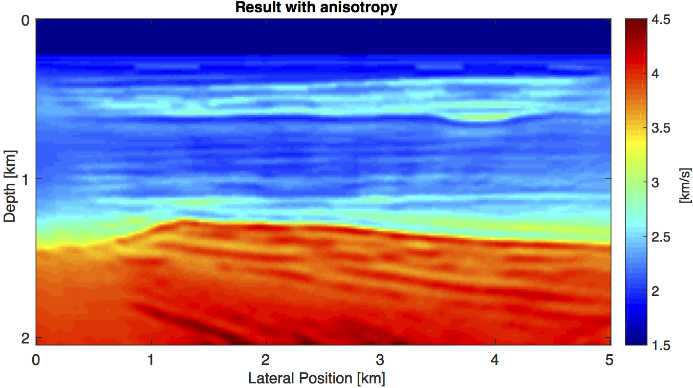
We test the anisotropic FWI workflow by inverting the two-dimensional BG velocity model. We generate observed data with anisotropy effects using an epsilon and a delta model, as well as a tilt angle that is derived from the velocity model (Figure 2). We then perform two FWI runs of 30 iterations each, both starting from the same initial model. In the first run, the (anisotropic) data is inverted with the isotropic engine, i.e. the Thomsen parameters are set to zero, whereas in the second run, we invert with the true model for the Thomsen parameters.

Alternative derivative operators

The main problems in our current implementation are numerical stability and computational efficiency. Experiments with the modeling kernel show that sharp and large contrasts within the models of the anisotropy parameters cause artifacts in wavefields. More importantly, using pseudo-spectral methods for the spatial derivative requires a forward and inverse Fourier transform of the entire wavefield at each time step, which becomes especially problematic in 3D FWI. For these reasons, we are investigating in alternatives for the derivative matrices, as the Eigen-decomposition Pseudo-Spectral (EPS) method (K. Sandberg and Wojciechowski, 2011) which is based on integral operators with a kernel function \(K(x,y)\) \[ \begin{equation} Lf(x) =\int_a^b K(x,y)f(y)dy \label{epsop} \end{equation} \] where \(K(x,y)\) is constructed from a set of orthonormal functions \(\{u_m\}_{m=1}^{\infty}, \{v_m\}_{m=1}^{\infty}\) and constants \(\lambda_m\): \[ \begin{equation} K(x,y) = \sum_{m=1}^\infty \lambda_m u_m(x)v_m(y) \label{kernel} \end{equation} \] To construct the discrete operator, the sum of the Kernel function is truncated after \(N_c\) terms and the integral is replaced by quadratures on nodes \(\{\theta_k\}_{k=1}^N\) with weights \(\{w_k\}_{k=1}^N\): \[ \begin{equation} Lf(\theta_k) = \sum_{m=1}^{N_c} \lambda_m u_m(\theta_k) \sum_{l=1}^{N} w_l v_m(\theta_l) f(\theta_l) \label{discreteDerv} \end{equation} \] Possibilities for the quadratures are Gauss-Legendre quadratures or prolate spherical wave functions (PSWFs), which have been shown to allow exact numerical integration of band limited function on an interval (Beylkin and Sandberg, 2005). The derivative Matrix itself is given by \[ \begin{equation} L_{kl} = \sum_{m=1}^{N_c} \lambda_mu_m(\theta_k)w_lv_m(\theta_l) \label{discreteL} \end{equation} \] Due to the truncation of the Kernel sum, the resulting operator has a small matrix norm, allowing larger time steps and an optimal spatial sampling rate close to two grid points per wavelength. However, the truncated elements are responsible for absorbing high frequency oscillations, which is highly desirable for wave propagation in which the functions are typically not truly band limited (Sandberg et. al, 2011). A full rank operator which still has a small matrix norm, can be constructed by adding a tail to the operator \[ \begin{equation} L_{kl} = \sum_{m=1}^{N_c} \lambda_m u_m(\theta_k)w_l v_m(\theta_l) + \sum_{m=N_c + 1}^{N} \lambda_m \tilde{u}_m(\theta_k)w_l \tilde{v}_m(\theta_l) \label{discreteFull} \end{equation} \] where \(\{\tilde{u}_m(\theta_l)\}_{m=N_c+1}^{N}\) are the last \(N-N_c\) vectors that have been orthogonalized with respect to the inner product \[ \begin{equation} \langle u_m(\theta_l), u_n(\theta_l)\rangle = \sum^{N}_{l=1} w_l u_m(\theta_l) u_n(\theta_l) \label{inProc} \end{equation} \] The second derivative operator \(D^2\) of rank \(N\) with Dirichlet boundary conditions can be constructed from its eigen decomposition \[ \begin{equation} \Big\{-\frac{m^2\pi^2}{4},\sin\Big( \frac{m\pi}{2}(x+1)\Big)\Big\}_{m=1}^N \label{SVDlaplace} \end{equation} \] The rank completed operator is then given by \[ \begin{equation} \begin{aligned} D^2_{kl} = -\frac{\pi^2}{4} \Bigg( \sum_{m=1}^{N_c} m^2 \sin\Big( \frac{m\pi}{2}(\theta_k+1)\Big) w_l \sin\Big( \frac{m\pi}{2}(\theta_l+1)\Big) &+ \\ \sum_{m=N_c+1}^{N} m^2\tilde{u}_m(\theta_k) w_l \tilde{v}_m(\theta_l) &\Bigg) \end{aligned} \label{Lcomplete} \end{equation} \] The one-dimensional second derivative operator can be used to construct the 2D Laplacian in the same way as before by using Kronecker products. The advantage of the EPS derivative operator is its high accuracy in the range of machine precision, as well as allowing close to optimal sampling in space and time. However, the 1D operator itself is a dense matrix and in order to allow fast matrix vector multiplications needs to be represented in e.g. the partitioned low rank (PLR) or hierarchical semi-separable (HSS) format. Whether the EPS method can be extended to anisotropy and is computationally more efficient in this context than the PS method, is currently under investigation.

Outlook: 3D Extension

Extension of the described method to 3D is straight forward. The isotropic modeling and inversion workflow itself is already implemented for 3D, therefore only the 3D anisotropic Laplacian needs to be added. The operator is constructed in the same manner as before, only that \(\mathbf{F}\) now is the 3D discrete Fourier transform and the central term \(diag (\mathbf{k}_{ani})\) is constructed from the 3D pure P-wave equation, which is given in Chu et al. (2011).

Appendix

The following algorithm shows construction of the anisotropic Laplacian operator (Equation \(\ref{laplace}\)). We use the SPOT toolbox (http://www.cs.ubc.ca/labs/scl/spot/) which allows us to represent the Fourier transform as matrix free operators. This means the 2D Fourier operator \(\mathbf{F}\) is never explicitly formed, but can be used like a matrix, i.e. it can be transposed or applied to a vector. Furthermore, SPOT operators can be combined to perform multiple operations consecutively. This is used for the Laplacian operator, whose application on a vector consists of a forward Fourier transform, multiplication with the diagonal matrix containing the anisotropy parameters (\(\mathbf{k}_{ani}\)) and the inverse Fourier transform. The (matrix-free) operator \(\mathbf{L}\) can be transposed as well in order to calculate the adjoint wavefields (Equation \(\ref{TSA}\)).

% 1D wavenumbers (row vectors)
\(\mathbf{k}_z = \frac{2\pi}{bz-az}*[0:(\frac{nz}{2}-1), 0,(-\frac{nz}{2}+1):-1]\)
\(\mathbf{k}_x = \frac{2\pi}{bx-ax}*[0:(\frac{nx}{2}-1), 0,(-\frac{nx}{2}+1):-1]\)

% Construct 2D wavenumber field from 1D vectors
\(\mathbf{K}_z = \mathbf{e}_{nx} \otimes \mathbf{k}_z^T\) % \(\mathbf{e}\) denotes an all ones row vector of length \(nx\)
\(\mathbf{K}_x = \mathbf{e}_{nz}^T \otimes \mathbf{k}_x\)

% Mixed wavenumber fields by entrywise products (\(\odot\)), division ( ./ ) and exponantiation
\(\mathbf{K}_{1} = \mathbf{K}_x^4 \text{ ./ } (\mathbf{K}_x^2 + \mathbf{K}_z^2) \)
\(\mathbf{K}_{2} = \mathbf{K}_z^4 \text{ ./ } (\mathbf{K}_x^2 + \mathbf{K}_z^2) \)
\(\mathbf{K}_{3} = \mathbf{K}_x^2 \odot \mathbf{K}_z^2 \text{ ./ } (\mathbf{K}_x^2 + \mathbf{K}_z^2) \)
\(\mathbf{K}_{4} = \mathbf{K}_x^3 \odot \mathbf{K}_z \text{ ./ } (\mathbf{K}_x^2 + \mathbf{K}_z^2) \)
\(\mathbf{K}_{5} = \mathbf{K}_x \odot \mathbf{K}_z^3 \text{ ./ } (\mathbf{K}_x^2 + \mathbf{K}_z^2) \)

% 2D gridded Thomsen parameters in tilted medium
\(\mathbf{T}_1 = 2 \delta \odot \sin^2{\theta} \odot \cos^4{\theta} + 2\epsilon \odot \cos^4{\theta}\)
\(\mathbf{T}_2 = \mathbf{T}_1\)
\(\mathbf{T}_3 = -\delta \odot \sin^2{2\theta} + 3\epsilon \odot \sin^2{2\theta} + 2\delta \odot \cos^2{2\theta}\)
\(\mathbf{T}_4 = \delta \odot \sin{4\theta} - 4\epsilon \odot \sin{2\theta} \odot \cos^2{\theta}\)
\(\mathbf{T}_5 = -\delta \odot \sin{4\theta} - 4\epsilon \odot \sin{2\theta} \odot \sin^2{\theta}\)

% Combine all terms and vectorize
\(\mathbf{k}_{ani} = \text{vec} \big( -\mathbf{K}_x^2 - \mathbf{K}_z^2 + \mathbf{T}_1 \odot \mathbf{K}_1 + \mathbf{T}_2 \odot \mathbf{K}_2 + \mathbf{T}_3 \odot \mathbf{K}_3 + \mathbf{T}_4 \odot \mathbf{K}_4 + \mathbf{T}_5 \odot \mathbf{K}_5 \big)\)

% 2D Fourier transform
\(\mathbf{F} = (\mathbf{I}_{nx} \otimes \mathbf{F}_z) \cdot (\mathbf{F}_x \otimes \mathbf{I}_{nz})\)  % where \(\mathbf{I}_x\) is the Identity matrix and \(\mathbf{F}_x\) is the 1D Fourier matrix of the respective dimension.

% Laplacian operator
\(\mathbf{L} = \text{real} \Big( \mathbf{F}^* \text{diag} (\mathbf{k}_{ani}) \mathbf{F} \Big)\)   % where \(^*\) is the conjugate transpose

Acknowledgements

This work was in part financially supported by the Natural Sciences and Engineering Research Council of Canada Discovery Grant (22R81254) and the Collaborative Research and Development Grant DNOISE II (375142-08). This research was carried out as part of the SINBAD II project with support from the following organizations: BG Group, BGP, CGG, Chevron, ConocoPhillips, Petrobras, PGS, WesternGeco, and Woodside.