Regularizing waveform inversion by projections onto convex sets — application to the 2D Chevron 2014 synthetic blind-test dataset

Introduction

Full-waveform inversion (FWI) involves solving a nonlinear optimization problem and it is an inverse problem which may require some form of regularization to yield solutions which conform with our knowledge about the Earth at the survey location. In this expanded abstract we propose a regularization strategy based on solving constrained problems by projection onto intersections of convex sets. We incorporate multiple pieces of prior information about the Earth into the FWI optimization scheme, in an approach similar to Baumstein (2013). This avoids the use of quadratic penalties. It is also shown how the constrained problem formulation incorporates several preexisting regularization ideas. Application of the method to the blind-test data by Chevron for the 2014 SEG conference illustrates the effectiveness of the proposed approach.

FWI with regularization by projection onto the intersection of convex sets

In search of a flexible and easy to use framework, which can incorporate most existing ideas in the geophysical community to regularize the waveform inversion problem, we propose to solve constrained optimization problems of the form \[ \begin{equation} \min_{\bm} f(\bm) \quad \text{s.t.} \quad \bm \in \mathcal{C}_1 \bigcap \mathcal{C}_2. \label{prob_constr} \end{equation} \] The model vector, \(\bm\) (often velocity), and the objective function can measure the difference between predicted data and observed data, \(f(\bm)=\frac{1}{2}\| P H(\bm)^{-1}\bq - \bd \|^2_2\) as is often used in FWI. \(H\) is the discretized Helmholtz equation, \(P\) restricts the wavefield to the receiver locations, \(\bq\) is the vector containing source function and location and \(\bd\) is the observed data. It is also possible to use other norms and objective functions, for example objective functions corresponding to the Wavefield Reconstruction Inversion (WRI, Leeuwen and Herrmann, 2013): \(f(\bm)=\frac{1}{2}\| P \bar{\bu} - \bd \|^2_2 +\frac{\lambda^2}{2}\| H(\bm) \bar{\bu} - \bq \|^2_2\) with \(\bar{\bu}=(\lambda^2 H^*H + P^*P)^{-1} (\lambda^2 H^*\bq + P^* \bd)\).

\(\mathcal{C}_1\) and \(\mathcal{C}_2\) are convex sets (more than 2 sets can be used). Intuitively, the line connecting any two points in a convex set is also in the set: for all \(x\),\(y\) \(\in \mathcal{C}\) the following holds: \(c x +(1-c)y \in \mathcal{C}\), \(0 \leq c \leq 1\). Each set represents a known piece of information about the Earth; a constraint which the estimated model has to satisfy. The model is required to be in the intersection of the two sets, denoted by \(\mathcal{C}_1 \bigcap \mathcal{C}_2\). The intersection of convex sets is also convex. To summarize, solving Problem \(\ref{prob_constr}\) means we try to minimize the data misfit while satisfying constraints, which represent the known information about the geology. Below are two useful convex sets which are also used in the examples. Bound-constraints can be defined element-wise as \[ \begin{equation} \mathcal{C}_1 \equiv \{ \bm \: | \: \bb_l \leq \bm \leq \bb_u \}. \label{cnx_set_def1} \end{equation} \] If a model is in this set, then every model parameter value is between a lower bound \(\bb_l\) and upper bound, \(\bb_u\). These bounds can vary per model parameter and can therefore incorporate spatially varying information about the bounds. Bound constraints can also incorporate a reference model by limiting the maximum deviation from this reference model as: \(\bb_l = \bm_{\text{ref}} - \delta\bm\). The projection onto \(\mathcal{C}_1\), denoted as \(\mathcal{P}_{\mathcal{C}_1}\), is the elementwise median: \(\mathcal{P}_{\mathcal{C}_1} (\bm)= \text{median}\{ \bb_l , \bm , \bb_u\}\).
The second convex set that is used here is a subset of the wavenumber domain representation of the model (spatial Fourier transformed). This convex set can be defined as \[ \begin{equation} \mathcal{C}_2 \equiv \{ \bm \: | \: E^*F^*(I-S)FE\bm=0\}. \label{cnx_set_def2} \end{equation} \] This set is defined by a series of matrix multiplications and means that we apply the mirror-extension operator, \(E\) to the model \(\bm\) to prevent wrap-around effects due to applying linear operations in the wavenumber domain. Next, the mirror extended model is spatially Fourier transformed using \(F\). In this domain we require the wavenumber content outside a certain range to be equal to zero. This is enforced by the diagonal (windowing) matrix \(S\). This represents information that the model should have a certain minimum smoothness. In case we expect an approximately horizontally layered medium without sharp contrasts, we can include this information by requiring the wavenumber content of the model to vanish outside of an elliptical zone around the zero wavenumber point (see also Brenders and Pratt (2007)). In other words, more smoothness in one direction is required than in the other direction. The adjoint of \(F\), (\(F^*\)) transforms back from the wavenumber to the physical domain and \(E^*\) goes from mirror-extended domain to the original model domain. The projection onto \(\mathcal{C}_2\), denoted as \(\mathcal{P}_{\mathcal{C}_2}\), is given by \(\mathcal{P}_{\mathcal{C}_2} (\bm)= E^*F^*SFE\bm\).

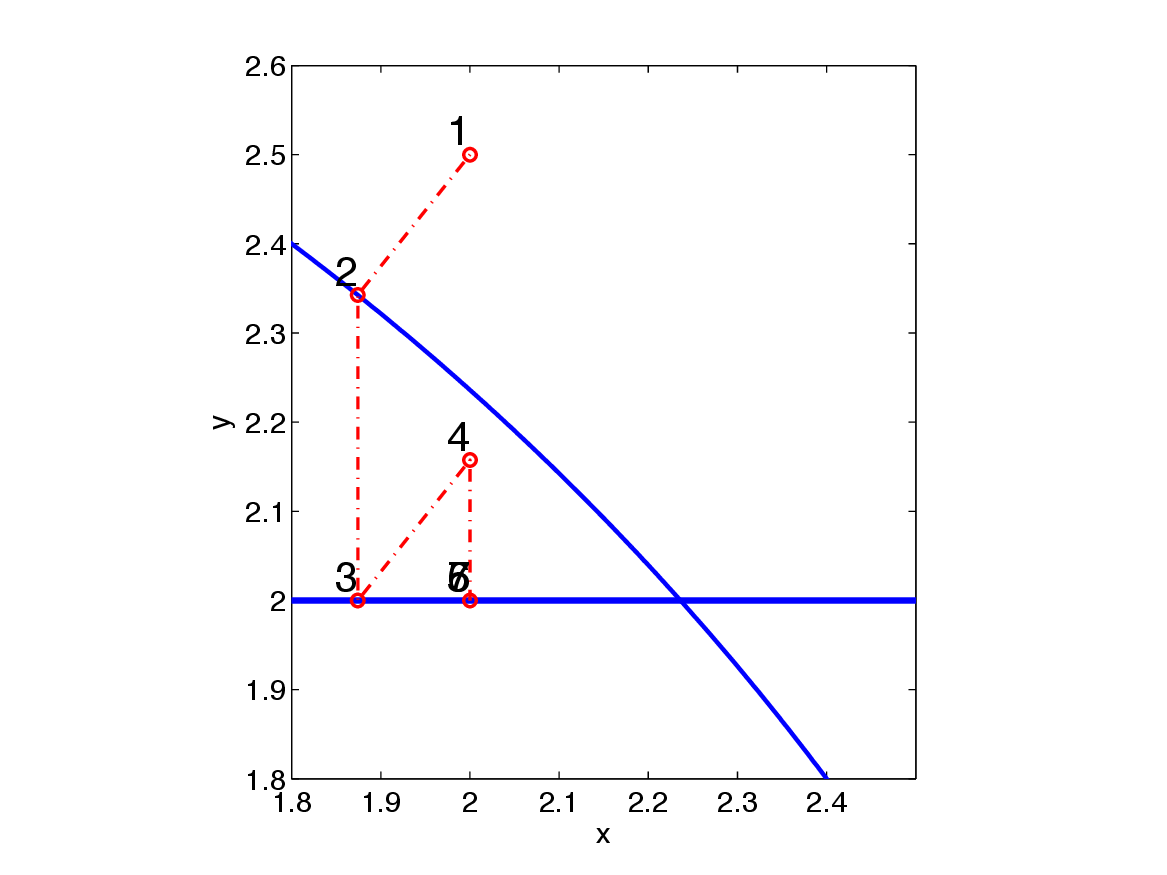
A basic way to solve Problem \(\ref{prob_constr}\) is to use the projected-gradient algorithm, which has the main step \(\bm_{k+1}=\mathcal{P}_{\mathcal{C}} (\bm_k - \gamma \nabla_{\bm}f(\bm))\), with a step length \(\gamma\). \(\mathcal{P}_{\mathcal{C}}=\mathcal{P}_{\mathcal{C}_1 \bigcap \mathcal{C}_2}\) is the projection onto the intersection of all convex sets the model is required to be in. “The projection onto” means we need to find the point that is in both sets and closest to the current proposed model estimate generated by \((\bm_k - \gamma \nabla_{\bm}f(\bm))\). To find such a point, defined mathematically as \[ \begin{equation} \mathcal{P_{C}}({\bm})=\arg \min_{\mathbf{x}} \| \mathbf{x}-\bm \|_2 \quad \text{s.t.} \quad \mathbf{x} \in \mathcal{C}_1 \bigcap \mathcal{C}_2, \label{def_proj} \end{equation} \] we can use a splitting method such as Dykstra’s projection algorithm (Bauschke and Borwein, 1994). This algorithm finds the projection onto the intersection of the two sets, by projecting onto each set separately. This is a cheap and simple algorithm and enables projections onto complicated intersections of sets. The algorithm is given by Algorithm 1.

While gradient-projections is a solid approach, it can also be relatively slowly converging. A potentially much faster algorithm is the class of projected Newton-type algorithms (PNT) (see for example Schmidt et al., 2012). Standard Newton-type methods iterate, \(\bm_{k+1}= \bm_k - \gamma B^{-1}\nabla_{\bm}f(\bm)\), with \(B\) an approximation of the Hessian. At every iteration, the PNT method finds the new model by solving the constrained quadratic problem \[ \begin{equation} \bm_{k+1}= \arg \min_{\bm \in \mathcal{C}_1 \bigcap \mathcal{C}_2} Q(\bm) \label{PNt_cquad_sub} \end{equation} \] where the local quadratic model is given by \(Q(\bm) = f(\bm_{k}) + (\bm - \bm_k)^* \nabla_{\bm}f(\bm_k) + (\bm - \bm_k)^* B_k (\bm - \bm_k)\). No additional Helmholtz problems need to be solved. This method does not simply project an update. The PNT algorithm needs the objective function value, its gradient, approximation to the Hessian and an algorithm to solve the constrained quadratic sub-problem (Problem \(\ref{PNt_cquad_sub}\)), which in turn needs an algorithm (Dykstra) to solve the projection problem (Problem \(\ref{def_proj}\)). The PNT sub-problem can be solved in many ways; we select the alternating direction method of multipliers (ADMM) algorithm, see for example Eckstein and Yao (2012). ADMM can solve Problem \(\ref{PNt_cquad_sub}\) very efficiently provided the approximate Hessian, \(B\), is easy to invert. The Hessian approximation is assumed to be diagonal or sparse-banded and a lot easier to invert than a discrete Helmholtz system. Examples of this type of Hessian approximation can be found in Shin et al. (2001) and Leeuwen and Herrmann (2013). The Dykstra-splitting algorithm solves a sub-problem inside the ADMM algorithm, which is also a splitting-algorithm.

PNT has a similar computational cost as the standard projected-Newton algorithm; the same number of Helmholtz systems need to be solved. The additional cost is low, because the projections are cheap to compute and the inversion of the Hessian matrix is assumed cheap by the assumptions listed above.

The final optimization algorithm is given by Algorithm 2 and can best be described as Dykstra’s algorithm within ADMM within a projected-Newton type method. At every iteration, the constraints are satisfied exactly.

Practical considerations

The above projected Newton-type of approach with convex constraints provides the formal optimization framework with which we will carry out our experiments. Before demonstrating the performance of our approach, we discuss a number of practical considerations to make the inversion successful.

Frequency continuation. We divide the frequency spectrum into overlapping frequency bands of increasing frequency. This multiscale continuation makes the approach more robust against cycle skips.

Selection of the smoothing parameter. Although there is no penalty parameter to select in our method, we do need to define the convex sets onto which we project. The minimum-smoothness constraints require two parameters; one which indicates how much smoothness is required and one which indicates the difference between horizontal and vertical smoothness. At the start of the first frequency batch, these parameters are chosen such that the minimum smoothness constraints correspond to the smoothness of the initial guess and we add some ‘room’ to update the model to less smooth model. This is the only user intervention of our regularization framework. Subsequent frequency batches multiply the selected parameters by the empirical formula \(d \frac{f_{\text{max}}}{v_\text{min}}\), where \(d\) is the grid-point spacing, \(f_{\text{max}}\) the maximum frequency of the current batch and \(v_\text{min}\) the minimum velocity in the current model. This automatically adjusts the selected parameters for changing grids, frequency and velocity.

Data fit for Wavefield Reconstruction Inversion. Our inversions are carried out with Wavefield Reconstruction Inversion that solves for wavefields that fit both the data and the wave equation for the current model iterate in a least-squares sense. Since the data is noisy, we chose a relatively large \(\lambda\) so we not fit noise that lives at high source-coordinate wave numbers. In this way, the equation at the current model acts as a regularization term that does prevents fitting the noise at the low frequencies.

Source estimation. Although a normalized source wavelet was provided, we estimate the source wavelet on the fly using the method described in Fang and Herrmann (2015).

Application to the 2D Chevron 2014 blind-test dataset

While waveequation based inversion techniques have received a lot of attention lately, their performance on realistic blind synthetics exposes a number of challenges. The best results so far have been obtained by experienced practitioners from industry and academia who developed labour intensive workflows to obtain satisfactory results from noisy synthetic data sets that are representative of complex geological areas. Our aim is to create versatile and easy to use workflows that reduce user input by using projections on convex sets.

Specifically, we will demonstrate the benefits from a combination of convex box and minimal smoothness constraints that require minimal parameter selection. We invert the 2D Chevron 2014 marine isotropic elastic synthetic blind-test dataset with two different settings: with and without the minimum smoothness constraints. (In fact there is one additional difference between the two experiments and that is that the approach without smoothing did a restart for the lower half of the frequencies.) The dataset contains 1600 shots located from 1km to 40km. The maximum offset is 8km. Both source and receiver depths are 15m. We use 16 frequency bands ranging from 3Hz to 19Hz with overlap. Each frequency band contains three different frequencies. For each frequency band, we perform 5 Projected Newton-type iterations. For each iteration, we randomly jittered selected 360 sources from the 1600 sources to calculate the misfit, gradient and Hessian approximation. The lower and upper bound of velocity are 1510m/s and 4500m/s, respectively.

The inversion results are shown in Figure 3. Figure 2, 3a, and 3b correspond to the initial model, inversion result without minimum smoothness constraint and inversion result with minimum smoothness constraints, respectively. At the depth of 1.5km, both inversion results have the gas clouds at x = 1km, 2km and 2.4km. Both results also obtain the low-velocity layer from depth of 2km to 3km. Comparing the two results, the inversion without smoothness constraint has many vertical artifacts due to the data noise and subsampled sources. While with the smoothness constraint, there are fewer vertical artifacts in Figure 3b, which demonstrates that the smoothness constraint is able to remove artifacts and improve the quality of inversion result. The results with smoothness constraints misses some of the low frequencies because we did not have the resources to run the lower half of the frequencies twice before moving to the higher frequencies as was done for the result without the smoothness constraint.

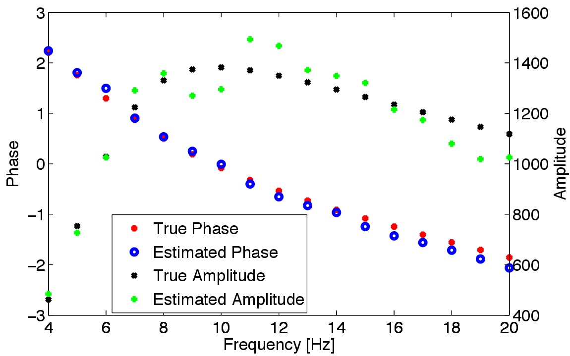
Figure 4 shows the comparison between the estimated source wavelet and the true source wavelet provided by Chevron. Aside from an obvious amplitude scaling, both the frequency-dependent phase and amplitude characteristics are extremely well recovered from this complex elastic data set. This is remarkable because our modeling engine is the scalar constant-density wave equation and this result is a clear illustration of the benefits of having a formulation where the physics and data are fitted jointly during the inversion. Considering both the difference between the inversion results and the true model and errors from the discretization, these slight differences between the true and estimated wavelet are acceptable.

Relation to existing work, discussion and summary

Discussion. Conceptually, the approach presented is related to the work of Baumstein (2013). There too, projections onto convex sets are used to regularize the waveform inversion problem. The optimization, computation of projections, as well as the sets are different. However, in that approach convergence may not be guaranteed because the projections are not guaranteed to be onto the intersections and because they only project at the end and do not solve constrained sub-problems. This is a problem when incorporating second-order information.

Tikhonov regularization is a well known regularization technique and adds quadratic penalties to objectives such as \(\min_\bm f(\bm) + \frac{\alpha}{2}\|R_1 \bm \|_2^2 + \frac{\beta}{2}\|R_2 \bm \|_2^2\), where two regularizers are used. The constants \(\alpha\) and \(\beta\) are the scalar weights, determining the importance of each regularizer. The matrices \(R\) represent properties of the model, which we would like to penalize. This method should in principle be able to achieve similar results as the projection approach, but it has a few disadvantages. The first one is that it may be difficult or costly to determine the weights \(\alpha\) and \(\beta\). Multiple techniques for finding a ‘good’ set of weights are available, including the L-curve, cross-validation and the discrepancy principle, see Sen and Roy (2003) for an overview in a geophysical setting. A second issue with the penalty approach is the effect of the penalty terms on the condition number of the Hessian of the optimization problem, see Nocedal and Wright (2000). This means that certain choices of \(\alpha\), \(\beta\), \(R_1\) and \(R_2\) may lead to an optimization problem which is infeasibly expensive to solve. A third issue is related to the two-norm squared, \(\| \cdot \|_2^2\) not being a so called ‘exact’ penalty function Nocedal and Wright (2000). This means that constraints can be approximated with the penalty functions, but generally not satisfied exactly. Note that the projection and quadratic penalty strategies for regularization can be easily combined as \(\min_{\bm} f(\bm)+ \frac{\alpha}{2}\|R_1 \bm \|_2^2 + \frac{\beta}{2}\|R_2 \bm \|_2^2 \quad \text{s.t.} \quad \bm \in \mathcal{C}_1 \bigcap \mathcal{C}_2\).

Multiple researchers, for example Brenders and Pratt (2007), use the concept of filtering the gradient. A gradient filter can be represented as applying a linear operation to the gradient step as \(\bm_{k+1}=\bm_k - \gamma F \nabla_{\bm}f(\bm)\). Brenders and Pratt (2007) apply a low-pass filter to the gradient to prevent high-wavenumber updates to the model while inverting low-frequency seismic data. A similar effect is achieved by the proposed framework and using the set defined in \(\ref{cnx_set_def2}\). The projection-based approach has the advantage that it generalizes to multiple constraints on the model in multiple domains, whereas gradient filtering does not. Restricting the model to be in a certain space is quite similar to reparametrization of the model.

Summary. To arrive at a flexible and versatile constrained algorithm for FWI, we combine Dyksta’s algorithm with a projected-Newton type algorithm capable of merging several regularization strategies including Tikhonov regularization, gradient filtering and reparameterization. While our approach could in certain cases yield equivalent results yielded by standard types of regularization, there are not guarantees for the latter. In addition, the parameter selections become easier because the parameters are directly related to the properties of the model itself rather than to balancing data fits and regularization. Application of Wavefield Reconstruction Inversion to Leeuwen and Herrmann (2013) to the blind-test Chevron 2014 dataset show excellent and we believe competitive results that benefit from imposing the smoothing constraint. While there is still a lot of room for improvement, these results are encouraging and were obtained without data preprocessing, excessive handholding and cosmetic “tricks”. The fact that we recover the wavelet accurately using an acoustic constant density only modeling kernel also shows the relative robustness of the presented method.