Regularizing waveform inversion by projection onto intersections of convex sets.

Introduction

Full-waveform inversion (FWI) involves solving a nonlinear optimization problem with the goal of matching observed data with predicted data by iteratively updating the estimate of the subsurface properties. This is an inverse problem and may require some form of regularization to yield solutions, which conform with our knowledge about the Earth at the survey location.

In this expanded abstract we propose a regularization strategy based on solving constrained problems by projection onto intersections of convex sets. We incorporate multiple pieces of prior information about the Earth into the FWI optimization scheme, in an approach similar to Baumstein (2013). This avoids the use of quadratic penalties. It is also shown how the constrained problem formulation incorporates several preexisting regularization ideas. Synthetic and field data examples show the effectiveness of the method.

Waveform inversion with regularization by projection onto the intersection of convex sets

In search of a flexible and easy to use framework, which can incorporate most existing ideas in the geophysical community to regularize the waveform inversion problem, we propose to base our framework on solving constrained optimization problems of the form \[ \begin{equation} \label{prob_constr} \min_{\bm} f(\bm) \quad \text{s.t.} \quad \bm \in \mathcal{C}_1 \bigcap \mathcal{C}_2. \end{equation} \] The model vector, \(\bm\) (often velocity), and the objective function can measure the difference between predicted data and observed data, \(f(\bm)=\frac{1}{2}\| P H(\bm)^{-1}\bq - \bd \|^2_2\) as is often used in FWI. \(H\) is the discretized Helmholtz equation, \(P\) restricts the wavefield to the receiver locations, \(\bq\) is the vector containing source function and location and \(\bd\) is the observed data. It is also possible to use other norms and objective functions, for example the unconstrained objective function corresponding to the Wavefield Reconstruction Inversion (WRI) approach (Leeuwen and Herrmann 2013): \(f(\bm)=\frac{1}{2}\| P \bar{\bu} - \bd \|^2_2 +\frac{\lambda^2}{2}\| H(\bm) \bar{\bu} - \bq \|^2_2\) with \(\bar{\bu}=(\lambda^2 H^*H + P^*P)^{-1} (\lambda^2 H^*\bq + P^* \bd)\).

\(\mathcal{C}_1\) and \(\mathcal{C}_2\) are convex sets (more than 2 sets can be used). Intuitively, the line connecting any two points in a convex set is also in the set: for all \(x\),\(y\) \(\in \mathcal{C}\) the following holds: \(c x +(1-c)y \in \mathcal{C}\), \(0 \leq c \leq 1\). Each set represents a known piece of information about the Earth; a constraint which the estimated model has to satisfy. The model is required to be in the intersection of the two sets, denoted by \(\mathcal{C}_1 \bigcap \mathcal{C}_2\). The intersection of convex sets is also convex. To summarize, solving Problem \(\ref{prob_constr}\) means we try to minimize the data misfit while satisfying constraints, which represent the known information about the geology. Below are two useful convex sets which are also used in the examples. Bound-constraints can be defined element-wise as \[ \begin{equation} \label{cnx_set_def1} \mathcal{C}_1 \equiv \{ \bm \: | \: \bb_l \leq \bm \leq \bb_u \}. \end{equation} \] If a model is in this set, then every model parameter value is between a lower bound \(\bb_l\) and upper bound, \(\bb_u\). These bounds can vary per model parameter and can therefore incorporate spatially-varying information about the bounds. Bound constraints can also incorporate a reference model by limiting the maximum deviation from this reference model as: \(\bb_l = \bm_{\text{ref}} - \delta\bm\). The projection onto \(\mathcal{C}_1\), denoted as \(\mathcal{P}_{\mathcal{C}_1}\), is the elementwise median: \(\mathcal{P}_{\mathcal{C}_1} (\bm)= \text{median}\{ \bb_l , \bm , \bb_u\}\).
The second convex set that is used here is a subset of the wavenumber domain representation of the model (spatial Fourier transformed). This convex set can be defined as \[ \begin{equation} \label{cnx_set_def2} \mathcal{C}_2 \equiv \{ \bm \: | \: E^*F^*(I-S)FE\bm=0\}. \end{equation} \] This set is defined by a series of matrix multiplications and means that we apply the mirror-extension operator, \(E\) to the model \(\bm\) to prevent wrap-around effects due to applying linear operations in the wavenumber domain. Next, the mirror extended model is spatially Fourier transformed using \(F\). In this domain we require the wavenumber content outside a certain range to be equal to zero. This is enforced by the diagonal (windowing) matrix \(S\). This represents information that the model should have a certain minimum smoothness. In case we expect an approximately horizontally layered medium without sharp contrasts, we can include this information by requiring the wavenumber content of the model to vanish outside of an elliptical zone around the zero wavenumber point (see also Brenders and Pratt (2007)). In other words, more smoothness in one direction is required than in the other direction. The adjoint of \(F\), (\(F^*\)) transforms back from the wavenumber to the physical domain and \(E^*\) goes from mirror-extended domain to the original model domain. The projection onto \(\mathcal{C}_2\), denoted as \(\mathcal{P}_{\mathcal{C}_2}\), is given by \(\mathcal{P}_{\mathcal{C}_2} (\bm)= E^*F^*SFE\bm\).

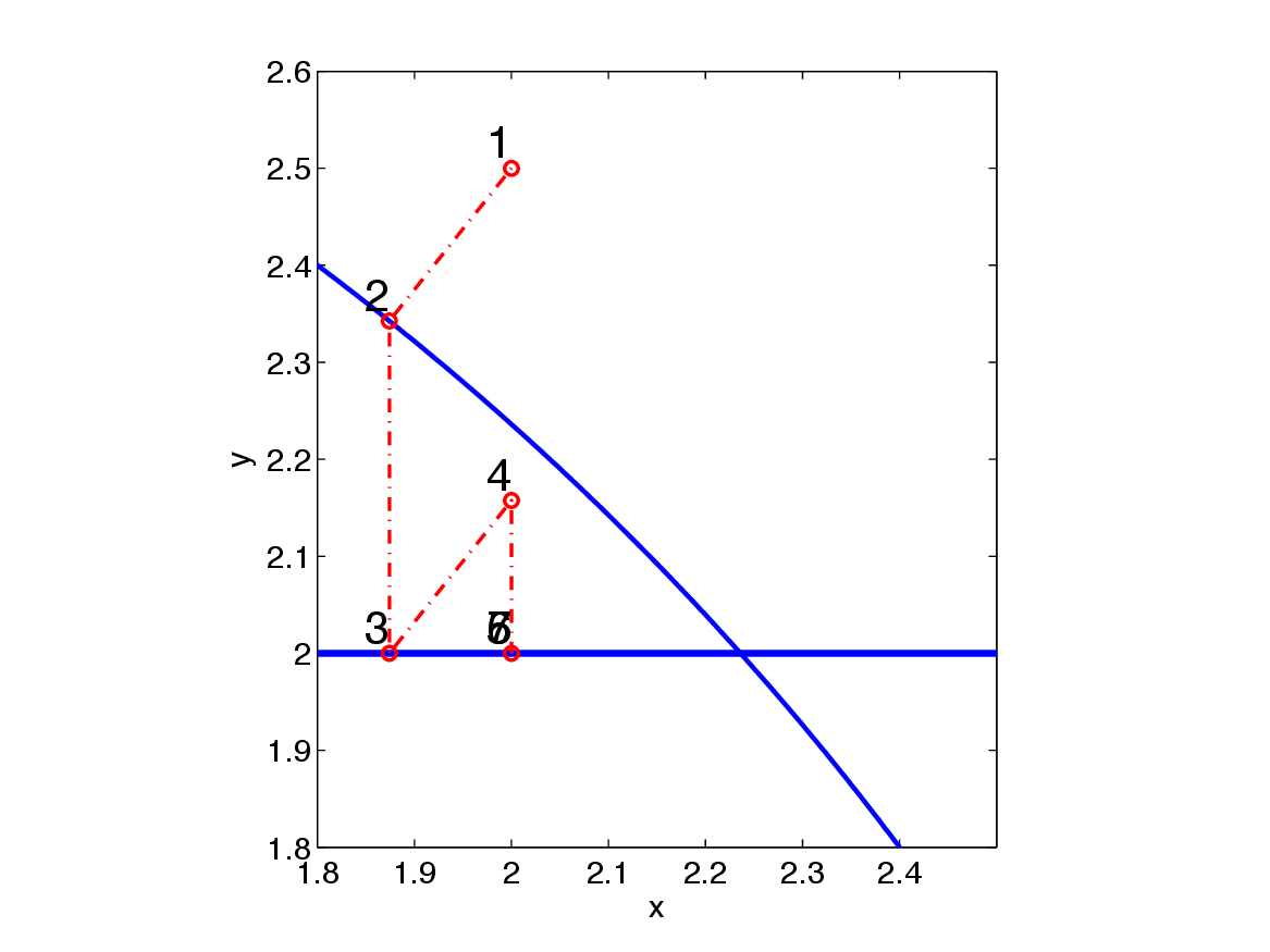
A basic way to solve Problem \(\ref{prob_constr}\) is to use the projected-gradient algorithm, which has the main step \(\bm_{k+1}=\mathcal{P}_{\mathcal{C}} (\bm_k - \gamma \nabla_{\bm}f(\bm))\), with a step length parameter \(\gamma\). \(\mathcal{P}_{\mathcal{C}}=\mathcal{P}_{\mathcal{C}_1 \bigcap \mathcal{C}_2}\) is the projection onto the intersection of all convex sets the model is required to be in. “The projection onto” means we need to find the point that is in both sets and closest to the current proposed model estimate generated by \((\bm_k - \gamma \nabla_{\bm}f(\bm))\). To find such a point, defined mathematically as \[ \begin{equation} \label{def_proj} \mathcal{P_{C}}({\bm})=\operatorname*{arg\,min}_{\mathbf{x}} \| \mathbf{x}-\bm \|_2 \quad \text{s.t.} \quad \mathbf{x} \in \mathcal{C}_1 \bigcap \mathcal{C}_2, \end{equation} \] we can use a splitting method such as Dykstra’s projection algorithm (Bauschke and Borwein 1994). This algorithm finds the projection onto the intersection of the two sets, by projecting onto each set separately. This is a cheap and simple algorithm and enables projections onto complicated intersections of sets. The algorithm is given by Algorithm 1.

While the gradient-projection algorithm is a solid approach, it can also be relatively slowly converging. A potentially much faster algorithm is the class of quasi-Newton methods, which iteratively try to approximate the Hessian by using just gradient and function value information. However, in general it is not possible to straightforwardly project quasi-Newton steps onto a convex set. The use of second-order information can cause the algorithm to converge to a solution which does not correspond to Problem \(\ref{prob_constr}\). There are slightly more complicated algorithms, which properly implement a second-order approach. We select the projected-quasi-Newton (PQN) algorithm by Schmidt et al. (2009). This algorithm finds a search direction which is in the intersection of the convex sets using the spectral projected gradient algorithm (SPG) as a sub-problem of an l-BFGS-like algorithm. It does not simply project an update. This algorithm needs the objective function value, \(f(\bm)\) , its gradient and an algorithm to solve the projection Problem \(\ref{def_proj}\). PQN has a very similar computational cost as the standard l-BFGS algorithm, because the projections are cheap to compute. See Schmidt et al. (2009) for some examples of strong empirical performance of PQN versus projected-gradient for some non-geophysical examples. The final algorithm is given by Algorithm 2.

Example 1: Inversion of very noisy data

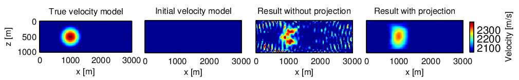
This is a synthetic example where the goal is to invert \(10\) Hz data with \(\| \text{noise} \|_2 / \|\text{signal}\|_2=0.3\). Inverting the noisy data will yield a noisy image, even if we use bound-constraints and a good start model. When the bound-constraints are used together with the projection onto set \(\mathcal{C}_{2}\), the inverted result is quite satisfying. The projection method is very effective for this type of situation, because the noise in the data induces highly oscillatory components in the model, which are outside the spatial Fourier spectrum of the expected model. Therefore, those components are projected out and can never enter the model. When used in this way, the projection onto \(\mathcal{C}_2\) can be interpreted as an image-domain noise filter. Besides the model-domain noise filter interpretation, the projection also keeps the model within the range of physically acceptable models. This restriction of the space, from \(\bm \in \mathbb{R}^N\) to \(\bm \in \mathcal{C}_1 \bigcap \mathcal{C}_2 \subset \mathbb{R}^N\) may prevent the optimization of \(f(\bm)\) to get stuck in local minimizers. Note that \(f(\bm)\) is unaltered by the projection approach, just the space where the model can be. The true model, initial model and results with and without projection onto \(\mathcal{C}_2\) are shown in Figure 2

Example 2: Land data in a vertical seismic profiling experiment

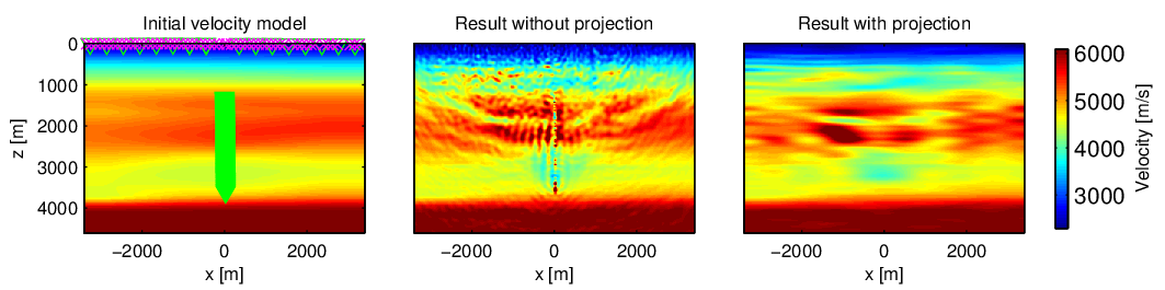
Vertical Seismic Profiling (VSP) data was acquired with receivers on the surface and in part of the well. The sources are on the surface only. Available data has a frequency content of \(8\) to \(15.75\) Hertz and all frequencies were used simultaneously in one batch. No density, elastic and attenuation effects are accounted for in the modeling. No significant anisotropy is expected in this type of geology from the Permian Basin.

The results are obtained by solving Problem \(\ref{prob_constr}\). The set \(\mathcal{C}_2\) is specified as follows. First the spatial Fourier spectrum of the initial model is analyzed. Then the filter \(S\) in Equation \(\ref{cnx_set_def2}\) is designed to allow the spatial Fourier spectrum of the initial model plus a bit higher spatial frequency content, based on what wavenumber spectrum can be expected from the startmodel in combination with the frequency content of the data. The results are shown in Figure 3.

Relation to existing work, discussion and summary

Conceptually, the approach presented is related to the work of Baumstein (2013). There too, projections onto convex sets are used to regularize the waveform inversion problem. The optimization, computation of projections, as well as the sets are different.

Tikhonov regularization is a well known regularization technique and adds quadratic penalties to an objective as \(\min_\bm f(\bm) + \frac{\alpha}{2}\|R_1 \bm \|_2^2 + \frac{\beta}{2}\|R_2 \bm \|_2^2\), where two regularizers are used. \(\alpha\) and \(\beta\) are the scalar weights, determining the importance of each regularizer. The matrices \(R\) represent properties of the model, which we would like to penalize. This method should in principle be able to achieve similar results as the projection approach, but it has a few disadvantages. The first one is that it may be difficult or costly to determine the weights \(\alpha\) and \(\beta\). Multiple techniques for finding a ‘good’ set of weights are available, including the L-curve, cross-validation and the discrepancy principle, see Sen and Roy (2003) for an overview in a geophysical setting. A second issue with the penalty approach is the effect of the penalty terms on the condition number of the Hessian of the optimization problem, see Nocedal and Wright (2000). This means that certain choices of \(\alpha\), \(\beta\), \(R_1\) and \(R_2\) may lead to an optimization problem which is infeasibly expensive to solve. A third issue is related to the two-norm squared, \(\| \cdot \|_2^2\) not being a so called ‘exact’ penalty function Nocedal and Wright (2000). This means that constraints can be approximated with the penalty functions, but generally not satisfied exactly. Note that the projection and quadratic penalty strategies for regularization can be easily combined as \(\min_{\bm} f(\bm)+ \frac{\alpha}{2}\|R_1 \bm \|_2^2 + \frac{\beta}{2}\|R_2 \bm \|_2^2 \quad \text{s.t.} \quad \bm \in \mathcal{C}_1 \bigcap \mathcal{C}_2\).

The concept of filtering the gradient is used by multiple researchers, for example Brenders and Pratt (2007). A gradient filter can be represented as applying a linear operation to the gradient step as \(\bm_{k+1}=\bm_k - \gamma F \nabla_{\bm}f(\bm)\). Brenders and Pratt (2007) apply a low-pass filter to the gradient to prevent high-wavenumber updates to the model while inverting low-frequency seismic data. A very similar effect is achieved by the framework proposed in this abstract and using the set defined in \(\ref{cnx_set_def2}\). The projection based approach has the advantage that it straightforwardly generalizes to multiple constraints on the model in multiple domains, whereas gradient filtering does not. Restricting the model to be in a certain space is quite similar to reparametrization of the model in, for example the (partial) spatial Fourier domain.

In summary, in this abstract we combine Dyksta’s algorithm with the projected quasi-Newton algorithm in order to merge several regularization strategies for waveform inversion, such as Tikhonov regularization, gradient filtering and reparameterization into one framework, which is simple to use and extend. Although the projection onto the intersection of multiple convex sets strategy does not necessarily yield better results than other regularization strategies, it may be easier to obtain improved results, because the projection approach makes is clear what constraints are satisfied exactly at every iteration. — csl: “/Tools/ScholarlyMarkdown-SLIM/csl/geophysics.csl” —