Total variation regularization strategies in full waveform inversion for improving robustness to noise, limited data and poor initializations

Disclaimer. This technical report is ongoing work (and posted as is except for the addition of another author) of the late John “Ernie” Esser (May 19, 1980 - March 8, 2015), who passed away under tragic circumstances. We will work hard to finalize and submit this work to the peer-review literature. Felix J. Herrmann

Introduction

Acoustic full waveform inversion (FWI) in the frequency domain can be written as the following PDE constrained optimization problem (Tarantola, 1984; Virieux and Operto, 2009; F. J. Herrmann et al., 2013) \[ \begin{equation} \min_{m,u} \sum_{sv} \frac{1}{2}\|P u_{sv} - d_{sv}\|^2 \ \ \text{s.t.} \ \ A_v(m)u_{sv} = q_{sv} \ , \label{PDEcon} \end{equation} \] where \(A_v(m)u_{sv} = q_{sv}\) denotes the discretized Helmholtz equation. Let \(s = 1,...,N_s\) index the sources and \(v = 1,...,N_v\) index frequencies. We consider the model, \(m\), which corresponds to the reciprocal of the velocity squared, to be a real vector \(m \in \R^{N}\), where \(N\) is the number of points in the spatial discretization. For each source and frequency the wavefields, sources and observed data are denoted by \(u_{sv} \in \C^N\), \(q_{sv} \in \C^N\) and \(d_{sv} \in \C^{N_r}\) respectively, where \(N_r\) is the number of receivers. \(P\) is the operator that projects the wavefields onto the receiver locations. The Helmholtz operator has the form \[ \begin{equation} A_v(m) = \omega_v^2 \diag(m) + L \ , \label{Helmholtz} \end{equation} \] where \(\omega_v\) is angular frequency and \(L\) is a discrete Laplacian.

The nonconvex constraint and large number of unknowns make (\(\ref{PDEcon}\)) a very challenging inverse problem. Since it is not always desirable to exactly enforce the PDE constraint, it was proposed in (T. van Leeuwen and Herrmann, 2013b, 2013a) to work with a quadratic penalty formulation of (\(\ref{PDEcon}\)), formally written as \[ \begin{equation} \min_{m,u} \sum_{sv} \frac{1}{2}\|P u_{sv} - d_{sv}\|^2 + \frac{\lambda^2}{2}\|A_v(m)u_{sv} - q_{sv}\|^2 \ . \label{penalty_formal} \end{equation} \] Their method will be referred to as Wavefield Reconstruction Inversion (WRI) and has been further studied in (Peters et al., 2014). The objective in (\(\ref{penalty_formal}\)) is formal in the sense that a slight modification is needed to properly incorporate boundary conditions, and this modification also depends on the particular discretization used for \(L\). As discussed in (T. van Leeuwen and Herrmann, 2013b; Peters et al., 2014), methods for solving the penalty formulation seem less prone to getting stuck in local minima when compared to solving formulations that require the PDE constraint to be satisfied exactly. The unconstrained problem is easier to solve numerically, with alternating minimization as well as Newton-like strategies being directly applicable. Moreover, since the wavefields are decoupled it isn’t necessary to store them all simultaneously when using alternating minimization approaches.

The most natural alternating minimization strategy is to iteratively solve the data augmented wave equation \[ \begin{equation} \bar{u}_{sv}(m^n) = \arg \min_{u_{sv}} \frac{1}{2}\|Pu_{sv} - d_{sv}\|^2 + \frac{\lambda^2}{2}\|A_v(m^n)u_{sv} - q_{sv}\|^2 \label{ubar} \end{equation} \] and then compute \(m^{n+1}\) according to \[ \begin{equation} m^{n+1} = \arg \min_m \sum_{sv} \frac{\lambda^2}{2}\|L\bar{u}_{sv}(m^n) + \omega_v^2 \diag(\bar{u}_{sv}(m^n))m - q_{sv}\|^2 \ . \label{m_altmin} \end{equation} \] This can be interpreted as a Gauss Newton method for solving \[ \begin{equation} \min_m F(m) , \label{Fmin} \end{equation} \] where \[ \begin{equation} F(m) = \sum_{sv}F_{sv}(m) \label{F} \end{equation} \] and \[ \begin{equation} F_{sv}(m) = \frac{1}{2}\|P \bar{u}_{sv}(m) - d_{sv}\|^2 + \frac{\lambda^2}{2}\|A_v(m)\bar{u}_{sv}(m) - q_{sv}\|^2 \ . \label{Fsv} \end{equation} \] Using a variable projection argument (Aravkin and Leeuwen, 2012), the gradient of \(F\) at \(m^n\) can be computed by \[ \begin{equation} \begin{aligned} \nabla F(m^n) & = \sum_{sv} \re\left( \lambda^2 \omega_v^2 \diag(\bar{u}_{sv}(m^n))^* \right.\\ & \left. (\omega_v^2 \diag(\bar{u}_{sv}(m^n))m^n + L\bar{u}_{sv}(m^n) - q_{sv})\right) \ . \end{aligned} \label{gradF} \end{equation} \] A scaled gradient descent approach (Bertsekas, 1999) for minimizing \(F\) can be written as \[ \begin{equation} \begin{aligned} \dm & = \arg \min_{\dm \in R^N} \dm^T \nabla F(m^n) + \frac{1}{2} \dm^T H^n \dm \\ m^{n+1} & = m^n + \dm \ , \end{aligned} \label{SGD} \end{equation} \] where \(H^n\) should be a positive definite approximation to the Hessian of \(F\) at \(m^n\). This general form includes gradient descent in the case when \(H^n=\frac{1}{\dt}\I\) for some time step \(\dt\) and Newton’s method when \(H^n\) is the true Hessian. In (T. van Leeuwen and Herrmann, 2013b), a Gauss Newton approximation is used with \[ \begin{equation} H^n = \sum_{sv} H_{sv}^n \ , \label{H} \end{equation} \] where \[ \begin{equation} H_{sv}^n = \re (\lambda^2 \omega_v^4 \diag(\bar{u}_{sv}(m^n))^*\diag(\bar{u}_{sv}(m^n)) \ . \label{Hsv} \end{equation} \] Since the Gauss Newton Hessian approximation is diagonal, it can be incorporated into (\(\ref{SGD}\)) with essentially no additional computational expense. This corresponds to the alternating procedure of iterating (\(\ref{ubar}\)) and (\(\ref{m_altmin}\)) at least for the formal objective that is linear in \(m\), which it may not be in practice depending on how the boundary conditions are implemented.

Including Convex Constraints

To make the inverse problem more well posed we can add the constraint \(m \in C\), where \(C\) is a convex set, and solve \[ \begin{equation} \min_m F(m) \ \text{ s.t. }\ m \in C \ . \label{Fmincon} \end{equation} \] For example, a box constraint on the elements of \(m\) could be imposed by setting \(C = \{m : m_i \in [b_i , B_i]\}\). The only modification of (\(\ref{SGD}\)) is to replace the \(\dm\) update by \[ \begin{equation} \begin{aligned} \dm & = \arg \min_{\dm \in R^N} \dm^T \nabla F(m^n) + \frac{1}{2} \dm^T H^n \dm \\ & \text{ s.t. }\ m^n + \dm \in C \ , \end{aligned} \label{dmcon} \end{equation} \] leading to a scaled gradient projection method (Bertsekas, 1999; Bonettini et al., 2009).

The constraint on \(\dm\) ensures \(m^{n+1} \in C\) but makes \(\dm\) more difficult to compute. Note that the simpler iterations \(m^{m+1} = \Pi_C(m^n - (H^n)^{-1}\nabla(F(m^n))\) obtained by first taking a scaled gradient descent step and then projecting onto \(C\) are not in general guaranteed to converge to a solution of (\(\ref{Fmincon}\)) (Bertsekas, 1999). The problem in (\(\ref{dmcon}\)) is still tractable if \(C\) is easy to project onto or can be written as an intersection of convex constraints that are each easy to project onto. As long as the projections can be computed efficiently, this convex subproblem is unlikely to be a computational bottleneck relative to the expense of solving for \(\bar{u}(m^n)\) (\(\ref{ubar}\)), and in fact it could even speed up the overall method if it leads to fewer required iterations.

The scaled gradient projection framework includes a variety of methods depending on the choice of \(H^n\). For example, if \(H^n=\frac{1}{\dt}\I\), (\(\ref{dmcon}\)) becomes a gradient projection iteration with a time step of \(\dt\). Projected Newton like methods are included when \(H^n\) is chosen to approximate the Hessian of \(F\) at \(m^n\). A good summary of some of the possible methods in this framework can be found in (Mark Schmidt et al., 2012). In particular, a robust projected quasi Newton method proposed in (MW Schmidt, 2009) uses a limited memory BFGS approximation of the Hessian and solves the convex subproblems for each update with a spectral projected gradient method.

For the particular application of minimizing the WRI objective subject to additional convex constraints (\(\ref{Fmincon}\)), we will prefer to use projected Gauss Newton or Levenberg Marquardt type iterations because the Gauss Newton Hessian approximation for the WRI objective is diagonal. Projected gradient based methods for solving the convex subproblems are reasonable when the constraint sets are easy to project onto. However, since one of the constraints we would like to impose is a bound on the total variation (TV) of the model \(m\), the resulting convex subproblems for computing the updates can be more naturally solved by methods that incorporate operator splitting to simplify the projection. Another consideration when solving (\(\ref{Fmincon}\)) is that line search can potentially be expensive because evaluating \(F(m)\) requires first solving a large linear system for \(\bar{u}(m)\). Instead of doing a line search for each search direction, we prefer to introduce a damping parameter by replacing \(H^n\) with \(H^n + c_n\I\) and adaptively adjust \(c_n\) at each iteration, rejecting iterations that don’t lead to a sufficient decrease in the objective.

If \(\nabla F\) is Lipschitz continuous, so that for some \(K\) \[ \begin{equation*} \|\nabla F(x) - \nabla F(y)\| \leq K \|x - y\| \ \text{for all } x,y \in C , \end{equation*} \] and if \(H\) is a symmetric matrix, then \(c\) can be chosen large enough so that \[ \begin{equation} F(m+\dm) - F(m) \leq \dm^T \nabla F(m) + \frac{1}{2} \dm^T (H + c\I)\dm \label{majmin} \end{equation} \] for any \(m \in C\) and \(\dm\) such that \(m + \dm \in C\). So for large enough \(c_n\), \(F(m^n+\dm) \leq F(m^n)\) when \(\dm\) is defined by (\(\ref{dmcon}\)). In particular since \[ \begin{equation*} F(m+\dm) - F(m) \leq \dm^T \nabla F(m) + \frac{K}{2}\|\dm\|^2 \ , \end{equation*} \] it follows that \[ \begin{equation*} \begin{aligned} F(m+\dm) - F(m) & \leq \frac{1}{2}(K - \lambda_H^{\text{min}} - c)\|\dm\|^2 + \\ & \dm^T \nabla F(m) + \frac{1}{2} \dm^T (H + c\I)\dm \ , \end{aligned} \end{equation*} \] where \(\lambda_H^{\text{min}}\) denotes the smallest eigenvalue of \(H\). So choosing \(c > K - \lambda_H^{\text{min}}\) would ensure that (\(\ref{majmin}\)) is satisfied. This would, however, be an extremely conservative choice of the damping parameter \(c\), which could lead to a slow rate of convergence. We can also adaptively choose \(c_n\) to be as small as possible while still leading to iterations that decrease the objective by a sufficient amount, namely such that \[ \begin{equation} F(m+\dm) - F(m) \leq \sigma (\dm^T \nabla F(m) + \frac{1}{2} \dm^T (H + c\I)\dm) \ , \label{suffdec} \end{equation} \] for some \(\sigma \in (0,1]\). Using the same framework as in (E. Esser et al., 2013), the resulting method is summarized in Algorithm 1.

The particular choice of \(H^{n}\) we will use is the Gauss Newton Hessian defined by Equations \(\ref{H}\) and \(\ref{Hsv}\). Other choices are also possible, but if \(H^n\) is a poor approximation to the Hessian of \(F\) at \(m^n\), then a larger damping parameter \(c_n\) may be needed. Note that \(c_n\) will remain bounded because any \(c_n > K - \lambda_H^{\text{min}}\) would guarantee a sufficient decrease of \(F\).

In addition to assuming \(\nabla F\) is Lipschitz continuous, suppose \(F(m)\) is coercive on \(C\) so that for any \(m \in C\), \(\{\tilde{m} \in C : F(\tilde{m}) \leq F(m) \}\) is bounded. Then it follows that any limit point \(m^*\) of the sequence of iterates \(\{m^n\}\) defined by Algorithm 1 is a stationary point of (\(\ref{Fmincon}\)) in the sense that \((m - m^*)^T \nabla F(m^*) \geq 0\) for all \(m \in C\).

When \(H^n + c_n\I\) is diagonal and positive, which it is for the Gauss Newton Hessian defined by (\(\ref{H}\)), it’s straightforward to add the spatially varying bound constraint \(m_i \in [b_i , B_i]\). In fact \[ \begin{equation} \begin{aligned} \dm & = \arg \min_{\dm} \dm^T \nabla F(m^n) + \frac{1}{2}\dm^T (H^n + c_n \I) \dm \\ & \text{s.t.} \ m^n_i + \dm_i \in [b_i, B_i] \end{aligned} \label{bounds} \end{equation} \] has the closed form solution \[ \begin{equation*} \dm_i = \max\left(b_i - m^n_i,\min\left(B_i - m^n_i,-[(H^n + c_n \I)^{-1}\nabla F(m^n)]_i \right) \right) \ . \end{equation*} \] Even with bound constraints, the model recovered using the penalty formulation can still contain artifacts and spurious oscillations, as shown for example in Figure 4. A simple and effective way to reduce oscillations in \(m\) via a convex constraint is to constrain its total variation to be less than some positive parameter \(\tau\). TV penalties are widely used in image processing to remove noise while preserving discontinuities (Rudin et al., 1992). It is also a useful regularizer in a variety of other inverse problems, especially when solving for piecewise constant or piecewise smooth unknowns. For example, TV regularization has been successfully used for electrical inverse tomography (Chung et al., 2005) and inverse wave propagation (Akcelik et al., 2002). Although the problem is similar, the formulation in (Akcelik et al., 2002) is different in that they directly penalize the total variation of the velocity instead of constraining the total variation of the slowness squared. Total variation regularization has also been successfully used in other recent extensions of full waveform inversion. It is used to regularize the inversion of time lapse seismic data in (Maharramov and Biondi, 2014). It is also embedded in model updates to encourage blocky models in an FWI method that includes shape optimization in (Guo and Hoop, 2012).

Total Variation Regularization

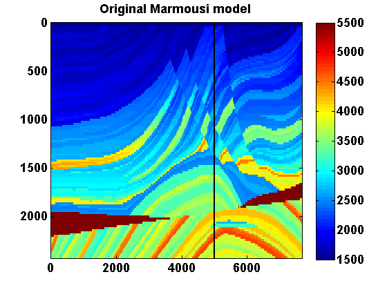
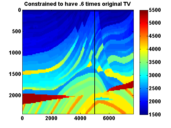
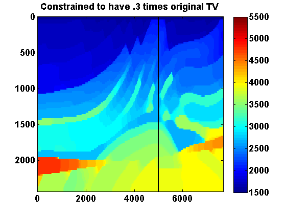
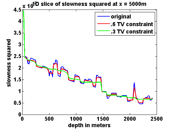
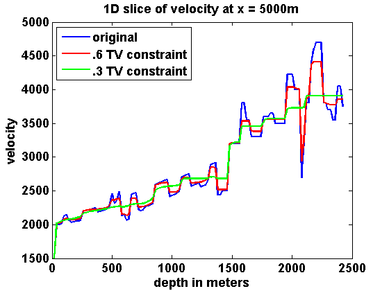
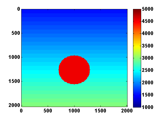
If we represent \(m\) as a \(N_1\) by \(N_2\) image, we can define \[ \begin{equation} \begin{aligned} \|m\|_{TV} & = \frac{1}{h}\sum_{ij}\sqrt{(m_{i+1,j}-m_{i,j})^2 + (m_{i,j+1}-m_{i,j})^2} \\ & = \sum_{ij}\frac{1}{h}\left\| \bbm (m_{i,j+1}-m_{i,j})\\ (m_{i+1,j}-m_{i,j}) \ebm \right\| \ , \end{aligned} \label{TVim} \end{equation} \] which is a sum of the \(l_2\) norms of the discrete gradient at each point in the discretized model. Assume Neumann boundary conditions so that these differences are zero at the boundary. We can represent \(\|m\|_{TV}\) more compactly by defining a difference operator \(D\) such that \(Dm\) is a concatenation of the discrete gradients and \((Dm)_n\) denotes the vector corresponding to the discrete gradient at the location indexed by \(n\), \(n = 1,...,N_1N_2\). Then we can define \[ \begin{equation} \|m\|_{TV} = \|Dm\|_{1,2} := \sum_{n=1}^N \|(Dm)_n\| \ . \label{TVvec} \end{equation} \] Returning to (\(\ref{SGD}\)), if we add the constraints \(m_i \in [b_i , B_i]\) and \(\|m\|_{TV} \leq \tau\), then the overall iterations for solving \[ \begin{equation} \min_m F(m) \qquad \text{s.t.} \qquad m_i \in [b_i , B_i] \text{ and } \|m\|_{TV} \leq \tau \label{QP} \end{equation} \] have the form \[ \begin{equation} \begin{aligned} \dm & = \arg \min_{\dm} \dm^T \nabla F(m^n) + \frac{1}{2}\dm^T (H^n + c_n\I) \dm \\ & \text{s.t. } m^n_i + \dm_i \in [b_i , B_i] \text{ and } \|m^n + \dm\|_{TV} \leq \tau \\ m^{n+1} & = m^n + \dm \ . \end{aligned} \label{pTVb} \end{equation} \] To illustrate the effect of the TV constraint, consider projecting the Marmousi model shown in Figure 1a onto two sets with total variation constraints using different values of \(\tau\). Let \(m_0\) denote the Marmousi model and let \(\tau_0 = \|m_0\|_{TV}\). For the bound constraints, set \(B_i = 4.4444\e{-7}\) everywhere, which corresponds to a lower bound of \(1500\) on the velocity. Taking advantage of the fact that these constraints can vary spatially, let \(b_i = 4.4444\e{-7}\) in the water layer and \(b_i = 3.3058\e{-8}\) everywhere else, which corresponds to an upper bound of \(5500\) on the velocity. The orthogonal projection of \(m_0\) onto the intersection of these box and TV constraints is defined by \[ \begin{equation} \begin{aligned} \Pi_C(m_0) & = \arg \min_m \frac{1}{2} \|m - m_0\|^2 \\ & \text{s.t. } m_i \in [b_i , B_i] \text{ and } \|m\|_{TV} \leq \tau \ . \end{aligned} \label{proj_C} \end{equation} \] Results with \(\tau = .6\tau_0\) and \(\tau = .3\tau_0\) are shown in Figure 1. The vertical lines at \(x = 5000\)m indicate the location of the 1D depth slices shown in Figure 2 for both slowness squared and velocity.

A weighted version of the TV constraint can be obtained by replacing \(D\) with \(\Gamma D\) for some positive diagonal matrix \(\Gamma\). This could for instance be used to make the strength of the TV constraint vary with depth.

Solving the Convex Subproblems

An effective approach for solving the convex subproblems in (\(\ref{pTVb}\)) for \(\dm\) is to use a modification of the primal dual hybrid gradient (PDHG) method (Zhu and Chan, 2008) studied in (E. Esser et al., 2010; Chambolle and Pock, 2011; He and Yuan, 2012; Zhang et al., 2010) to find a saddle point of \[ \begin{equation} \begin{aligned} \L(\dm,p) & = \dm^T \nabla F(m^n) + \frac{1}{2}\dm^T (H^n + c_n\I) \dm + g_B(m^n + \dm)\\ & + p^T D(m^n + \dm) - \tau \|p\|_{\infty,2} \end{aligned} \label{Lagrangian} \end{equation} \] where \(g_B\) is an indicator function for the bound constraints, \[ \begin{equation*} g_B(m) = \begin{cases} 0 & \text{ if } m_i \in [b_i , B_i] \\ \infty & \text{ otherwise} \end{cases}. \end{equation*} \] Here, \(\|\cdot\|_{\infty,2}\) is using mixed norm notation to denote the dual norm of \(\|\cdot\|_{1,2}\). It takes the max instead of the sum of the \(l_2\) norms so that \(\|Dm\|_{\infty,2} = \max_n \|(Dm)_n\|\) in the notation of Equation \(\ref{TVvec}\). The saddle point problem can be derived from the convex subproblem in (\(\ref{pTVb}\)) by representing the TV constraint as \[ \begin{equation} \sup_p p^T D(m^n + \dm) - \tau \|p\|_{\infty,2} \ , \label{TVsp} \end{equation} \] which equals the indicator function \[ \begin{equation*} \begin{cases} 0 & \text{ if } \|D(m^n + \dm)\|_{1,2} \leq \tau \\ \infty & \text{ otherwise} \end{cases}. \end{equation*} \] To find a saddle point of (\(\ref{Lagrangian}\)), the modified PDHG method requires iterating \[ \begin{equation} \begin{aligned} p^{k+1} & = \arg \min_p \tau \|p\|_{\infty,2} - p^T D(m^n + \dm^k) + \frac{1}{2 \delta}\|p - p^k\|^2 \\ \dm^{k+1} & = \arg \min_{\dm} \dm^T \nabla F(m^n) + \frac{1}{2}\dm^T (H^n + c_n\I) \dm \\ & + \dm^T D^T(2p^{k+1}-p^k) + \frac{1}{2 \alpha}\|\dm - \dm^k\|^2 \\ & \text{s.t. } m^n_i + \dm_i \in [b_i , B_i] \ . \end{aligned} \label{PDHGM} \end{equation} \] These iterations can be written more explicitly as \[ \begin{equation} \begin{aligned} p^{k+1} & = p^k + \delta D(m^n + \dm^k) - \Pi_{\|\cdot\|_{1,2} \leq \tau \delta}(p^k + \delta D(m^n + \dm^k)) \\ \dm^{k+1}_i & = \max\left( (b_i - m^n_i), \min\left( (B_i - m^n_i), \right. \right. \\ & \left. \left. [(H^n + (c_n+\frac{1}{\alpha})\I)^{-1}(-\nabla F(m^n) + \frac{\dm^k}{\alpha} - D^T(2p^{k+1}-p^k))]_i \right) \right) \ , \end{aligned} \label{PDHGexplicit} \end{equation} \] where \(\Pi_{\|\cdot\|_{1,2} \leq \tau \delta}(z)\) denotes the orthogonal projection of \(z\) onto the ball of radius \(\tau \delta\) in the \(\|\cdot\|_{1,2}\) norm. Computing this projection involves projecting the vector of \(l_2\) norms onto a simplex, which can be done in linear time (Brucker, 1984). An easy way to compute the orthogonal projection of a vector \(z\) onto the unit simplex \(\{x : x_i \geq 0 , \sum_i x_i = 1\}\) is to simply use bisection to find the threshold \(a\) such that \(\sum_i \max(0,z_i - a) = 1\), in which case \(\max(0,z_i - a)\) is the ith component of the projection.

The step size restriction required for convergence is \(\alpha \delta \leq \frac{1}{\|D^TD\|}\). If \(h\) is the mesh width, then the eigenvalues of \(D^TD\) are between \(0\) and \(\frac{8}{h^2}\) by the Gershgorin Circle Theorem, so it suffices to choose positive \(\alpha\) and \(\delta\) such that \(\alpha \delta \leq \frac{h^2}{8}\). In the weighted TV case, the same bound works as long as the weights are normalized so that they are all less than or equal to one in magnitude. Then the step size restriction \(\alpha \delta < \frac{h^2}{8}\) that was used for the unweighted TV constraint will also satisfy \(\alpha \delta < \frac{1}{\|\Gamma D\|^2}\), which is the step size restriction when the TV constraint is weighted by the diagonal matrix \(\Gamma\).

The relative scaling of \(\alpha\) and \(\delta\) can have a large effect on the convergence rate of the method. A reasonable choice of fixed step size parameters is \(\alpha = \frac{1}{\max(H^n + c_n\I)}\) and \(\delta = \frac{h^2 \max(H^n +c_n\I)}{8} \leq \frac{\max(H^n + c_n\I)}{\|D^TD\|}\). However, this choice may be too conservative. The convergence rate of the method can be improved by using the iteration dependent step sizes proposed in (Chambolle and Pock, 2011). The adaptive backtracking strategy proposed in (Goldstein et al., 2013) can also be a practical way of choosing efficient step size parameters.

Curvelet Sparsity

The total variation constraint penalizes the \(l_1\) norm of the gradient of \(m\) in order to promote sparsity of the gradient. Sparsity in other domains can also be encouraged using the same framework. For example, if \(\mathcal{C}\) denotes a curvelet transform, we can replace the discrete gradient \(D\) in the TV constraint with \(\mathcal{C}\) and encourage the curvelet coefficients of \(m\) to be sparse via the constraint \(\|\mathcal{C}m\|_1 \leq \tau\), which limits the sum of the absolute values of complex curvelet coefficients.

One-Sided TV Constraint

Since velocity generally increases with depth, it is natural to penalize downward jumps in velocity. This can be done with a one-sided, one dimensional total variation constraint that penalizes increases in the slowness squared in the depth direction. Such a constraint naturally fits in the same framework previously used to impose TV constraints. Define a forward difference operator \(D_z\) that acts in the depth direction so that \(D_z m\) is a concatenation of differences of the form \(\frac{1}{h}(m_{i+1,j} - m_{i,j})\). To penalize the sum of the positive differences in \(m\), we can include the constraint \[ \begin{equation} \|\max(0,D_z m)\|_1 \leq \xi \ , \label{HL} \end{equation} \] where \(\max\) is understood in a componentwise sense so that \(\|\max(0,D_z m)\|_1 = \sum_{ij} \max(0,\frac{1}{h}(m_{i+1,j} - m_{i,j}))\). This constraint is closely related to the hinge loss penalty commonly used for example in machine learning models such as support vector machines.

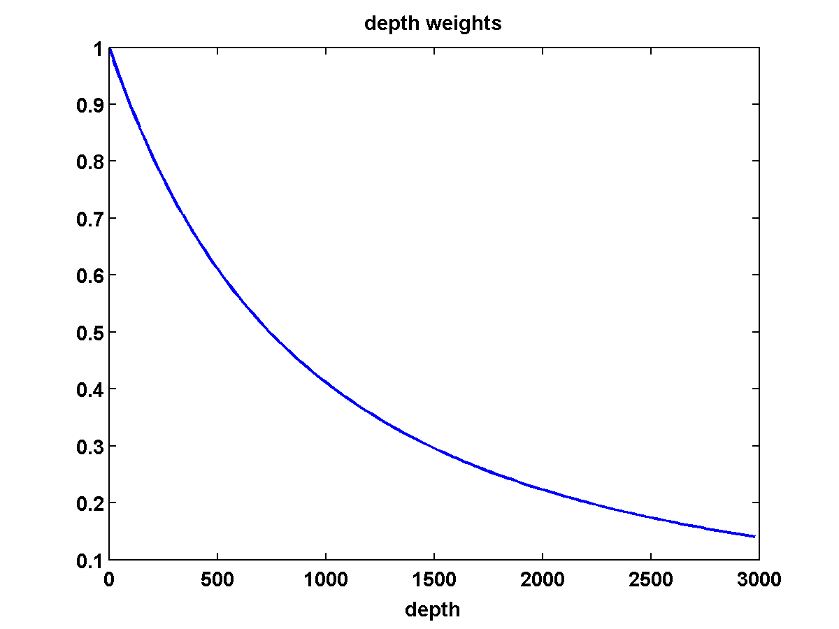
It’s also possible to include positive depth weights \(\gamma_i\) in the one-sided TV constraint, so that it becomes \[ \begin{equation} \sum_{ij} \max(0,\frac{\gamma_i}{h}((m_{i+1,j} - m_{i,j})) \leq \xi \ , \label{HLdpw} \end{equation} \] which also corresponds to replacing \(D_z\) by \(\Gamma D_z\) for a positive, diagonal matrix \(\Gamma\) with \(\gamma_i\) repeated along the diagonal. Using weights that decrease with depth may for example encourage deeper placement of discontinuities that still fit the data.

The constraint in (\(\ref{HL}\)) doesn’t penalize model discontinuities in the horizontal direction, only in the depth direction. It’s therefore likely to lead to vertical artifacts unless combined with additional regularization. It can for example be combined with a TV constraint.

The combination of TV and one-sided TV constraints still fits in same basic framework. Problem (\(\ref{QP}\)) becomes \[ \begin{equation} \min_m F(m) \ \ \text{s.t.} \ \ m_i \in [b_i , B_i] \text{ , } \|m\|_{TV} \leq \tau \text{ and } \|\max(0,D_z m)\|_1 \leq \xi \label{QP3} \end{equation} \] and the convex subproblems (\(\ref{pTVb}\)) that need to be solved are the same except for the added one-sided TV constraint, \[ \begin{equation} \begin{aligned} \dm & = \arg \min_{\dm} \dm^T \nabla F(m^n) + \frac{1}{2}\dm^T (H^n + c_n\I) \dm \\ & \text{s.t. } m^n_i + \dm_i \in [b_i , B_i] \text{ , } \|m^n + \dm\|_{TV} \leq \tau \\ & \text{ and } \|\max(0,D_z (m^n + \dm))\|_1 \leq \xi \ . \end{aligned} \label{pTVb3} \end{equation} \] The same method for solving the convex subproblems can be used. Analogous to (\(\ref{Lagrangian}\)), we want to find a saddle point of the Lagrangian \[ \begin{equation} \begin{aligned} \L(\dm,p_1,p_2) & = \dm^T \nabla F(m^n) + \frac{1}{2}\dm^T (H^n + c_n\I) \dm + g_B(m^n + \dm) \\ & + p_1^T D(m^n + \dm) - \tau \|p_1\|_{\infty,2} \\ & + p_2^T D_z(m^n + \dm) - \xi \max(p_2) - g_{\geq 0}(p_2) \ , \end{aligned} \label{Lagrangian3} \end{equation} \] where \(g_{\geq 0}\) denotes an indicator function defined by \[ \begin{equation*} g_{\geq 0}(p_2) = \begin{cases} 0 & \text{if } p_2 \geq 0 \\ \infty & \text{ otherwise } \end{cases}. \end{equation*} \] The extra terms in this Lagrangian compared to (\(\ref{Lagrangian}\)) follow from replacing the one-sided TV constraint by \[ \begin{equation} \sup_{p_2} p_2^T D_z (m^n + \dm) - \xi \max(p_2) - g_{\geq 0}(p_2) \ , \label{TV1sp} \end{equation} \] which equals the indicator function \[ \begin{equation*} \begin{cases} 0 & \text{ if } \|\max(0,D_z(m^n + \dm)\|_1 \leq \xi \\ \infty & \text{ otherwise} \end{cases}. \end{equation*} \] This can also be seen by noting that \(\xi \max(p) + g_{\geq 0}(p)\) is the Legendre transform of the indicator function \[ \begin{equation*} \begin{cases} 0 & \text{ if } \|\max(0,p)\|_1 \leq \xi \\ \infty & \text{ otherwise} \end{cases}. \end{equation*} \] The modified PDHG iterations are also similar. The update for \(p_1\) is the same as in (\(\ref{PDHGexplicit}\)). The update for \(p_2\) is very similar, and there is an extra term involving \(p_2\) in the \(\dm\) update. Altogether, the iterations are given by \[ \begin{equation} \begin{aligned} p_1^{k+1} & = p_1^k + \delta D(m^n + \dm^k) - \Pi_{\|\cdot\|_{1,2} \leq \tau \delta}(p_1^k + \delta D(m^n + \dm^k)) \\ p_2^{k+1} & = p_2^k + \delta D_z(m^n + \dm^k) - \Pi_{\|\max(0,\cdot)\|_1 \leq \xi \delta}(p_2^k + \delta D_z(m^n + \dm^k)) \\ \dm^{k+1}_i & = \max\left( (b_i - m^n_i), \min\left( (B_i - m^n_i), \right. \right. \\ & \left. \left. [(H^n + (c_n+\frac{1}{\alpha})\I)^{-1}(-\nabla F(m^n) + \frac{\dm^k}{\alpha} - \right. \right. \\ & \left. \left. D^T(2p_1^{k+1}-p_1^k) - D_z^T(2p_2^{k+1}-p_2^k))]_i \right) \right) \ . \end{aligned} \label{PDHGexplicit3} \end{equation} \] The projection \(\Pi_{\|\max(0,\cdot)\|_1 \leq \xi \delta}(z)\) can be computed by projecting the positive part of \(z\), \(\max(0,z)\), onto the simplex defined by \(\{z : z_j \geq 0 \ , \ \sum_j z_j = \xi \delta\}\) if it doesn’t already satisfy the constraint.

Adjoint State Formulation

All the above constraints can also be incorporated into an adjoint state formulation the PDE constrained problem in (\(\ref{PDEcon}\)) in which the Helmholtz equation must be exactly satisfied. The overall problem including a general convex constraint \(m \in C\) is given by \[ \begin{equation} \min_{m,u} \sum_{sv} \frac{1}{2}\|P u_{sv} - d_{sv}\|^2 \ \ \text{s.t.} \ \ A_v(m)u_{sv} = q_{sv} \ \ \text{and}\ \ m \in C \ . \label{PDEcon2} \end{equation} \] In place of \(F(m)\) defined by (\(\ref{Fsv}\)), define \[ \begin{equation} \tilde{F}_{sv}(m) = \frac{1}{2}\|P \tilde{u}_{sv}(m) - d_{sv}\|^2 \ , \label{ASFsv} \end{equation} \] where \(\tilde{u}(m)\) solves the Helmholtz equation \(A_v(m)\tilde{u}_{sv} = q_{sv}\). The objective can again be written as a sum over frequency and source indices, \[ \begin{equation} \tilde{F}(m) = \sum_{sv}\tilde{F}_{sv}(m) \ . \label{ASF} \end{equation} \] Using the adjoint state method, the gradient of \(\tilde{F}(m)\) can be written as \[ \begin{equation} \nabla \tilde{F}(m) = \sum_{sv} \re\left[ (\partial_m A_v(m))\tilde{u}_{sv}(m) \right]^* \tilde{v}_{sv}(m) \ , \label{gradASF} \end{equation} \] where \[ \begin{equation*} A_v(m)^*\tilde{v}_{sv}(m) = P^T(d_{sv} - P\tilde{u}_{sv}(m)) \ . \end{equation*} \] Formally, with \(A_v(m)\) defined by (\(\ref{Helmholtz}\)), \[ \begin{equation} \nabla \tilde{F}(m) = \sum_{sv} \re (\omega_v^2 \diag(\tilde{u}_{sv}(m))^* \tilde{v}_{sv}(m)) \ , \label{gradASF_formal} \end{equation} \] but this may require modification depending on how the boundary conditions are implemented. When designing a scaled gradient projection method analogous to (\(\ref{dmcon}\)) for minimizing \(\tilde{F}(m)\) subject to \(m \in C\) we can choose \[ \begin{equation} H^n = \sum_{sv} \re (\omega_v^4 \diag(\tilde{u}_{sv}(m^n))^*\diag(\tilde{u}_{sv}(m^n)) \label{HAS} \end{equation} \] even though it no longer corresponds to the Gauss Newton Hessian. Since we expect the structure of this positive diagonal Hessian approximation to be good but possibly scaled incorrectly, we may want to modify how the adaptive damping parameter \(c_n\) is implemented so that it automatically finds a good rescaling of \(H^n\). One possibility is to replace every instance of \(H^n + c_n\I\) in Algorithm 1 with \(c_n(H^n + \nu\I)\) for some small positive \(\nu\). With this substitution, the convex subproblems are exactly the same as in the WRI quadratic penalty formulation.

Numerical Experiments

We consider four 2D numerical FWI experiments based on synthetic data. All examples use a frequency continuation strategy that works with small subsets of frequency data at a time, moving gradually from low to high frequency batches.

In the first example, noisy data is generated based on a simple synthetic velocity model with sources and receivers placed vertically on the left and right sides of the model respectively, analogous to the transmission cross-well example in (Leeuwen and Herrmann, 2013). Here the TV constraint is effective in removing artifacts caused by the added noise.

In the second example, very few simultaneous shots are used to simulate data based on the SEG/EAGE salt model. With a good initial model, the TV constraint is helpful in removing artifacts caused by the use of so few simultaneous shots.

The third example is based on top left portion of the 2004 BP velocity benchmark data set (Billette and Brandsberg-Dahl, 2005). Due to the large salt body, the inversion results tend to have artifacts even when the initial model is good. In particular, the deeper part of the estimated model tends to have incorrect discontinuities. The TV constraint helps smooth out some of these artifacts while still recovering the most significant discontinuities. It can also help to compute multiple passes through the frequency batches while relaxing the TV constraint. A stronger TV constraint may initially result in an oversmoothed model estimate, but such an estimate can still be a good initial model when computing another pass with a weaker TV constraint.

The fourth example is based on the top middle portion of the same BP velocity model and shows how the one-sided TV constraint can be used to make the inversion results robust to a poor initial model. A continuation strategy that at first strongly discourages downward jumps in the estimated velocity helps prevent the method from getting stuck in bad local minima. By gradually relaxing the constraint, downward jumps in velocity are more tolerated during later passes through the frequency batches.

Before presenting the numerical examples, we first provide additional details about the discretization, boundary conditions and frequency continuation strategy.

Discretization and Boundary Conditions

The discrete Laplacian \(L\) in the Helmholtz operator (\(\ref{Helmholtz}\)) is defined using a simple five point stencil. We use a Robin boundary condition that can be written in the frequency domain as \[ \begin{equation} \nabla u_{sv} \cdot n = -i \omega_v \sqrt{m} u_{sv} \ . \label{RobinBC} \end{equation} \] To implement this, \(L\) is defined with Neumann boundary conditions, which effectively removes the differences at the boundary. Using the Robin boundary condition, these differences are then replaced by \(-i \omega \sqrt{m} u\). The boundary condition is incorporated into the objective (\(\ref{penalty_formal}\)) by replacing the PDE misfit penalties \[ \begin{equation*} \frac{\lambda^2}{2}\|Lu_{sv} + \omega_v^2 \diag(m)u_{sv} - q_{sv}\|^2 \end{equation*} \] with \[ \begin{equation*} \frac{\lambda^2}{2}\|Lu_{sv} + \omega_v^2 X_{\text{int}} \diag(m)u_{sv} -i \omega_v X_{\text{bnd}} \diag(\sqrt{m})u_{sv} - q_{sv}\|^2 \ , \end{equation*} \] where \(X_{\text{int}}\) is a mask represented as a diagonal matrix with ones corresponding to points in the interior and zeros corresponding to points on the boundary. Similarly, \(X_{\text{bnd}}\) is a diagonal matrix with values of zero for interior points, \(\frac{1}{h}\) for boundary edges and \(\frac{2}{h}\) at the corners. This boundary condition is used when computing \(\bar{u}_{sv}(m^n)\) (\(\ref{ubar}\)). The formulas for the gradient (\(\ref{gradF}\)) and the diagonal Gauss Newton Hessian (\(\ref{H}\)) corresponding to (\(\ref{Fsv}\)) are also modified accordingly. The gradient becomes \[ \begin{equation} \begin{aligned} \nabla F(m^n) & = \sum_{sv} \re\left( \lambda^2 \omega_v \diag(\bar{u}_{sv}(m^n))^*(\omega_v^3 X_{\text{int}} \diag(\bar{u}_{sv}(m^n)) + \right. \\ & \left. \omega_v X_{\text{int}}(L\bar{u}_{sv}(m^n)-q_{sv}) + \frac{i}{2}X_{\text{bnd}} \diag(m^{\frac{-1}{2}})(L\bar{u}_{sv}(m^n) - q_{sv}) + \right. \\ & \left. \frac{\omega_v}{2}X_{\text{bnd}}^2 \bar{u}_{sv}(m^n)) \right) \ , \end{aligned} \label{BCgradF} \end{equation} \] and the Gauss Newton Hessian becomes \[ \begin{equation} \begin{aligned} H^n & = \sum_{sv} \re\left( \lambda^2 \omega_v^4 X_{\text{int}} \diag(\bar{u}_{sv}(m^n))^*\diag(\bar{u}_{sv}(m^n)) - \right. \\ & \left. \frac{i w \lambda^2}{4} X_{\text{bnd}} \diag(m^{\frac{-3}{2}}) \diag(\conj(\bar{u}_{sv}(m^n))) \diag(L\bar{u}_{sv}(m^n) - q_{sv}) \right) \ . \end{aligned} \label{BCH} \end{equation} \]

Frequency Continuation

We choose to work with small batches of frequency data at a time, moving from low to high frequencies in overlapping batches of two. This frequency continuation strategy does not guarantee that we solve the overall problem after a single pass from low to high frequencies. But it is far more computationally tractable than minimizing over all frequencies simultaneously, and the continuation strategy of moving from low to high frequencies helps prevent the iterates from tending towards bad local minima.

For example, if the data consists of frequencies starting at \(3\)Hz sampled at intervals at \(1\)Hz, then we would start with the \(3\) and \(4\)Hz data, use the computed \(m\) as an initial guess for inverting the \(4\) and \(5\)Hz data and so on. For each frequency batch, we will compute at most \(25\) outer iterations, each time solving the convex subproblem to convergence, stopping when \(\max(\frac{\|p^{k+1}-p^k\|}{\|p^{k+1}\|},\frac{\|\dm^{k+1}-\dm^k\|}{\|\dm^{k+1}\|}) \leq 1\e{-4}\).

Since the magnitude of the data depends on the frequency, it may be a good idea to compensate for this by incorporating frequency dependent weights in the definition of the objective (\(\ref{F}\)). However, if we only work with small frequency batches in practice, then these weights don’t have a significant effect.

Sequential Shot Example with Noisy Data

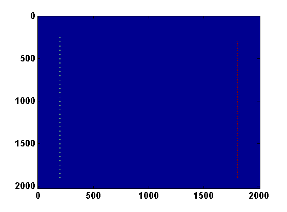
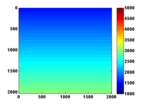
Consider a 2D synthetic experiment with a roughly \(200\) by \(200\) sized model and a mesh width \(h\) equal to \(10\) meters. The synthetic velocity model shown in Figure 3a has a constant high velocity region surrounded by a slower smooth background. We use an estimate of the smooth background as our initial guess \(m^0\). Similar to Example 1 in (T. van Leeuwen and Herrmann, 2013b), we put \(N_s = 39\) sources on the left and \(N_r = 96\) receivers on the right as shown in Figure 3b. The sources \(q_{sv}\) correspond to a Ricker wavelet with a peak frequency of \(30\)Hz.

Data is synthesized at \(18\) different frequencies ranging from \(3\) to \(20\) Hertz. Random Gaussian noise is added to the data \(d_v\) independently for each frequency index \(v\) and with standard deviations of \(\frac{.05 \|d_v\|}{\sqrt{N_s N_r}}\). This may not be a realistic noise model, but it can at least indicate that the method is robust to a small amount of noise in the data.

Two different choices for the regularization parameter \(\tau\) are considered: \(\tau = .875\tau_{\text{true}}\), where \(\tau_{\text{true}}\) is the total variation of the true slowness squared, and \(\tau = 1000\tau_{\text{true}}\), which is large enough so that the total variation constraint has no effect. Note that by using the Gauss Newton step from (\(\ref{bounds}\)) as an initial guess, the convex subproblem in (\(\ref{pTVb}\)) converges immediately in the large \(\tau\) case. The parameter \(\lambda\) for the PDE penalty is fixed at 1 for all experiments.

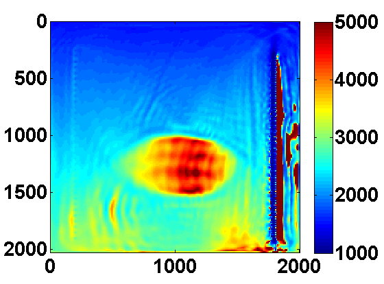
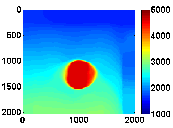
Results of the two experiments are shown in Figure 4. Including TV regularization reduced oscillations in the recovered model and led to better estimates of the high velocity region. Choosing \(\tau\) too large could make the TV constraint have no effect on the result, but there is also a risk of oversmoothing and completely missing small discontinuities when \(\tau\) is chosen to be too small.

Simultaneous Shot Example with Noise Free Data

Total variation regularization, in addition to making the inversion more robust to noise in he data, can also remove artifacts that arise when using few simultaneous shots. We consider a synthetic experiment with simultaneous shots where the true velocity model is a \(170\) by \(676\) 2D slice from the SEG/EAGE salt model shown in Figure 5a. A total of \(116\) sources and \(676\) receivers are placed near the surface, and a very good smooth initial model is used. We use frequencies between 3 and 33 Hz and the same frequency continuation strategy as before that works with overlapping batches of two.

The problem size is reduced by considering \(N_{ss} < N_s\) random mixtures of the sources \(q_{sv}\) defined by \[ \begin{equation} \bar{q}_{jv} = \sum_{s=1}^{N_s} w_{js}q_{sv} \qquad j = 1,...,N_{ss} \ , \label{simulshot} \end{equation} \] where the weights \(w_{js} \in \N(0,1)\) are drawn from a standard normal distribution. We modify the synthetic data according to \(\bar{d}_{jv} = P A_v^{-1}(m)\bar{q}_{jv}\) and use the same strategy to solve the smaller problem \[ \begin{equation} \begin{aligned} \min_{m,u} & \sum_{jv} \frac{1}{2}\|P u_{jv} - \bar{d}_{jv}\|^2 + \frac{\lambda^2}{2}\|A_v(m)u_{jv} - \bar{q}_{jv}\|^2 \\ & \text{s.t.} \qquad m_i \in [b_i , B_i] \text{ and } \|m\|_{TV} \leq \tau \ . \end{aligned} \label{altminss} \end{equation} \] Results using two simultaneous shots with no added noise and for two values of \(\tau\) are shown in Figure 6. With only two simultaneous shots the number of PDE solves is reduced by almost a factor of \(60\). TV regularization helps remove some of the artifacts caused by using so few simultaneous shots. In this case it mainly reduces noise under the salt and produces a smoother estimate of the salt body.

Benefit of Multiple Passes

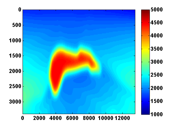
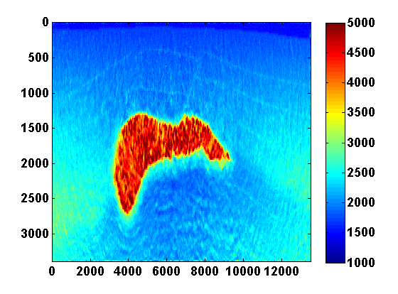
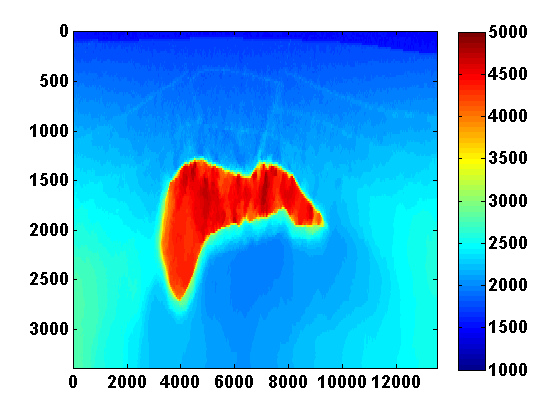
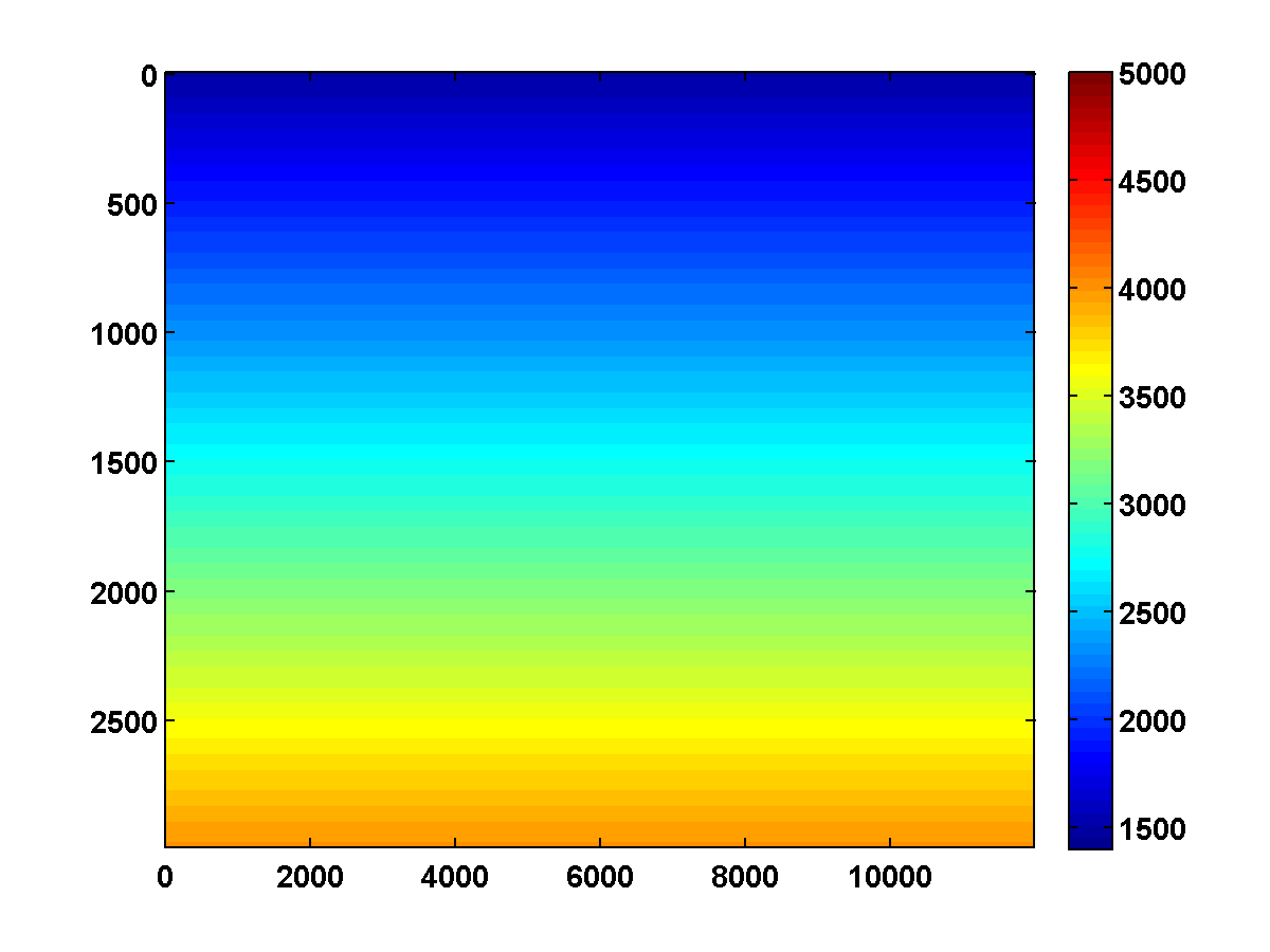
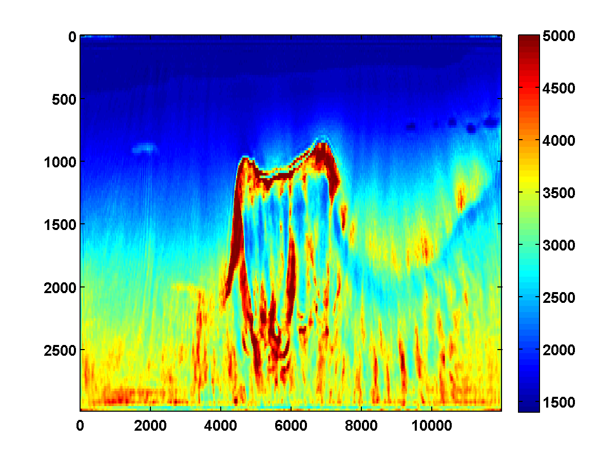
The results of the WRI method with frequency continuation can be improved by computing multiple passes through the frequencies, each time using the model estimated after the previous pass as a warm start [CITE BAS’S BG EXAMPLE]. The constrained WRI method also benefits from multiple passes. [INCLUDE SECOND PASS FOR PREVIOUS EXAMPLE] To illustrate this, consider the \(150\) by \(600\) model shown in Figure 7a, which corresponds to a downsampled upper left portion of the 2004 BP velocity benchmark data set (Billette and Brandsberg-Dahl, 2005). We will start with the smooth model shown in 7c and again loop through the frequencies ranging from \(3\) to \(20\) Hertz from low to high in overlapping batches of two. The bound constraints on the slowness squared are defined to correspond to minimum and maximum velocities of \(1400\) and \(5000\) m/s respectively. The \(\tau\) parameter for the TV constraint is chosen to be \(.9\) times the TV of the ground truth model. To reduce computation time, we again use two simultaneous shots, but now with new Gaussian weights \(w_{sj}\) redrawn every time the model is updated. The estimated model after computing \(25\) outer iterations per frequency batch is shown in Figure 8a. Using this as a warm start for a second pass through the frequency batches from low to high yields the improved result in Figure 8b.

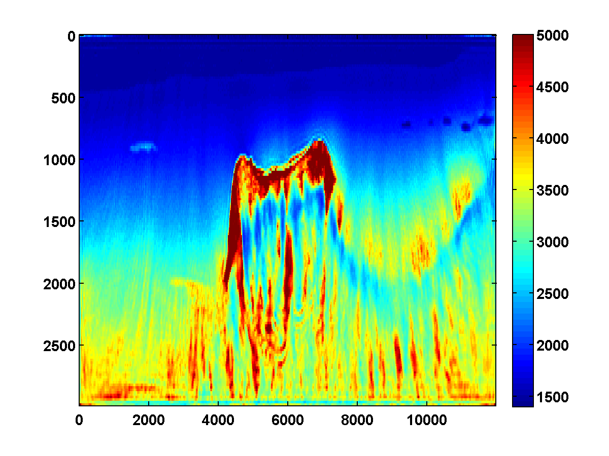
We run the same experiment using a weighted TV constraint with weights that decrease in depth as shown in Figure 9. The results shown in Figure 10 are similar, although some differences are apparent due to the weighted TV constraint being weaker in the deeper part of the model.

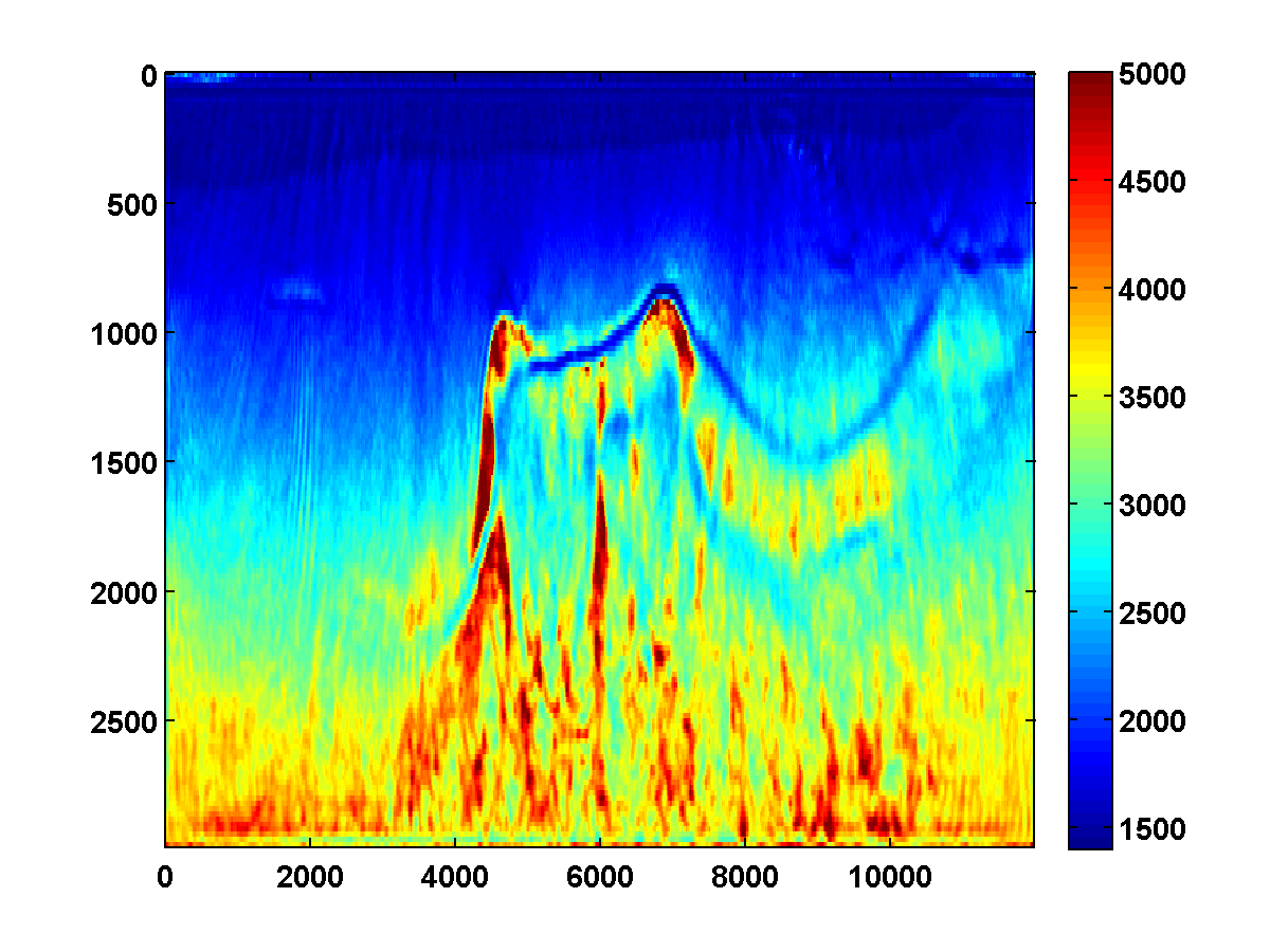
For comparison, two passes through the frequency batches are computed without any TV constraint, just the bound constraints. The results shown in Figure 11 appear much noisier. The estimated result after just one pass is notable because it has an oscillation just below the top of the salt on the left side. This mostly disappears after the second pass but isn’t present at all after one pass with either the TV or weighted TV constraints.

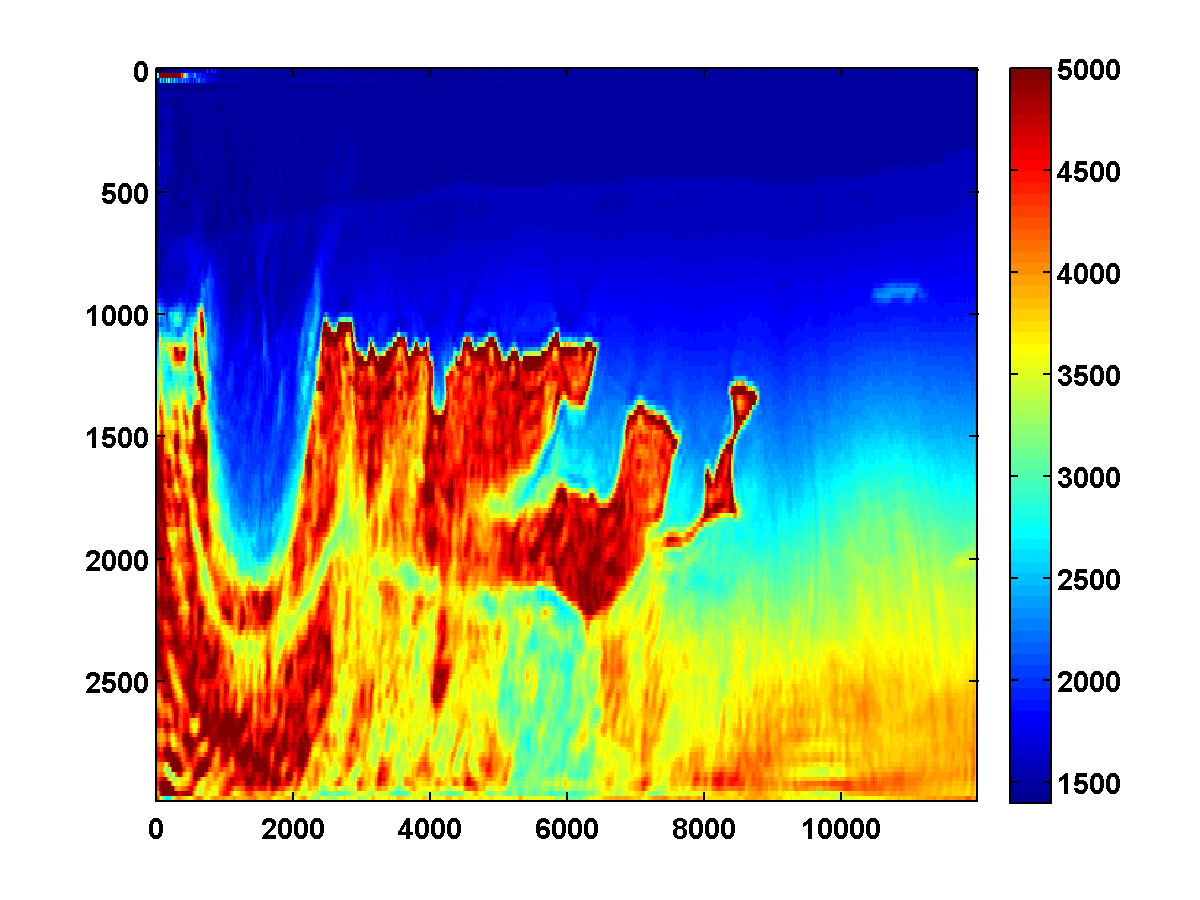
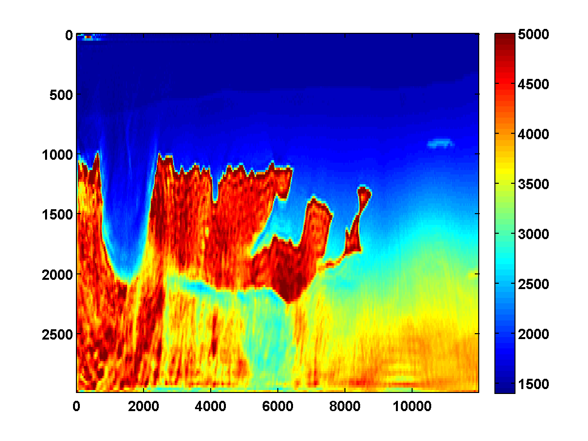
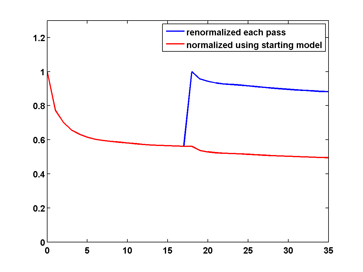
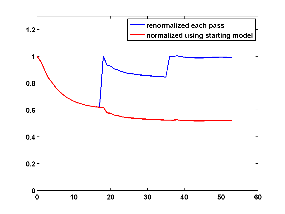
Figure 12 shows a comparison of the relative model errors defined by \(\frac{\|m - m_{\text{true}}\|}{\|m - m_{\text{init}}\|}\). The TV constrained examples both have lower model error than the unconstrained example.

One-Sided TV Constraint for Recovering Salt Bodies from Poor Initial Models

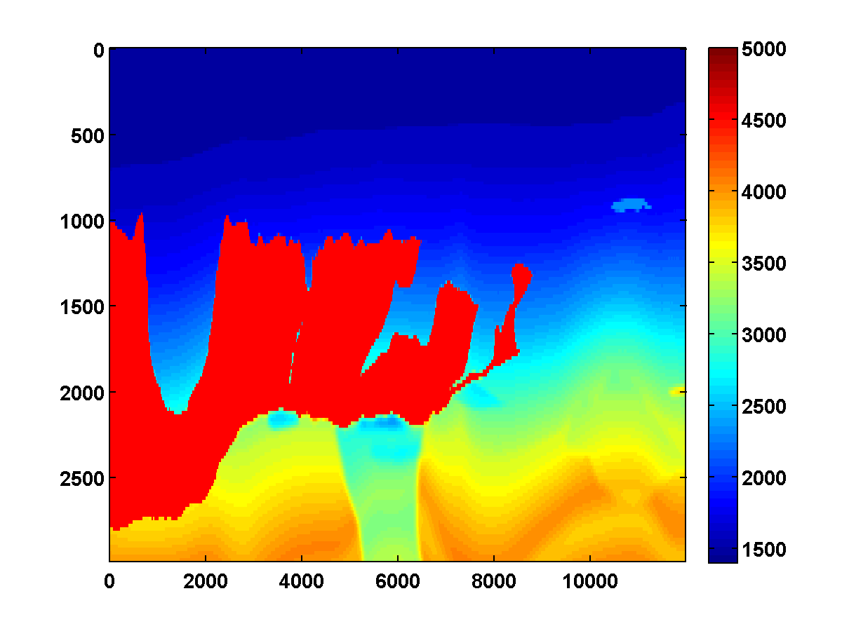
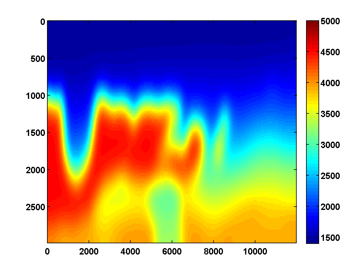
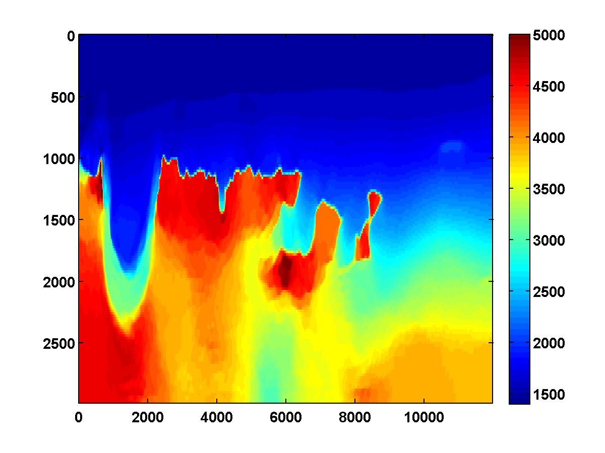
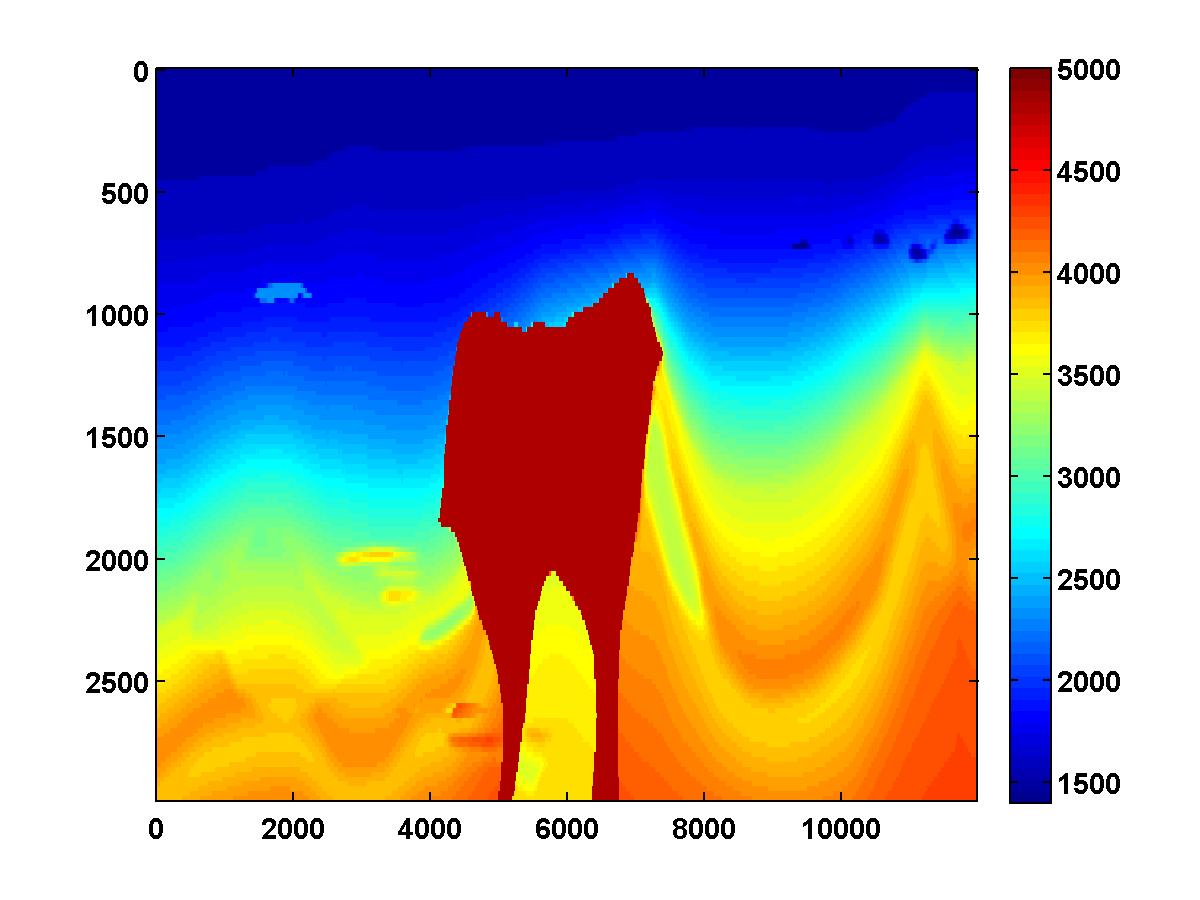
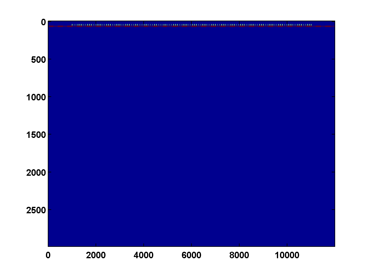
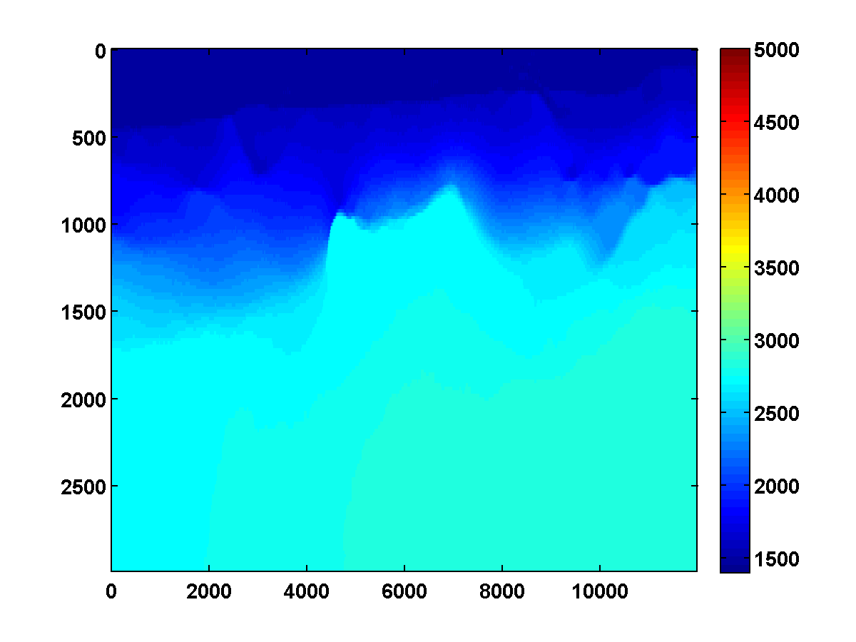
The inversion results shown in Figures 6b and 8b relied heavily on having good initial models, which for those examples were defined by smoothing the ground truth models. Consider the \(150\) by \(600\) velocity model shown in Figure 13a, which is the top middle portion of the same 2004 BP velocity benchmark data set, also downsampled. The same strategy that worked well for the top left portion of the model again works well if we initialize with a smoothed version of the true model. However, if we instead start with the poor initial model shown in Figure 13c, then the method appears to get stuck near a local minimum for which the inversion result is poor.

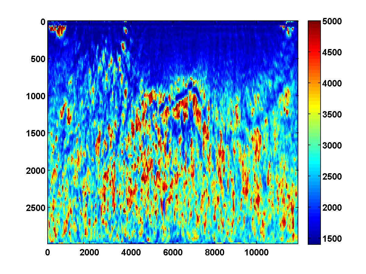
As shown in Figure 14, the WRI method with just bound constraints yields a very noisy result and fails to improve significantly even after multiple passes through the frequency batches.

With a TV constraint added, the method still tends to get stuck at a poor solution, even with multiple passes and different choices of \(\tau\). Figure 15 shows the estimated velocity models after three passes, where increasing values of \(\tau\) were used so that the TV constraint was weakened slightly after each pass.

Using a depth weighted TV constraint with the weights defined as in Figure 9 can slightly improve the solution because weights that decrease in depth prefer placing discontinuities in deeper parts of the model where the jumps are not as penalized, thus encouraging the lower boundary of the salt to move deeper as long at it continues to fit the data. The depth weighted TV result using Figure 15c as a starting model and \(\tau = .9 \tau_{\text{true}}\) is shown in Figure 16. While it’s an improvement, it doesn’t significantly update the initial model.

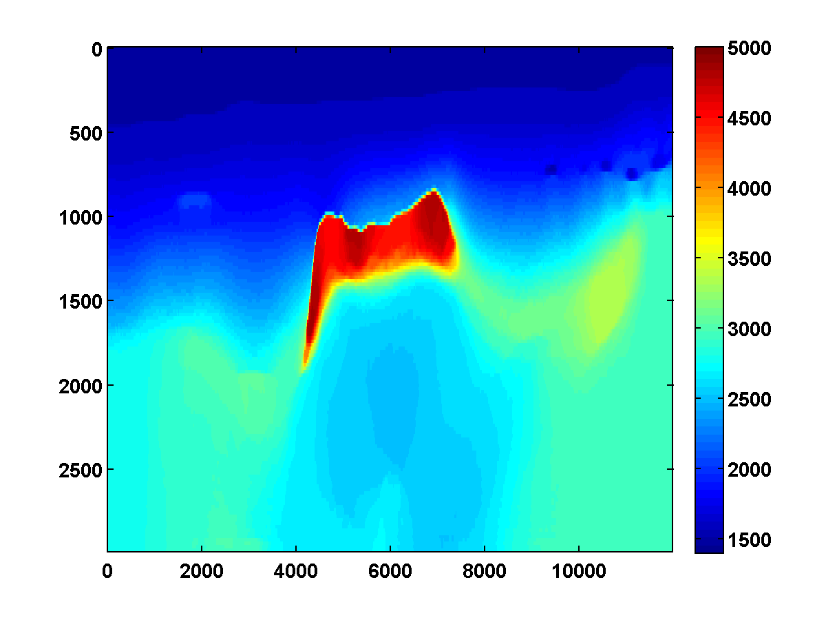
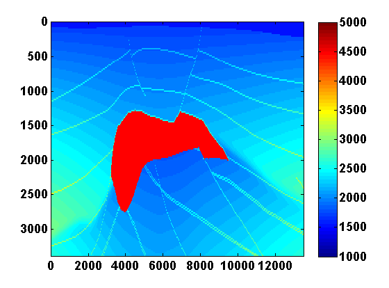
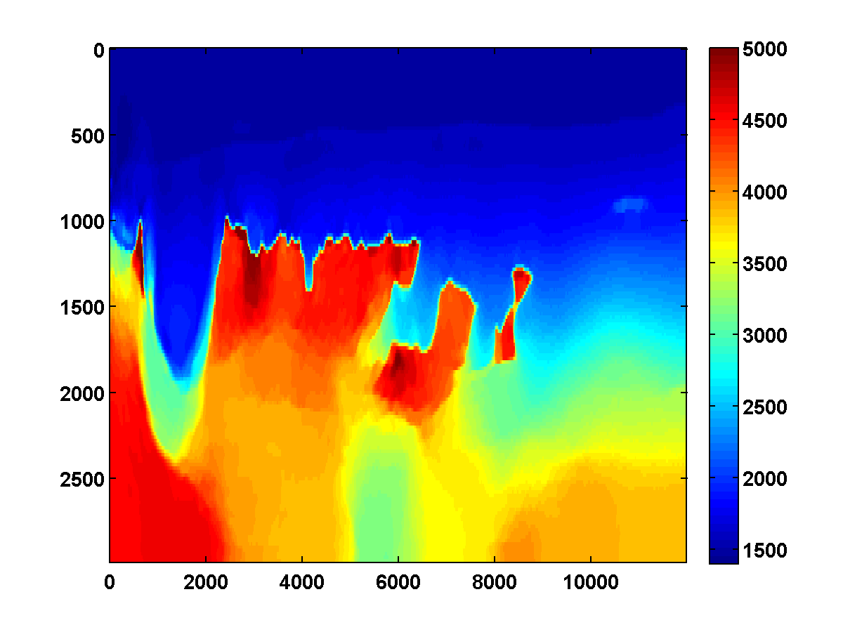
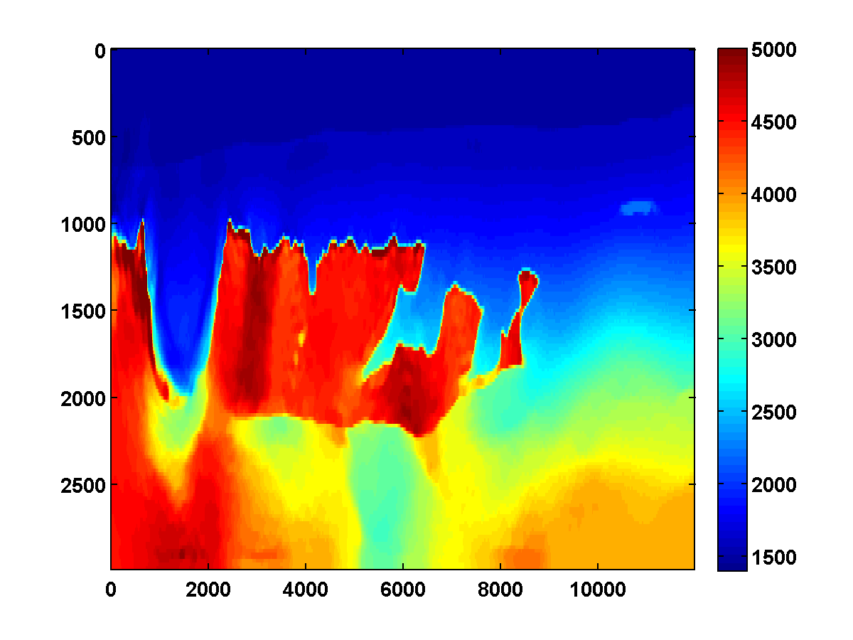
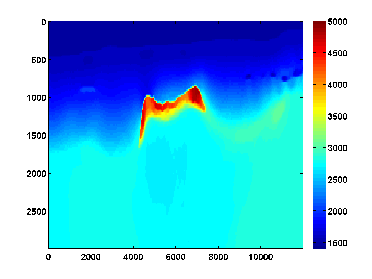
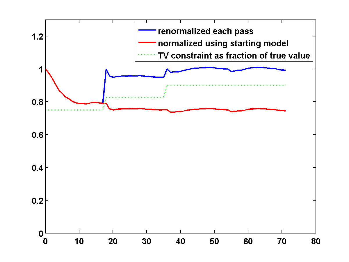
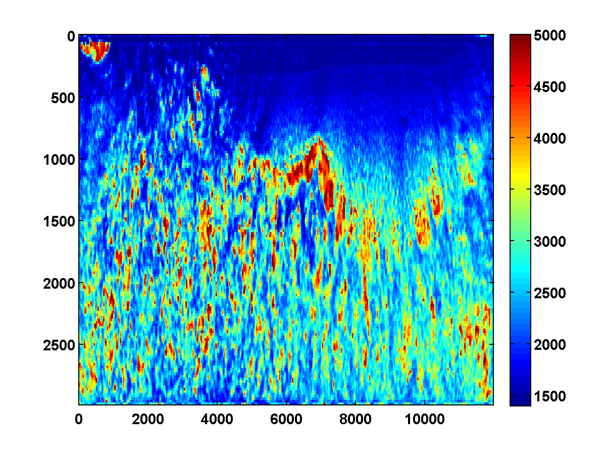
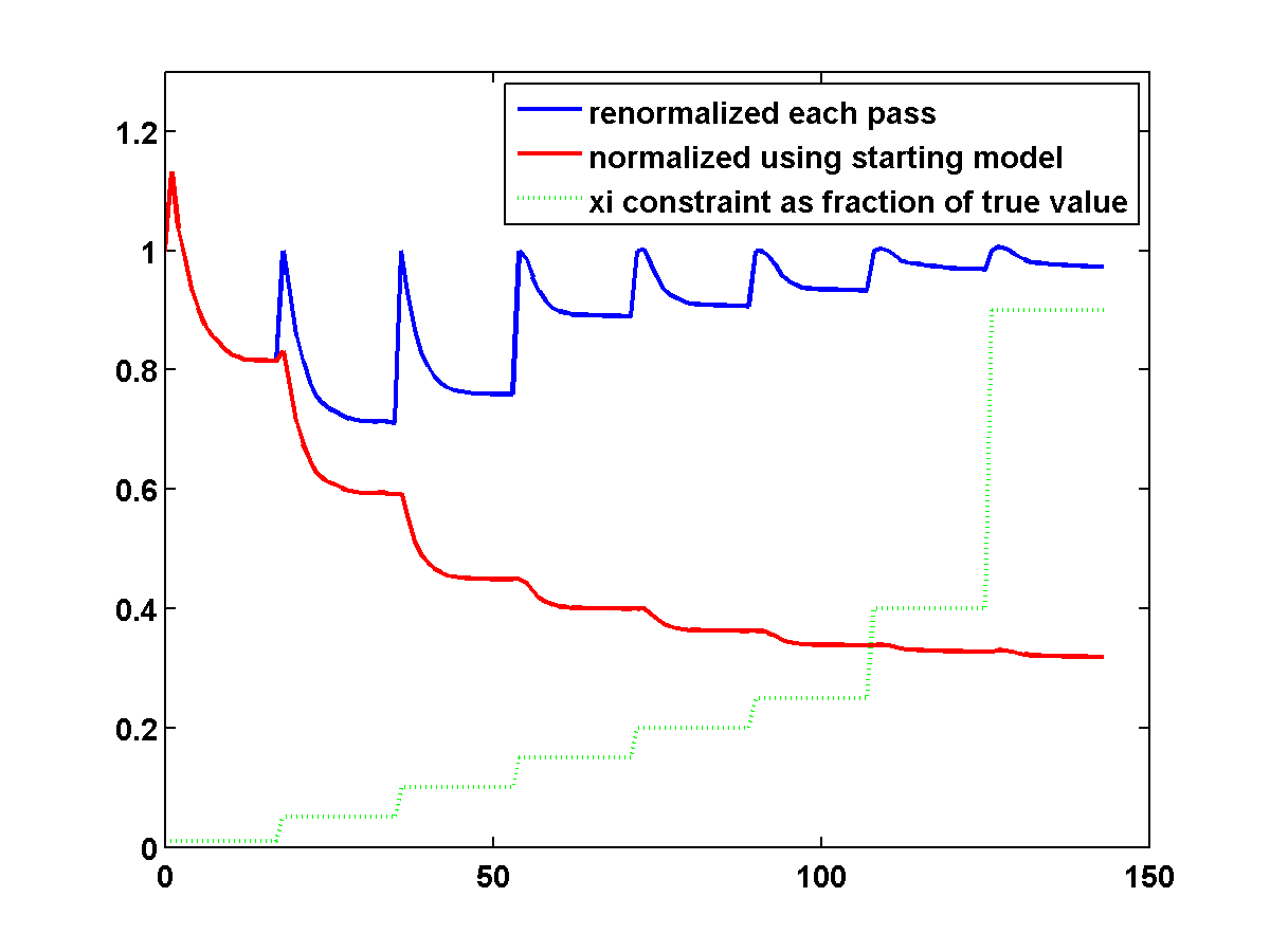
To discourage getting stuck in local minima that have spurious downward jumps in velocity, we consider adding the one-sided TV constraint and implementing a continuation strategy in the \(\xi\) parameter that starts with a small value and gradually increases it for each successive low to high pass through the frequency batches. This encourages the initial velocity estimate to be nearly monotonically increasing in depth. As \(\xi\) increases, more downward jumps are allowed. Again starting with the poor initial model in Figure 13c, Figure 17 shows the progression of velocity estimates over eight passes. The sequence of \(\xi\) parameters as a fraction of \(\|\max(0,D_z m_{\text{true}})\|_1\) is chosen to be \(\{.01, .05, .10, .15, .20, .25, .40, .90\}\). The \(\tau\) parameter is fixed at \(.9 \tau_{\text{true}}\) throughout. Although small values of \(\xi\) cause vertical artifacts, the continuation strategy is surprisingly effective at preventing the method from getting stuck at a poor solution. As \(\xi\) increases, more downward jumps in velocity are allowed, and the model error continues to significantly decrease during each pass.

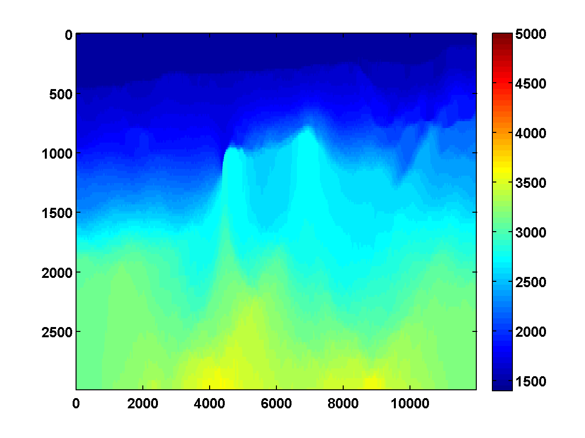
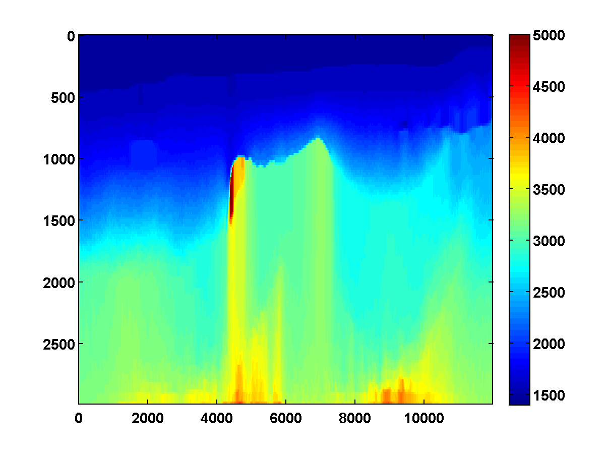
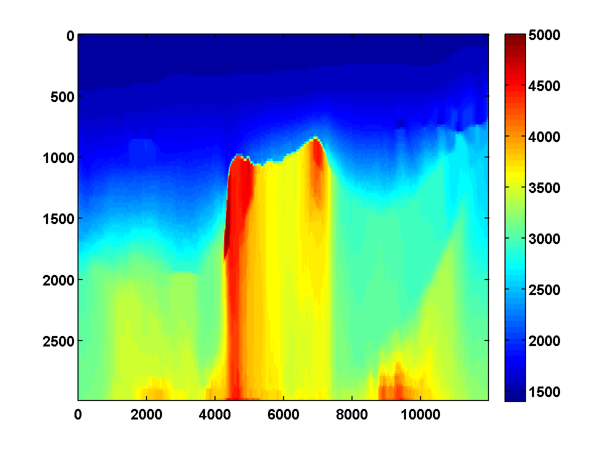
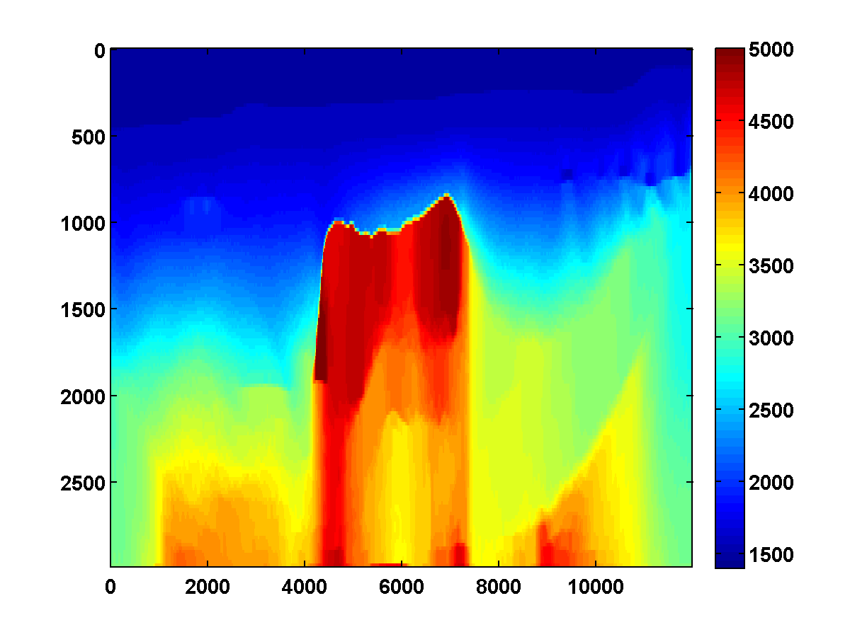
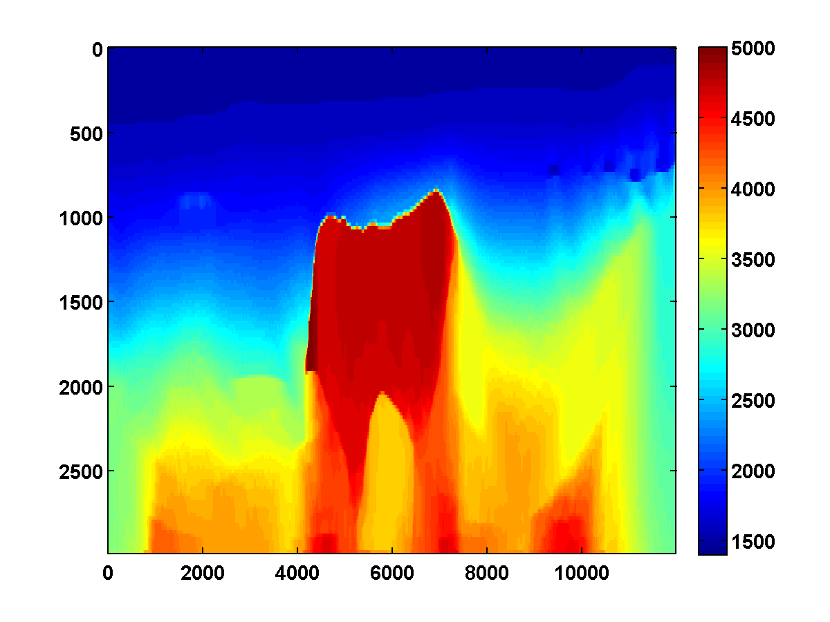
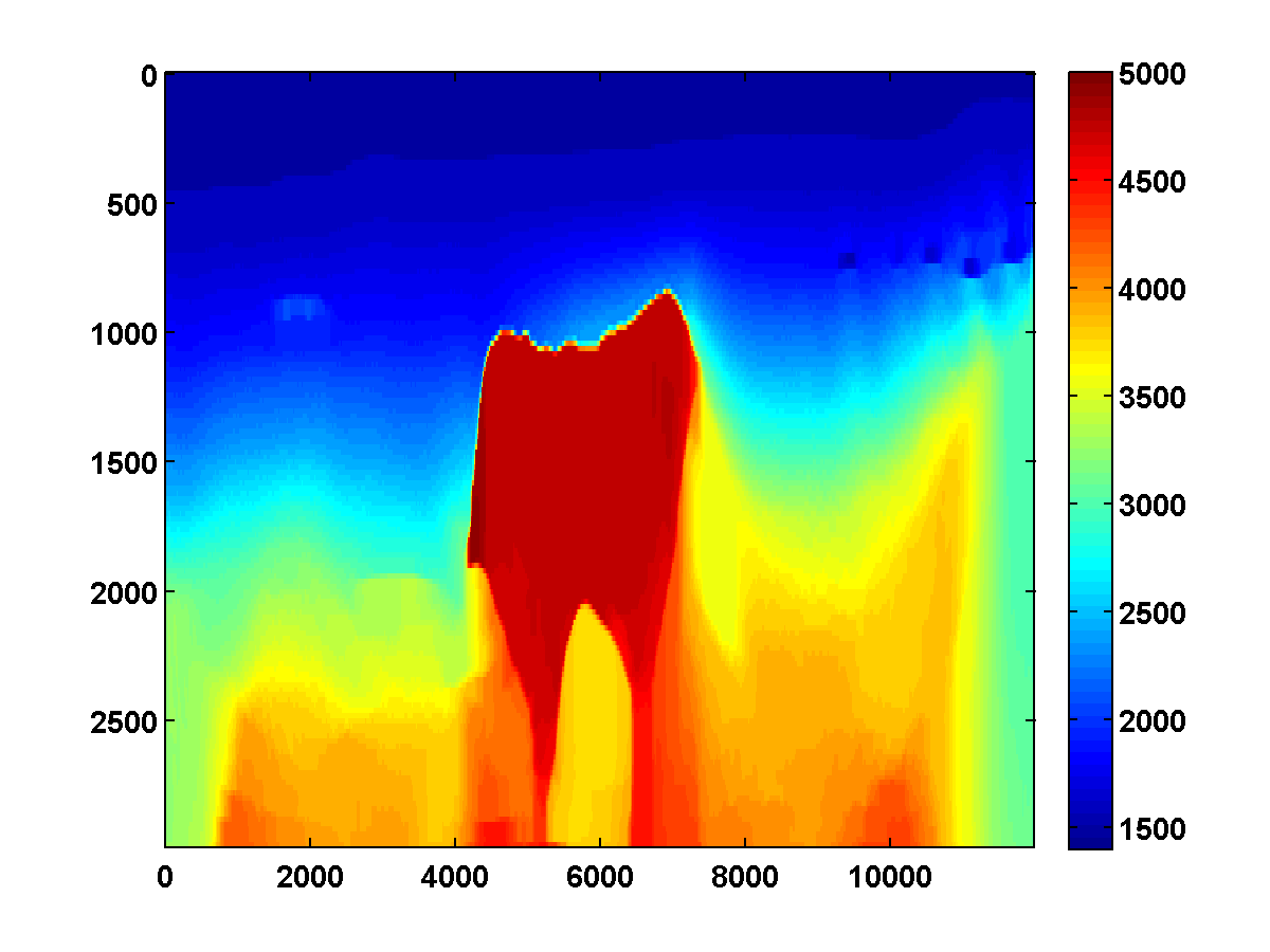
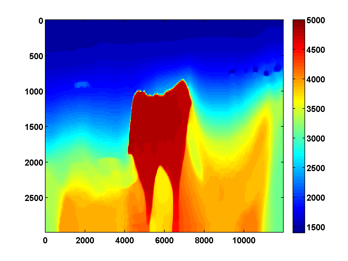
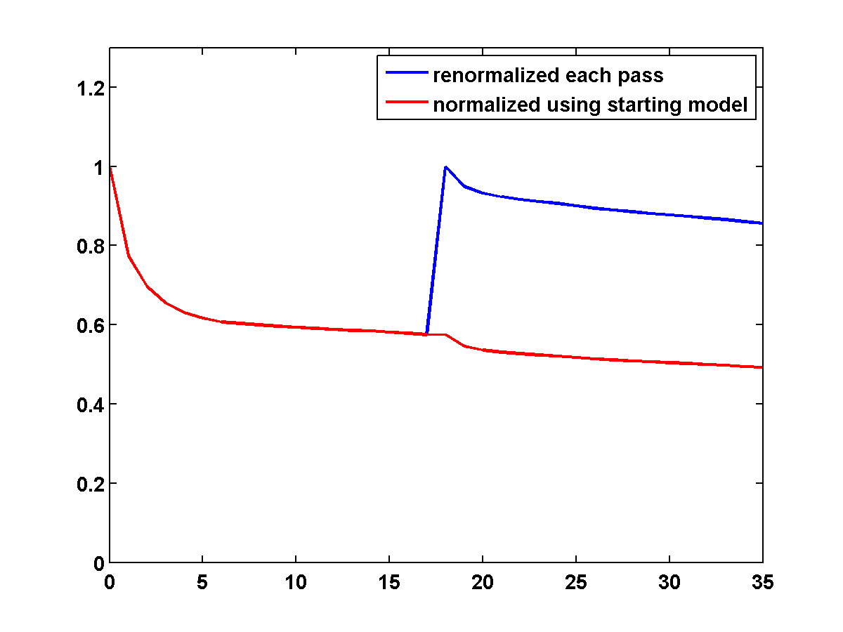
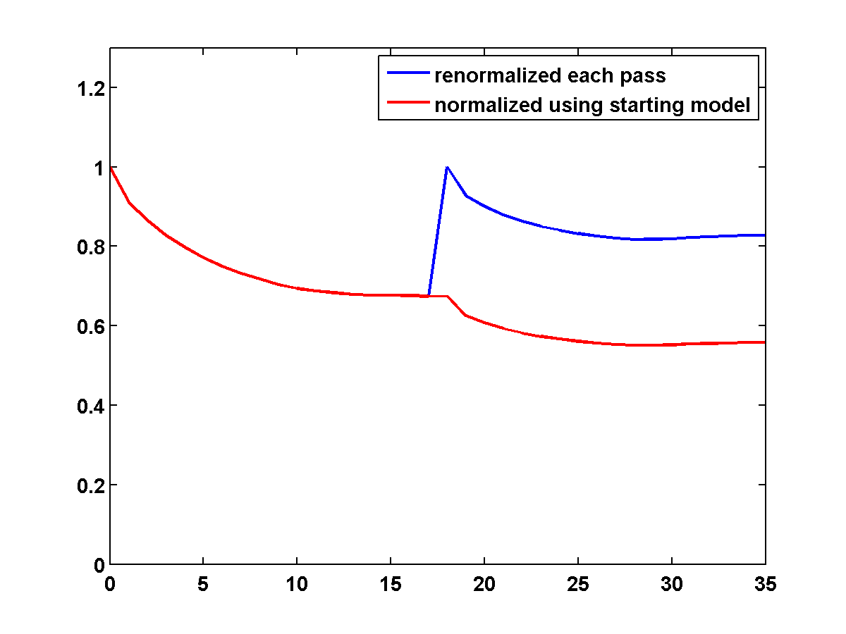
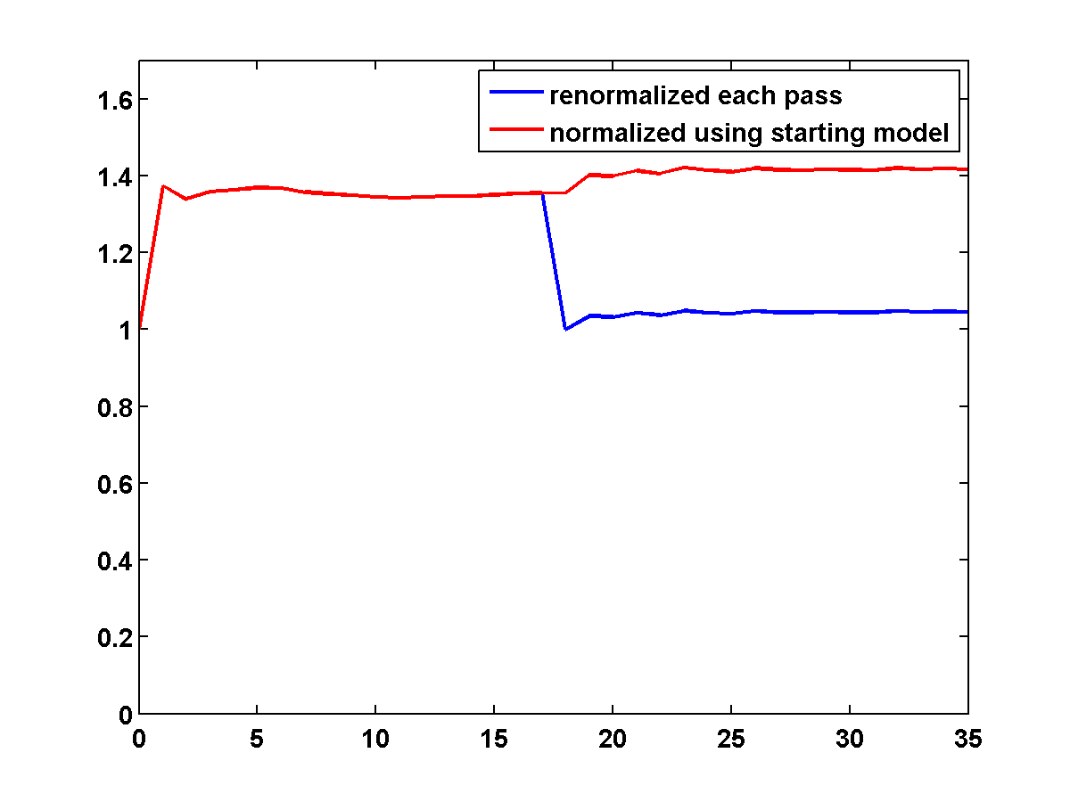
Figure 18 shows a comparison of the relative model errors for the previous three examples. Only the one-sided TV continuation results continue improving significantly after several passes.

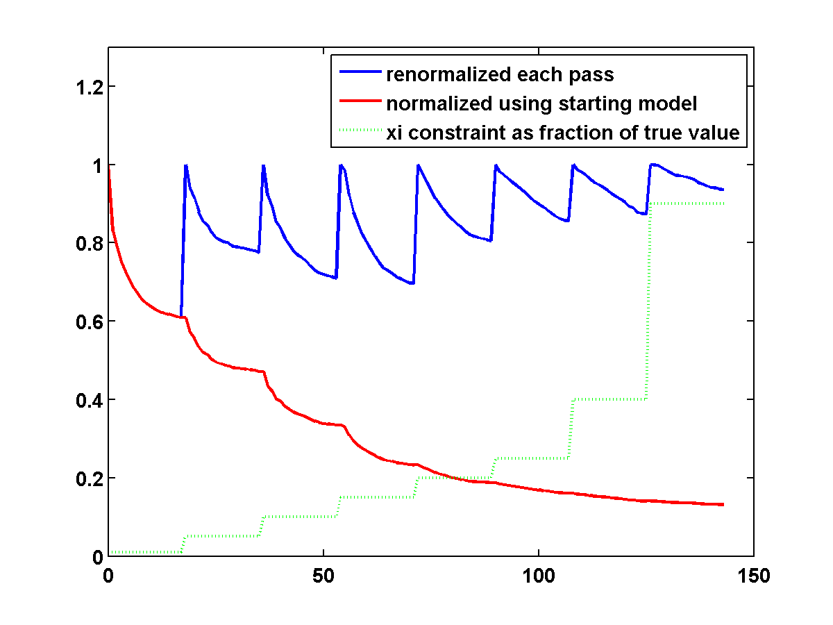
Even with a poor initial model, the one-sided TV constraint with continuation is able to recover the main features of the ground truth model. Poor recovery near the left and right boundaries is expected because the sources along the surface start about 1000m away from these boundaries.

Constrained Adjoint State Method Comparisons

The TV and one-sided TV constraints can also be used to improve the results of the adjoint state method. We still apply Algorithm 1 to the adjoint state formulation of (\(\ref{PDEcon2}\)), but with \(H^n + c_n\I\) replaced by \(c_n(H^n + \nu\I)\) where \(H^n\) is defined by (\(\ref{HAS}\)). Since this doesn’t approximate the Hessian as well as the Gauss Newton Hessian used in the quadratic penalty approach, some iterations are occasionally rejected as \(c_n\) is updated.

If we consider again the model in Figure 13a and start with the initial model in Figure 13c, the adjoint state methods with only bound constraints fails completely. The first update moves the model away from the ground truth, and the method quickly stagnates at the very poor result shown in Figure 19

On the other hand, if we include TV and one-sided TV constraints and use the same continuation strategy used to generate the results in Figure 17, the results are nearly as good. The constrained adjoint state results are shown in Figure 20. Compared to the constrained WRI method, the results are visually slightly worse near the top and sides of the model. Additionally, the model error doesn’t decrease as much, but it’s encouraging that it once again continues to decrease during each pass instead of stagnating at a poor solution. Continuation in the \(\xi\) parameter for the one-sided TV constraint appears to be a promising strategy for preventing both the constrained WRI and adjoint state methods from stagnating in a poor solution when starting from a bad initial model.

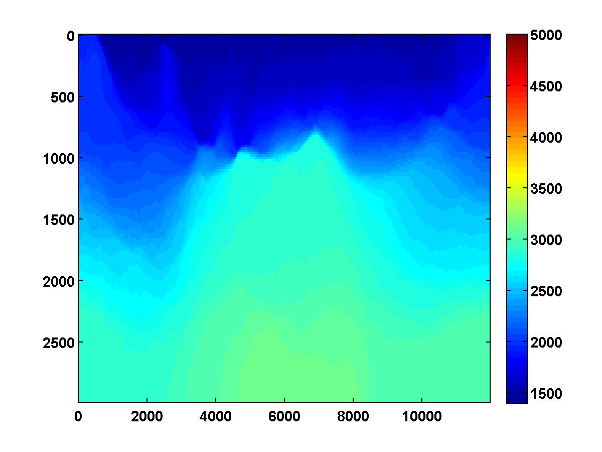
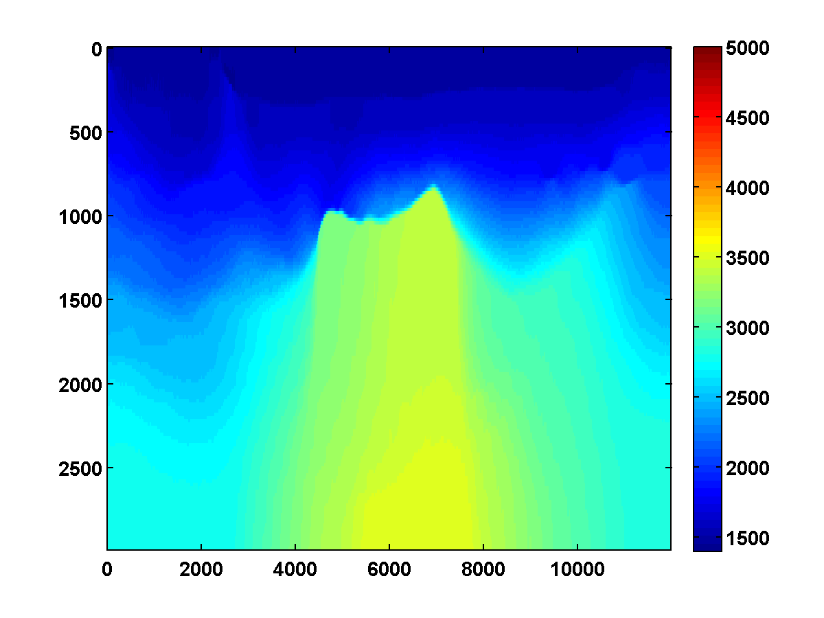
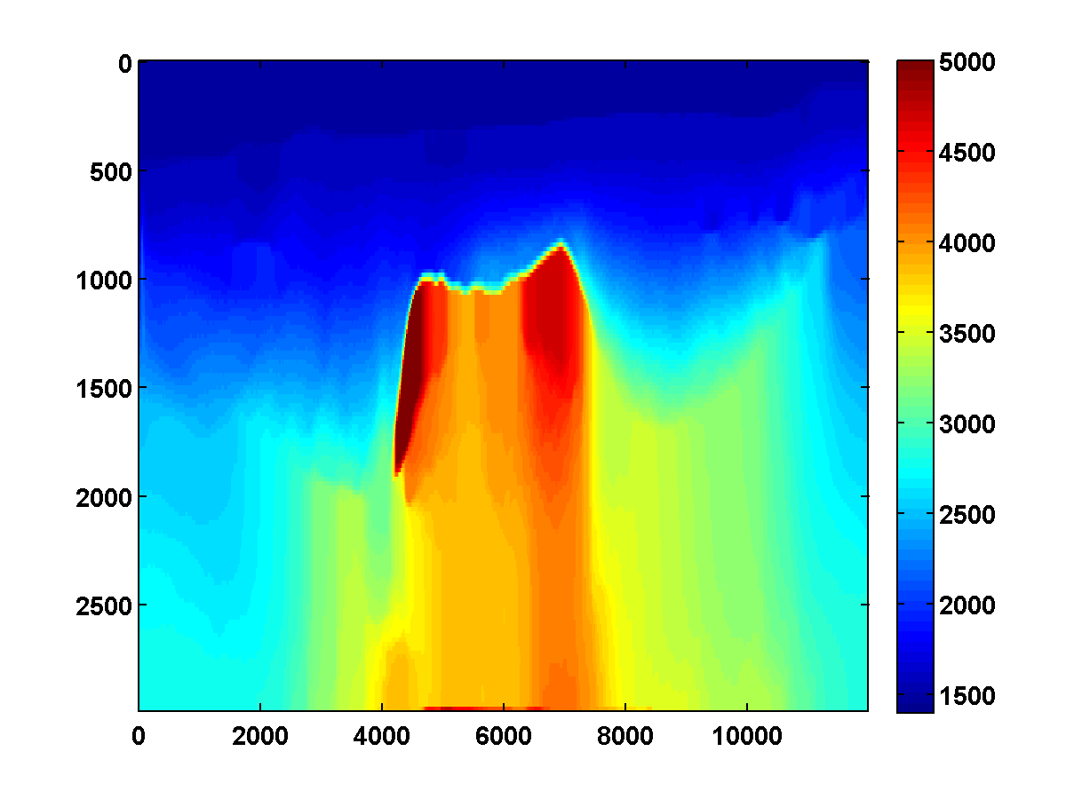
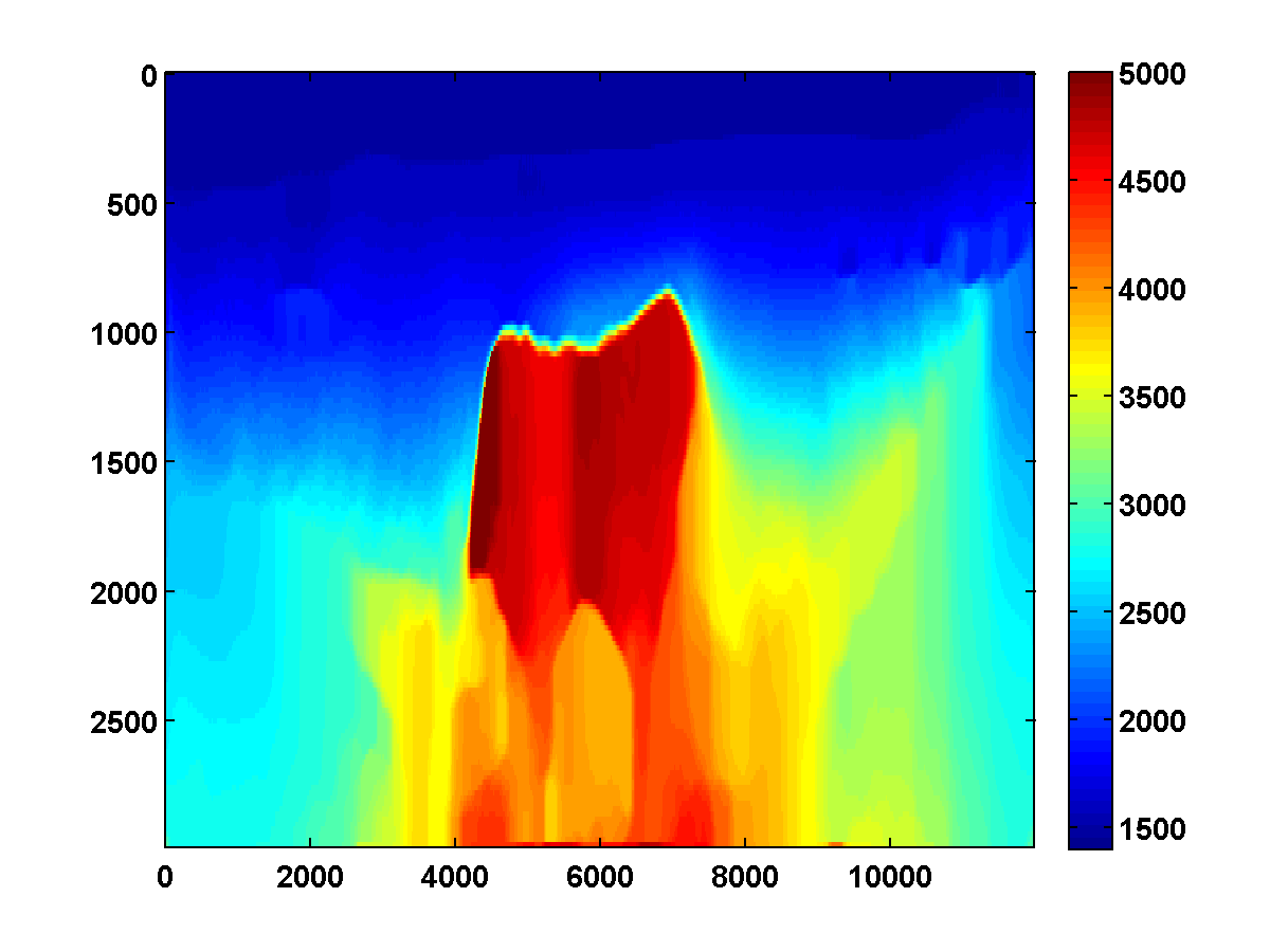
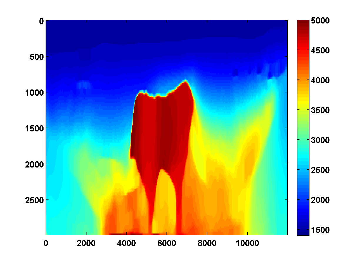
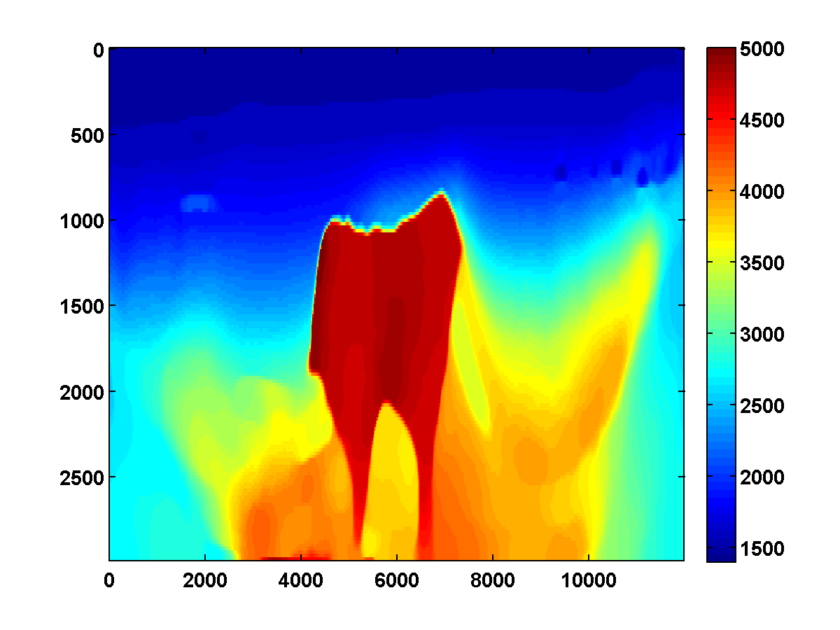
Figure 21 shows a comparison of the relative model errors for the previous two adjoint state examples. As in Figure 18 the one-sided TV continuation results continue improving significantly after several passes.

Ongoing Work

Many more experiments are required to answer lingering questions.

The numerical examples should be recomputed without inverse crime. Currently the same modeling operator was used both for inversion and for generating the synthetic data. In combination with the simplistic Robin boundary condition, this may conspire to make the inverse problem easier. However, the comparisons between methods and the relative benefits of the TV constraints are still meaningful. An interesting test would be to simply generate the data using more sophisticated modeling and boundary conditions while continuing to use the simple variants for inversion.

To remove any effect of randomness, the examples should be recomputed using sequential shots instead of simultaneous shots with the random weights redrawn every model update. This will be more computationally expensive, but it’s doable and is not expected to significantly alter the results.

The numerical examples using the one-sided TV continuation should be recomputed without the depth weighting. This is expected to have only a small effect on the results. It’s possible, however, that different parameter choices may be required.

It may be possible to improve the results shown in Figure 15 with different continuation strategies in the \(\tau\) parameter. Experiments that started with very small values of \(\tau\) were not initially promising, but so few experiments have been computed that the parameter selections are certainly not optimal.

More practical methods for selecting the parameters and more principled ways of choosing continuation strategies are needed. Currently the \(\tau\) and \(\xi\) parameters are chosen to be proportional to values corresponding to the true solution. Although the true solution clearly isn’t known in advance, it may still be reasonable base the parameter choices on estimates of its total variation (or one-sided TV). It would be even better to develop continuation strategies that don’t rely on any assumptions about the solution but that are still effective at regularizing early passes through the frequency batches to prevent the method from stagnating at poor solutions.

There is a lot of room for improvement in the algorithm used to solve the convex subproblems. There are for example methods such as the one in (Chambolle and Pock, 2011) that have better theoretical rates of convergence and are straightforward to implement.

It will be important to study how the method scales to larger problems. One effect is that the convex subproblems are likely to require more iterations. If they become too computationally expensive, then it may be better to replace the adaptive step size strategy in Algorithm 1 with a more standard line search. It would be good in any case to compare the efficiency of some other line search tecnhiques.

Continuation strategies that take advantage of the ability to enforce spatially varying bound constraints have still not been explored here. It should be possible for example to control what parts of the model are allowed to update. Other constraints can be considered that keep the updates closer to the initial model in places where it is more trusted.

If possible, it would also be good to experiment with different frequency continuation and sampling strategies as well as methods that attempt to minimize over all frequencies simultaneously.

Conclusions and Future Work

We presented a computationally feasible scaled gradient projection algorithm for minimizing the quadratic penalty formulation for full waveform inversion proposed in (T. van Leeuwen and Herrmann, 2013b) subject to additional convex constraints. We showed in particular how to solve the convex subproblems that arise when adding TV, one-sided TV and bound constraints on the model. The proposed framework is general, and the TV constraint can for instance be straightforwardly replaced by an \(l_1\) constraint on the curvelet coefficients of the model or combined with other convex constraints.

Synthetic experiments suggest that when there is noisy or limited data, TV regularization can improve the recovery by eliminating spurious artifacts. Experiments also show that a one-sided TV constraint that encourages velocity to increase with depth helps recover salt structures from poor initial models. In combination with a continuation strategy that gradually weakens the one-sided TV constraint, it can prevent the method from getting prematurely stuck at a bad solution when starting with a poor initialization.

In future work, we want to find a more practical way of selecting the regularization parameters \(\tau\) and \(\xi\) as well as more principled continuation strategies for adjusting them during multiple passes through frequency batches. It would be interesting if a numerical framework along the lines of the SPOR-SPG method in (Berg and Friedlander, 2011) could be extended to this application. Another direction we want to pursue is to consider nonconvex sparsity penalties on the gradient of the model, penalizing for instance the ratio of the \(l_1\) and \(l_2\) norms of the gradient. We also intend to study more realistic numerical experiments and investigate how to better take advantage of the proposed constrained WRI framework.

Acknowledgements

Thanks to Lluis Guasch [ASK TO ADD AS AUTHOR] for suggesting the 2004 BP dataset to better show the merits of the TV constrained WRI method and for designing the numerical examples shown in Figures 7 and 8. Thanks to Bas Peters for insights about the formulation and implementation of the penalty method for full waveform inversion including the strategies for frequency continuation and computing multiple passes with warm starts. Thanks also to Polina Zheglova for helpful discussions about the boundary conditions.