Full Waveform Inversion with Interferometric Measurements

Introduction

Full waveform inversion

Full waveform inversion in the frequency domain aims to construct high resolution seismic images by minimizing the misfit function \[ \begin{equation} \label{eq:1} \chi=\min \|F(m)-d\|_2, \end{equation} \] where \(F\) is the forward operator, \(m\) is the squared slowness, and \(d\) is the data. It is well recognized that suitable choice of misfit function is crucial for the recovery. There are many variations of the least-squares misfit function. For example, in time domain inversion, (Luo & Schuster, 1991) proposed to minimize the time difference of the observed and synthesis data which is reflected in their cross-correlation. (Fichtner, B.L. Kennett, H. Igel, & Bunge, 2009) used a time-frequency misfits to minimize both phase and envelop errors.

The least-squares solution of Eq. \(\ref{eq:1}\) seems unbeatable when nothing is assumed about the noise. In this note, we aim at designing misfit function to reduce the noise caused by two types of uncertainties.

• the displacement of the sources and receivers (e.g., the effects of statics)
• the inaccurate estimate of the background velocity

Under such noise, we will observe that

• in a common shot gather with closely located receivers, all the traces are shifting to the same direction and by a similar amount, or
• in a common receiver gather with closely located sources, all the traces are shifting to the same direction and by a similar amount.

This coherent shifting suggests a potential benefit of using interferometric measurements.

Interferometry

Seismic interferometry generally refers to the usage of the cross-correlation of two traces to fulfill inversion or imaging tasks.

Let \(u(x_s,x_r,t)\) be the full waveform that is sent from a source located at \(x_s\) and recorded by a receiver at \(x_r\), and let \(d(x_s,x_r,\omega) =\mathcal{F}(u)(x_s,x_r,\omega)\) be its Fourier transform along the time axis. Let \(n_s\) and \(n_r\) be the number of sources and receivers, and assume each pair is active. We store the \(n_s n_r\) traces in \(u_i(t)\), \(i=1,...,n_sn_r\), and the \(n_sn_r\) Fourier coefficients of them at a given frequency \(\omega\) in a vector \(d_\omega \in \mathbb{C}^{n_sn_r}\). Then the cross correlation of the traces in time domain corresponds to the outer product of the data in the frequency domain. \[ \begin{equation*} \mathcal{F}(u_i \star u_j )\equiv \mathcal{F}\left(\int \overline{u_i(s)} u_j(s+t)ds \right)=\overline{d_\omega(i)}d_\omega(j) \end{equation*} \] where \((a\star b)(t):=\int \overline{a(s)} b(t+s) ds\) with \(\bar a\) being the complex conjugate of \(a\), and \(\mathcal{F}\) denotes the Fourier transform.
Besides its original usage of reconstructing the impulse response of a given media, interferometry has recently found more applications in the seismic area. In particular, for both migration imaging (Borcea, G. Papanicolaou, & Tsogka, 2005) and inversion (Jugnon & Demanet, 2013), fitting the interferometric measurements \(d_\omega\) was used to enhance the robustness of the reconstructed image under modeling errors. Specifically, (Jugnon & Demanet, 2013) proposed the following misfit function for least-squares migration: \[ \begin{equation*} \begin{aligned} \hat{R}&=\arg \min\limits_{R}\|E\circ (\nabla\widetilde{F} R R^* \nabla\widetilde{F}^*-dd^*)\|_F^2 +\lambda\|R\|_F^2 \\ &\text{ subject to } \text{rank}(R)=K, \end{aligned} \end{equation*} \] where \(K\geq 2\) is some small integer less than the data dimension, \(d\) is the data which may contain one or more frequencies \(d=\{d_\omega, \omega\in \Omega\}\), \(d^*\) is the conjugate transpose of \(d\), \(\nabla\widetilde{F}\) is the Jacobian of the perturbed forward operator, and \(E\) is a restriction operator which selects a predefined subset of entries of \((\nabla\widetilde{F} R R^* \nabla\widetilde{F}^*-dd^*)\). The physical meaning is that for a given frequency, data from only some of the source-receiver combinations are used. The subset is chosen in a way that guarantees the maximal theoretical stability with respect to general additive noise.
The purpose of this note is to modify this idea for it to be extendable to nonlinear waveform inversion settings and explore its benefits.

Source or receiver displacement

Suppose either the sources or receivers have displacement but not both. Without loss of generality, we assume the uncertainty is on the source locations.
Let \(N=\{(i,j), i=1,...,n_s, j=1,…,n_r\}\) be the indices of all the source-receiver pairs and let \(P: N\rightarrow \mathbb{Z}_{n_sn_r}\) be a one to one map that vectorizes \(N\). Let \(\mathcal{E}_1^\epsilon \subseteq \mathbb{Z}_{n_sn_r}\times \mathbb{Z}_{n_sn_r} \) consists the indices of pairs of source-receiver pairs whose

• sources are the same
• receivers are \(\epsilon\)-close to each other.

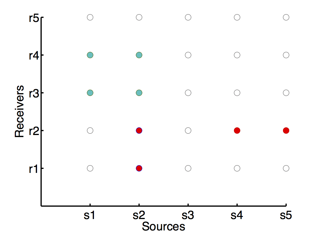
More specifically, let \(\left\{(i,j),(i',j')\right\}\) be a pair of source-receiver pair, then \(\{P(i,j),P(i',j')\} \in \mathcal{E}_1^\epsilon\), if \(x_{s_i}=x_{s_i'}\) and \(d(x_{r_j}, x_{r_j'})\leq \epsilon\) (see Fig. 3), where in the usual Euclidean space, we can take the distance \(d(\cdot,\cdot)\) to be the two norm \(\|\cdot\|_2\), and where \(x_{s_i}\) and \(x_{r_i}\) are the locations of the \(i\)th source and receiver. For the sake of simplicity, when there is no confusion, we write \(\mathcal{E}_1^\epsilon\) as \(\mathcal{E}_1\) for short.
We propose to replace the misfit function in Eq. \(\ref{eq:1}\) with \[ \begin{equation} \label{eq:s1} \min \|E\circ( \widetilde{F}(m)\widetilde{F}(m)^*-dd^*)\|_F \end{equation} \] for some \(E\subseteq \mathcal{E}_1^\epsilon\). Here \(\widetilde{F}\) denotes the forward operator corresponding to the presumed model while the true \(F\) that generated \(d=F(m)\) is unknown due to the source perturbation. When \(\epsilon=0\), we have \(\mathcal{E}_1^0=\{(i,i), i\in \mathbb{Z}_{n_sn_r}\}\), where we only try to fit the magnitude \(|d|\), which is exactly the phase retrieval problem. However, only fitting the magnitude may lead to non uniqueness of the solution. This can usually be avoided by increasing \(\epsilon\).

Theoretical motivation

A common understanding of the seismogram says that a relatively small change in the source or receiver location (comparing to the distance between the source and the receiver) will cause a time shift in the trace.
Fix a source \(s_0\) and two adjacent receivers \(x_{r_1}\) and x_{r_2}. Assume that when the source location \(x_s\) is accurate, the two traces are \(f(t)\) and \(g(t)\). When the location is inaccurate \(\widetilde{x_s}=x_s+\delta\), a phase shift will appear in the traces: \(\widetilde{f}(t)\approx f(t+ t_1)\) and \(\widetilde{g}(t)\approx g(t+ t_2)\). Since \(x_{r_1}\approx x_{r_2}\), we have \(t_1\approx t_2\). It is easy to see by that the cross correlation of \(f\) and \(g\) is then nearly unchanged \[ \begin{equation*} \mathcal{F}(f \star g) (\omega) \approx e^{i \omega(t_1-t_2)} \mathcal{F} (\widetilde{f}\star \widetilde{g})(\omega) \approx \mathcal{F}(\widetilde{f} \star \widetilde{g}) (\omega). \end{equation*} \] The equation implies that \(\mathcal{F}(f \star g)(w)\) as an element in \(dd^*\), is more robust that \(d\). This justifies why \(dd^*\) is a right quantity to be fitted.

Inaccurate background velocity

Inaccurate background velocity can cause similar effect in the trace as if there were source or receiver displacements. So we follow a similar logic as in the previous section except that the definition of \(\mathcal{E}_2^\epsilon\) is modified to include all the pairs of source-receiver pairs that have one of the following properties > 1. the pair have the same source and \(\epsilon\)-close receivers, > 2. the pair have the same receiver and \(\epsilon\)-close sources.

satisfies \[ \begin{equation} \label{eq:lift} \|\widetilde{F}(\hat{m})-e^{i\alpha} b\|\leq4\sqrt 2 \frac{\sqrt{\|\widetilde{F}\|^2+\|F\|^2}\|x\|^2\delta}{\sqrt{\lambda_2}} \end{equation} \] where \(\lambda_2\) is the second smallest eigenvalue of \(L_{|b|}\) and \(\alpha\) is some number in \([0,2\pi)\).

The theorem demonstrates how a small fitting error to the interferometric measurements leads to a small fitting error to the original data up to some global phase \(e^{i\alpha}\).

\(\textbf{Theorem 2.}\) Following our assumption in the previous section, that a small change in the source location will cause a time shift in the trace. In the frequency domain, this means the data has a large phase error and smaller magnitude error. This theorem deals with the extreme case of purely phase error, which is reflected in the assumption \(|\widetilde{F}(m)|=|b|\).

Trying to fit the outer product \(dd^*\) instead of \(d\) is called a ‘Phaselift’ by (Candés, Y. C. Eldar, Strohmer, & Voroninski, 2013). It is know that the Phaselift will cause a loss of global phase information. This can be seen by observing that two different vectors \(d\) and \(e^{\alpha i} d\) (\(\alpha\neq 0\)) are lifted to the same matrix \(dd^*=(e^{i \alpha } d)(e^{i \alpha } d)^*\). In order words, using only the lifted data, we cannot distinguish \(d\) and \(e^{\alpha i} d\). Therefore, to have any hope of recovering \(m\), it is necessary rule out those \(F\) that map another variable \(\tilde{m}\) to \(e^{i\alpha}F(m)\) with any \(\alpha\). This motivates the following definition.

\(\textbf{Definition 1.}\) Let \(F\) be an operator from \(\mathbb{C}^m\rightarrow \mathbb{C}^n\). Define \(D_x=\{e^{i\alpha} F(x), \alpha=[0,2\pi]\}\). If there exists a \(c>0\) such that \(c |x-y|\leq dist(D_x,D_y)\) for any \(x,y\in Domain(F)\), we call such an \(F\) a liftable operator with constant \(c\). Here for any closed sets \(A\), \(B\), we denote \(dist(A,B)=\min\limits_{x\in A, y\in B} \|x-y\|_2\).

For a forward operator \(F\) to be liftable, we need to place enough sources and receivers so that no two slowness models will produce seismograms that only differ by a global time delay. Once this is satisfied, the following theorem guarantees the reconstructions from Eq. #eq:p1 to be robust to modeling errors.

\(\textbf{Theorem 3.}\) Assuming the forward operator \(F\) is a liftable operator with constant \(c\), and \(\|F-\widetilde{F}\|\leq \delta <c\). Then the solution \(\hat{m}\) to Eq. satisfies \[ \begin{equation*} \|\hat{m}-m\|\leq 4\sqrt 2 \frac{\sqrt{\|\widetilde{F}\|^2+\|F\|^2}\|m\|^2\delta}{\sqrt \lambda_2(c-\delta)} +\frac{\delta\|m\|}{c-\delta} \end{equation*} \] where \(\delta\) and \(\lambda_2\) is the same as in Theorem 1.

High order interferometry

When both sources and receivers have displacements, the usual interferometric measurement \(dd^*\) is no longer a robust quantity. To deal with the increased uncertainty, we explore the fourth order cross correlation.
Assume there are four traces \(f_1(t),f_2(t),f_3(t),f_4(t)\). We define their cross correlation by \[ \begin{equation*} f_1\circ f_2\circ f_3\circ f_4:= (((f_1 \star f_2)\star f_3)\star f_4) \end{equation*} \] where \(\star \) is the cross correlation as defined in the first section. With this definition, we choose a set of certain quadruples as fitting indices. Specifically, for any fixed \(\epsilon\), the set \(\mathcal{E}_\epsilon \subseteq \mathbb{Z}_{n_sn_r}\times \mathbb{Z}_{n_sn_r}\times \mathbb{Z}_{n_sn_r}\times \mathbb{Z}_{n_sn_r}\) are defined by (see Fig. 3) \[ \begin{equation*} \begin{aligned} \mathcal{E}_3^\epsilon=&\{(P(i_1,j_1),P(i_2,j_2),P(i_3,j_3),P(i_4,j_4)), \\& x_{s_{i_1}}=x_{s_{i_2}},x_{s_{i_3}}=x_{s_{i_4}},x_{r_{j_1}}=x_{r_{j_3}}, x_{r_{j_2}}=x_{r_{j_4}} \\ & d(x_{s_{i_1}},x_{s_{i_3}})\leq \epsilon, d(x_{r_{j_1}},x_{r_{j_2}})\leq \epsilon \} \end{aligned} \end{equation*} \] Similar to above, we fit \[ \begin{equation} \label{eq:s2} \begin{aligned} \min & \|E_1\circ( \widetilde{F}(m)\widetilde{F}(m)^*-dd^*)\|_F^2\\ &+\|E_2 ( \widetilde{F}(m)\otimes \overline{\widetilde{F}(m)}\otimes \overline{\widetilde{F}^*(m)} \otimes \widetilde{F}(m)-d \otimes \overline d \otimes \overline d\otimes d)\|_V^2 \end{aligned} \end{equation} \] where \(E_1\in \mathcal{E}_1^0\) (defined in Section 2), \(E_2\in \mathcal{E}_3^\epsilon\), \(\otimes\) is the high order tensor product and \(\|A\|_V\) denote the \(l_2\) norm of \(vec(A)\), the vectorization of \(A\).

Rationale

Any quadruple in \(\mathcal{E}_3\) involves only two sources and two receivers and is actually the exhaustive combination of them (see Fig. 3). Suppose with accurate source-receiver locations, the four traces of of a quadruple in \(\mathcal{E}_3\) are \(f_1(t),f_2(t),f_3(t),f_4(t)\).
Now the perturbation of sources and receivers are added: \(\widetilde{x}_{r_i}=x_{s_i}+\delta_{s_i}\), \(\widetilde{x}_{r_1}=x_{r_1}+\delta_{r_i}\). The traces are then shifted to \[ \begin{equation*} \begin{aligned} &\widetilde{f}_1(t)\approx \widetilde{f}_1(t+t_{\delta_{s_1}}+t_{\delta_{r_1}}), &\widetilde{f}_2(t)\approx \widetilde{f}_1(t+t_{\delta_{s_1}}+t_{\delta_{r_2}}), \\ &\widetilde{f}_3(t)\approx \widetilde{f}_1(t+t_{\delta_{s_2}}+t_{\delta_{r_1}}), & \widetilde{f}_4(t)\approx \widetilde{f}_1(t+t_{\delta_{s_2}}+t_{\delta_{r_2}}), \end{aligned} \end{equation*} \] where \(t_{\delta_{s_i}}\) (\(t_{\delta_{r_i}}\)) denote the time delay caused by the displacement of the \(i\)’th sources (receivers). Noting that the fourth order correlation satisfies \[ \begin{equation*} \begin{aligned} &\mathcal{F}(f_2(t+t_2)\circ f_1(t+t_1)\circ f_3(t+t_3)\circ f_4 (t+t_4))(\omega) \\&=e^{i \omega (t_1-t_2-t_3+t_4)}\mathcal{F}(f_2(t)\circ f_1(t)\circ f_3(t)\circ f_4 (t))(\omega). \end{aligned} \end{equation*} \] We can use it to deduce that \[ \begin{equation} \label{eq:5} \begin{aligned} \mathcal{F}(\widetilde{f}_2(t) \circ \widetilde{f}_1(t)\circ \widetilde{f}_3(t)\circ \widetilde{f}_4 (t))& \approx \mathcal{F}(f_2(t)\circ f_1(t)\circ f_3(t)\circ f_4 (t)) \\ &= d_{k_1} \bar d_{k_2} \bar d_{k_3} d_{k_4}, \end{aligned} \end{equation} \] where for any \(i=1,2,3,4\), \(k_i\) is the index of the source-receiver pair that was used to obtain the trace \(f_i\).
Eq. \(\ref{eq:5}\) says that \(d_{k_1} \bar d_{k_2} \bar d_{k_3} d_{k_4}\) with \((k_1,k_2,k_3,k_4)\in \mathcal{E}_3^\epsilon\) is a more robust variable than \(d\) under the source-receiver displacements.

Numerical Illustration

We test our algorithm on the constant velocity synthetic model.

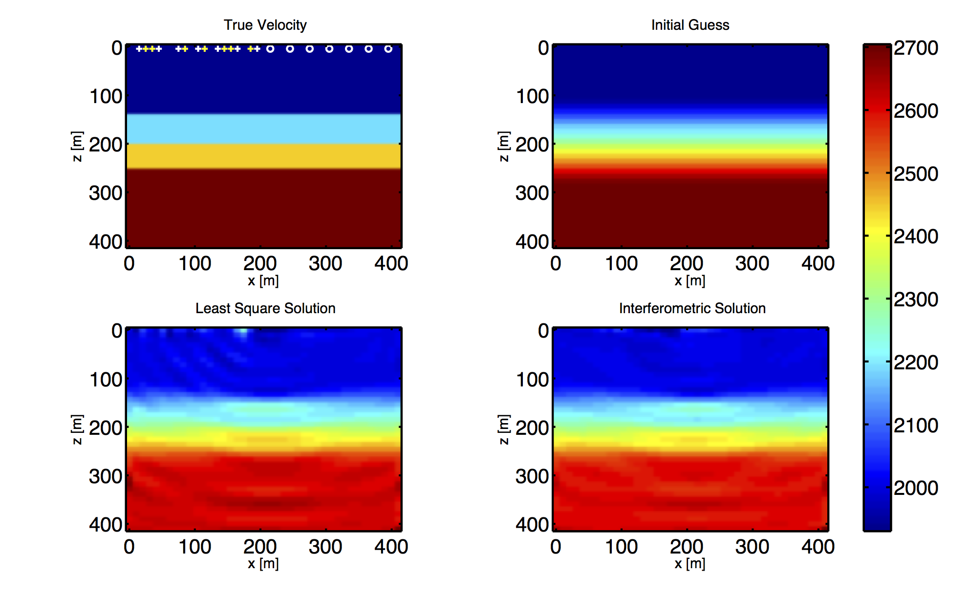
In the first experiment, we assume the modeling error is on the perturbation of the sources. The white pluses in the upper left image of Fig. 1 are the intended positions of the sources while the yellow pluses are their true locations. The white circles are both the intended and true positions of the receivers. We assume the perturbations are horizontal and uniformly distributed from -4 to 4 meters. The interferometric solution is obtained by solving Eq. \(\ref{eq:s1}\) with \(E\) chosen to be \[ \begin{equation*} \begin{aligned} E=& \{\left(P(i,i), P(i,j)\right),i=1,...,n_s, r_i \text{ and }r_j \text{ are neighbours}\} \\ &\cup \{(P(i,i), P(i,i)),i=1,...,n_s\} \}. \end{aligned} \end{equation*} \] From Fig. 1, we observe that the source perturbation generates a weak interference wave on the left half of the image of the least-squares solution, while the interferometric solver does a good job to avoid it.

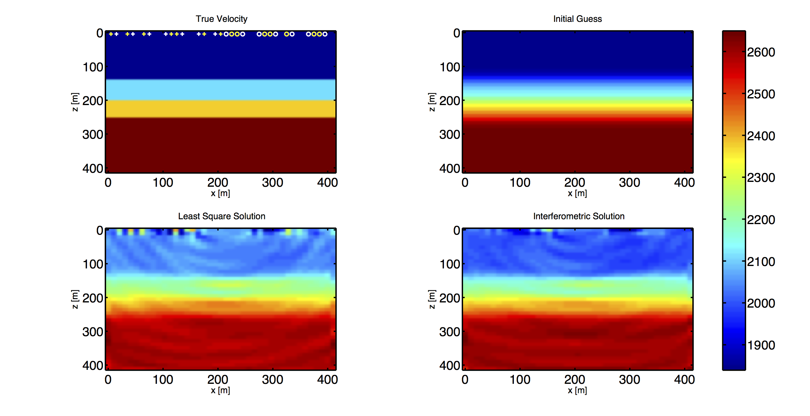
In the second experiment, we assume both sources and receivers have displacements. Each displacement is horizontal, independent, and uniformly distributed between -4m to 4m. We obtain the interferometric solution by minimizing Eq.\(\ref{eq:s2}\) with \(E_1\) and \(E_2\) defined by \[ \begin{equation*} \begin{aligned} E_1=& \{(P(i,i), P(i,i)),i=1,…,n_s\}, \\ E_2=& \{\left(P(i,i), P(i,j), P(i,k) \right),i=1,...,n_s, \\ & r_i, r_j \text{ and }r_k \text{ are neighbours}\}. \end{aligned} \end{equation*} \] Again, we find that the interferometric solution is more robust than the least-squares one.

Discussion and conclusions

We proposed several alternatives to the least-squares misfit function to increase robustness of the full waveform inversion under certain types of modeling errors. Theoretical bound on reconstruction errors of the interferometric fittings is established, which allows us to predict the quality of the final image.
We also introduced a high order interferometry to further increase the robustness when the uncertainty lies in both sources and receivers. As the first step, we only include the neighbouring points into the fitting indices (as in Fig. 3 ) in the simulation. A more careful way to do this is to include more points but with less weight if two points are farther away. This will certainly be a future research direction.

Acknowledgments

This work was partly supported by the NSERC of Canada Discovery Grant (22R81254) and the Collaborative Research and Development Grant DNOISE II (375142-08). This research was carried out as part of the SINBAD II project with support from BG Group, BGP, BP, Chevron, ConocoPhillips, Petrobras, PGS, Total SA, Woodside, Ion, CGG, Statoil and WesternGeco.

References

Borcea, L., G. Papanicolaou, & Tsogka, C. (2005). Interferometric array imaging in clutter. Inverse Problems, 21, 1419.
Candés, E. J., Y. C. Eldar, Strohmer, T., & Voroninski, V. (2013). Phase retrieval via matrix completion. SIAM Journal on Imaging Sciences, 6(1), 199–225.
Fichtner, A., B.L. Kennett, H. Igel, & Bunge, H. P. (2009). Full seismic waveform tomography for upper-mantle structure in the australasian region using adjoint methods. Geophysical Journal International, 179, 1703–1725.
Jugnon, V., & Demanet, L. (2013). Interferometric inversion: a robust approach to linear inverse problems. Proceedings of SEG Annual Meeting.
Luo, Y., & Schuster, G. T. (1991). Wave-equation traveltime inversion. Geophysics, 56, 645–653.