A scaled gradient projection method for total variation regularized full waveform inversion

Introduction

Acoustic full waveform inversion in the frequency domain can be written as the following PDE constrained optimization problem (F. J. Herrmann et al., 2013; Tarantola, 1984; Virieux & Operto, 2009) \[ \begin{equation} \label{PDEcon} \min_{m,u} \sum_{sv} \frac{1}{2}\|P u_{sv} - d_{sv}\|^2 \ \ \text{such that} \ \ A_v(m)u_{sv} = q_{sv} \ , \end{equation} \] where \(A_v(m)u_{sv} = q_{sv}\) denotes the discretized Helmholtz equation. Let \(s = 1,...,N_s\) index the sources and \(v = 1,...,N_v\) index frequencies. We consider the model, \(m\), which corresponds to the reciprocal of the velocity squared, to be a real vector \(m \in \R^{N}\), where \(N\) is the number of points in the spatial discretization. For each source and frequency the wavefields, sources and observed data are denoted by \(u_{sv} \in \C^N\),\(q_{sv} \in \C^N\) and \(d_{sv} \in \C^{N_r}\) respectively, where \(N_r\) is the number of receivers. \(P\) is the operator that projects the wavefields onto the receiver locations. The Helmholtz operator has the form \[ \begin{equation} \label{Helmholtz} A_v(m) = \omega_v^2 \diag(m) + L \ , \end{equation} \] where \(\omega_v\) is angular frequency and \(L\) is a discrete Laplacian.

The nonconvex constraint and large number of unknowns make (\(\ref{PDEcon}\)) a very challenging inverse problem. Since it is not practical to store all the wavefields, and it also is not always desirable to exactly enforce the PDE constraint, it was proposed in (T. van Leeuwen & Herrmann, 2013b, 2013a) to work with a quadratic penalty formulation of (\(\ref{PDEcon}\)), formally written as \[ \begin{equation} \label{penalty_formal} \min_{m,u} \sum_{sv} \frac{1}{2}\|P u_{sv} - d_{sv}\|^2 + \frac{\lambda^2}{2}\|A_v(m)u_{sv} - q_{sv}\|^2 \ . \end{equation} \] This is formal in the sense that a slight modification is needed to properly incorporate boundary conditions, and this modification also depends on the particular discretization used for \(L\). As discussed in (T. van Leeuwen & Herrmann, 2013b), methods for solving the penalty formulation seem less prone to getting stuck in local minima when compared to solving formulations that require the PDE constraint to be satisfied exactly. The unconstrained problem is easier to solve numerically, with alternating minimization as well as Newton-like strategies being directly applicable. Moreover, since the wavefields are decoupled it isn’t necessary to store them all simultaneously when using alternating minimization approaches.

The most natural alternating minimization strategy is to iteratively solve the data augmented wave equation \[ \begin{equation} \label{ubar} \bar{u}_{sv}(m^n) = \arg \min_{u_{sv}} \frac{1}{2}\|Pu_{sv} - d_{sv}\|^2 + \frac{\lambda^2}{2}\|A_v(m^n)u_{sv} - q_{sv}\|^2 \end{equation} \] and then compute \(m^{n+1}\) according to \[ \begin{equation} \label{m_altmin} m^{n+1} = \arg \min_m \sum_{sv} \frac{\lambda^2}{2}\|L\bar{u}_{sv}(m^n) + \omega_v^2 \diag(\bar{u}_{sv}(m^n))m - q_{sv}\|^2 \ . \end{equation} \] This can be interpreted as a Gauss Newton method for minimizing \(G(m) = \sum_{sv}G_{sv}(m)\), where \[ \begin{equation} \label{Gsv} G_{sv}(m) = \frac{1}{2}\|P \bar{u}_{sv}(m) - d_{sv}\|^2 + \frac{\lambda^2}{2}\|A_v(m)\bar{u}_{sv}(m) - q_{sv}\|^2 \ . \end{equation} \] Using a variable projection argument (Aravkin & Leeuwen, 2012), the gradient of \(G\) at \(m^n\) can be computed by \[ \begin{equation} \label{gradG} \begin{aligned} \nabla G(m^n) & = \sum_{sv} \re\left( \lambda^2 \omega_v^2 \diag(\bar{u}_{sv}(m^n))^* \right.\\ & \left. (\omega_v^2 \diag(\bar{u}_{sv}(m^n))m^n + L\bar{u}_{sv}(m^n) - q_{sv})\right) \ . \end{aligned} \end{equation} \] A scaled gradient descent approach (Bertsekas, 1999) for minimizing \(G\) can be written as \[ \begin{equation} \label{SGD} \begin{aligned} \dm & = \arg \min_{\dm \in R^N} \sum_{sv} \dm^T \nabla G_{sv}(m^n) + \frac{1}{2}\dm^T H_{sv}^n \dm \\ & \qquad \qquad \qquad + c_n \dm^T\dm \\ m^{n+1} & = m^n + \dm \ , \end{aligned} \end{equation} \] where \(H_{sv}^n\) should be an approximation to the Hessian of \(G_{sv}\) and \(c_n \geq 0\). Note that this general form includes gradient descent in the case when \(H=0\) and Newton’s method when \(H\) is the true Hessian and \(c=0\). In (T. van Leeuwen & Herrmann, 2013b), a Gauss Newton approximation is used, where \(c_n = 0\) and \[ \begin{equation} \label{H} H_{sv}^n = \re (\lambda^2 \omega_v^4 \diag(\bar{u}_{sv}(m^n))^*\diag(\bar{u}_{sv}(m^n)) \ . \end{equation} \] Since the Gauss Newton Hessian approximation is diagonal, it can be incorporated into (\(\ref{SGD}\)) with essentially no additional computational expense. This corresponds to the alternating procedure of iterating (\(\ref{ubar}\)) and (\(\ref{m_altmin}\)) at least for the formal objective that is linear in \(m\), which it may not be in practice depending on how the boundary conditions are implemented.

Including Convex Constraints

To make the inverse problem more well posed we can add the constraint \(m \in C\), where \(C\) is a convex set. For example, a box constraint on the elements of \(m\) could be imposed by setting \(C = \{m : m \in [B_1 , B_2]\}\). The only modification of (\(\ref{SGD}\)) is to replace the \(\dm\) update by \[ \begin{equation} \label{dmcon} \begin{aligned} \dm & = \arg \min_{\dm \in R^N} \sum_{sv} \dm^T \nabla G_{sv}(m^n) + \frac{1}{2}\dm^T H_{sv}^n \dm \\ & \qquad \qquad \qquad + c_n \dm^T\dm \ \text{ such that }\ m^n + \dm \in C \ . \end{aligned} \end{equation} \] This ensures \(m^{n+1} \in C\) but makes \(\dm\) more difficult to compute. The problem is still tractable if \(C\) is easy to project onto or can be written as an intersection of convex constraints that are each easy to project onto. This convex subproblem is unlikely to be a computational bottleneck relative to the expense of solving for \(\bar{u}(m^n)\) (\(\ref{ubar}\)), and in fact it could even speed up the overall method if it leads to fewer required iterations.

If the eigenvalues of the Hessian of \(G(m)\) are bounded for \(m \in C\), \(c_n\) in (\(\ref{dmcon}\)) can be adaptively updated so that it’s as small as possible while still guaranteeing that \(G(m^n)\) is monotonically decreasing and limit points of \(\{m^n\}\) are stationary points (Esser, Lou, & Xin, 2013). This approach works for fairly general choices of \(H^n\). It also avoids doing an additional line search at each iteration. A line search can potentially be expensive because evaluating \(G(m)\) requires first computing \(\bar{u}(m)\). For the Gauss Newton approximation in (\(\ref{H}\)) where \(H^n = \sum_{sv} H_{sv}^n\), adaptivity in the choice of \(c_n\) is not needed, and we can take \(c_n\) to be a fixed small value. This is the version we consider in the remainder of the paper.

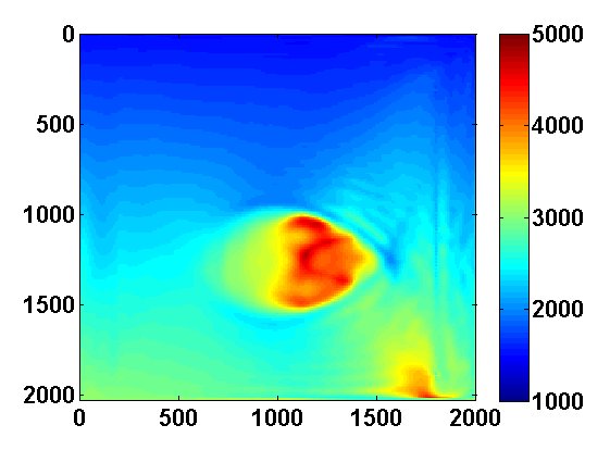
Since \(H^n\) is diagonal and positive, it is straightforward to add the constraint \(m \in [B_1 , B_2]\). In fact \[ \begin{equation} \label{bounds} \begin{aligned} \dm & = \arg \min_{\dm} \dm^T \nabla G(m^n) + \frac{1}{2}\dm^T H^n \dm + c_n \dm^T\dm \\ & \text{such that} \ m^n + \dm \in [B_1 , B_2] \end{aligned} \end{equation} \] has a closed form solution in this case. Even with these bound constraints, the model recovered using the penalty formulation can still contain artifacts and spurious oscillations, as shown in Figure 2. A simple and effective way to reduce oscillations in \(m\) via a convex constraint is to constrain its total variation (TV) to be less than some positive parameter \(\tau\). TV penalties are widely used in image processing to remove noise while preserving discontinuities (Rudin, Osher, & Fatemi, 1992). It is also a useful regularizer in a wide variety of other inverse problems, especially when solving for piecewise constant or piecewise smooth unknowns. For example, TV regularization has been successfully used for electrical inverse tomography (Chung, Chan, & Tai, 2005) and inverse wave propagation (Akcelik, Biros, & Ghattas, 2002). Although the problem is similar, the formulation in (Akcelik et al., 2002) is different that what we are considering here.

Total Variation Regularization

If we represent \(m\) as a \(N_1\) by \(N_2\) image, we can define \[ \begin{equation} \label{TVim} \begin{aligned} \|m\|_{TV} & = \frac{1}{h}\sum_{ij}\sqrt{(m_{i+1,j}-m_{i,j})^2 + (m_{i,j+1}-m_{i,j})^2} \\ & = \sum_{ij}\frac{1}{h}\left\| \bbm (m_{i,j+1}-m_{i,j})\\ (m_{i+1,j}-m_{i,j}) \ebm \right\| \ , \end{aligned} \end{equation} \] which is a sum of the \(l_2\) norms of the discrete gradient at each point in the discretized model. Assume Neumann boundary conditions so that these differences are zero at the boundary. We can represent \(\|m\|_{TV}\) more compactly by defining a difference operator \(D\) such that \(Dm\) is a concatenation of the discrete gradients and \((Dm)_n\) denotes the vector corresponding to the discrete gradient at the location indexed by \(n\), \(n = 1,...,N_1N_2\). Then we can define \[ \begin{equation} \label{TVvec} \|m\|_{TV} = \|Dm\|_{1,2} := \sum_{n=1}^N \|(Dm)_n\| \ . \end{equation} \] Returning to (\(\ref{SGD}\)), if we add the constraints \(m \in [B_1 , B_2]\) and \(\|m\|_{TV} \leq \tau\), then the overall iterations for solving \[ \begin{equation} \label{QP} \min_m G(m) \qquad \text{such that} \qquad m \in [B_1 , B_2] \text{ and } \|m\|_{TV} \leq \tau \end{equation} \] have the form \[ \begin{equation} \label{pTVb} \begin{aligned} \dm & = \arg \min_{\dm} \dm^T \nabla G(m^n) + \frac{1}{2}\dm^T H^n \dm + c_n \dm^T\dm \\ & \text{such that } m^n + \dm \in [B_1 , B_2] \text{ and } \|m^n + \dm\|_{TV} \leq \tau \\ m^{n+1} & = m^n + \dm \ . \end{aligned} \end{equation} \]

Solving the Convex Subproblems

An effective approach for solving the convex subproblems in (\(\ref{pTVb}\)) for \(\dm\) is to use a modification of the primal dual hybrid gradient (PDHG) method (Zhu & Chan, 2008) discussed in (Chambolle & Pock, 2011; Esser, Zhang, & Chan, 2010; He & Yuan, 2012; Zhang, Burger, & Osher, 2010) that finds a saddle point of \[ \begin{equation} \label{Lagrangian} \begin{aligned} \L(\dm,p) & = \dm^T \nabla G(m^n) + \frac{1}{2}\dm^T (H^n+2c_n\I) \dm \\ & + p^T D(m^n + \dm) - \tau \|p\|_{\infty,2} \end{aligned} \end{equation} \] for \(m^n + \dm \in [B_1 , B_2]\). Here, \(\|\cdot\|_{\infty,2}\) denotes the dual norm of \(\|\cdot\|_{1,2}\) and takes the max instead of the sum of the \(l_2\) norms. The modified PDHG method requires iterating \[ \begin{equation} \label{PDHGM} \begin{aligned} p^{k+1} & = \arg \min_p \tau \|p\|_{\infty,2} - p^T D(m^n + \dm^k) + \frac{1}{2 \delta}\|p - p^k\|^2 \\ \dm^{k+1} & = \arg \min_{\dm} \dm^T \nabla G(m^n) + \frac{1}{2}\dm^T (H^n+2c_n\I) \dm \\ & + \dm^T D^T(2p^{k+1}-p^k) + \frac{1}{2 \alpha}\|\dm - \dm^k\|^2 \\ & \text{such that } m^n + \dm \in [B_1 , B_2] \ . \end{aligned} \end{equation} \] These iterations can be written more explicitly as \[ \begin{equation} \label{PDHGexplicit} \begin{aligned} p^{k+1} & = p^k + \delta D(m^n + \dm^k) - \Pi_{\|\cdot\|_{1,2} \leq \tau \delta}(p^k + \delta D(m^n + \dm^k)) \\ \dm^{k+1} & = (H^n + \xi_n\I)^{-1} \max\left( (H^n + \xi_n\I)(B_1 - m^n), \right.\\ & \min\left( (H^n + \xi_n\I)(B_2 - m^n), \right.\\ & \left. \left. -\nabla G(m^n) + \frac{\dm^k}{\alpha} - D^T(2p^{k+1}-p^k) \right) \right) \ , \end{aligned} \end{equation} \] where \(\xi_n = 2c_n+\frac{1}{\alpha}\) and \(\Pi_{\|\cdot\|_{1,2} \leq \tau \delta}(z)\) denotes the orthogonal projection of \(z\) onto the ball of radius \(\tau \delta\) in the \(\|\cdot\|_{1,2}\) norm. Computing this projection is of equivalent difficulty as projecting onto a simplex, which can be done efficiently. The step size restriction required for convergence is \(\alpha \delta \leq \frac{1}{\|D^TD\|}\). If \(h\) is the mesh width, then it suffices to choose positive \(\alpha\) and \(\delta\) such that \(\alpha \delta \leq \frac{h^2}{8}\).

Numerical Experiments

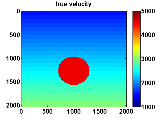
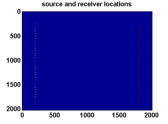
We consider a 2D synthetic experiment with a roughly \(200\) by \(200\) sized model and a mesh width \(h\) equal to \(10\) meters. The synthetic velocity model shown in Figure 1a has a constant high velocity region surrounded by a slower smooth background. We use an estimate of the smooth background as our initial guess \(m^0\). Similar to Example 1 in (T. van Leeuwen & Herrmann, 2013b), we put \(N_s = 34\) sources on the left and \(N_r = 81\) receivers on the right as shown in Figure 1b. The sources \(q_{sv}\) correspond to a Ricker wavelet with a peak frequency of \(30\)Hz.

Data is synthesized at \(18\) different frequencies ranging from \(3\) to \(20\) Hertz. We consider both noise free and slightly noisy data. In the noisy case, random Gaussian noise was added to the data \(d_v\) independently for each frequency index \(v\) and with standard deviations of \(\frac{.05 \|d_v\|}{\sqrt{N_s N_r}}\). This may not be a realistic noise model, but it can at least indicate that the method is robust to a small amount of noise in the data.

Three different choices for the regularization parameter \(\tau\) are considered: \(\tau_{\text{opt}}\), which is chosen to be the total variation of the true slowness squared, \(\tau_{\text{large}} = 1000\tau_{\text{opt}}\), which is large enough so that the total variation constraint has no effect, and \(\tau_{\text{small}} = .875\tau_{\text{opt}}\), slightly smaller than what would seem to be the optimal choice. Note that by using the Gauss Newton step from (\(\ref{bounds}\)) as an initial guess, the convex subproblem in (\(\ref{pTVb}\)) converges immediately in the \(\tau_{\text{large}}\) case. The parameter \(\lambda\) for the PDE penalty is fixed at 1 for all experiments.

We loop through the frequencies from low to high in overlapping batches of two, starting with the \(3\) and \(4\)Hz data, using the computed \(m\) as an initial guess for inverting the \(4\) and \(5\)Hz data and so on. For each frequency batch, we compute \(50\) outer iterations each time solving the convex subproblem to convergence, stopping when \(\max(\frac{\|p^{k+1}-p^k\|}{\|p^{k+1}\|},\frac{\|\dm^{k+1}-\dm^k\|}{\|\dm^{k+1}\|}) \leq 1\text{e}^{-5}\).

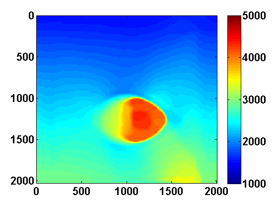
Results of the six experiments are shown in Figure 2. In both the noise free and noisy cases, including TV regularization reduced oscillations in the recovered model and led to better estimates of the high velocity region. Counterintuitively, the locations of the discontinuities were better estimated from noisy data than from noise free data. This likely happened because the noise caused there to be larger discontinuities at the receivers which then strengthened the effect of the TV regularization elsewhere. This is supported by the experiments with \(\tau_{\text{small}}\), which show that increasing the amount of TV regularization leads to better resolution of the large discontinuities but at the cost of losing contrast and staircasing the smooth background. There is also a risk of completely missing small discontinuities when \(\tau\) is chosen to be too small.

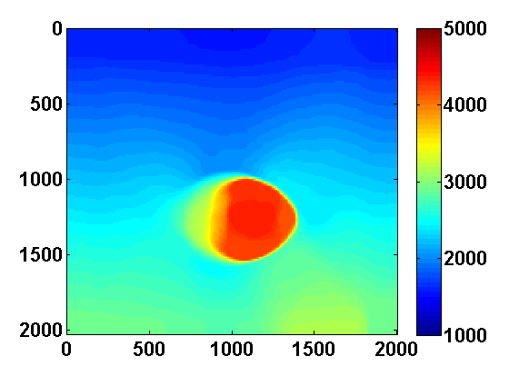
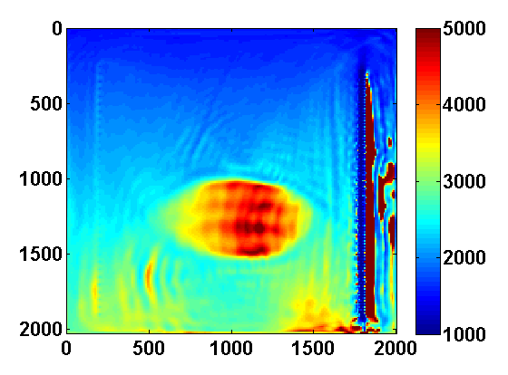
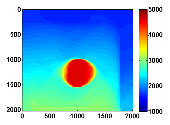
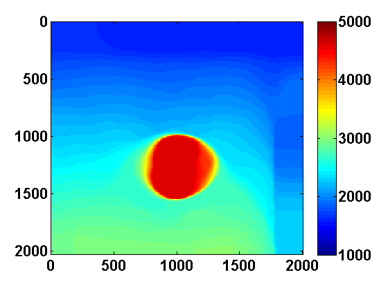
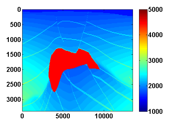
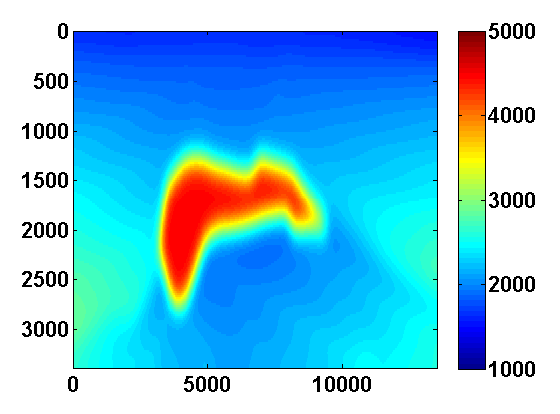
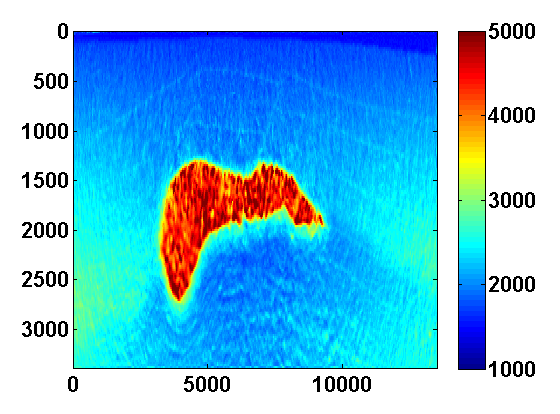
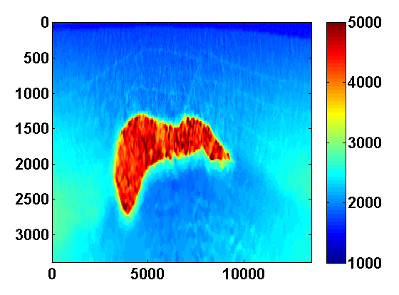
We also consider a synthetic experiment with simultaneous shots. The true velocity model is a \(170\) by \(676\) 2D slice from the SEG/EAGE salt model shown in Figure 3a. A total of \(116\) sources and \(676\) receivers were placed near the surface. The problem size is reduced by considering \(N_{ss} < N_s\) random mixtures of the sources \(q_{sv}\) defined by \[ \begin{equation} \label{simulshot} \bar{q}_{jv} = \sum_{s=1}^{N_s} w_{js}q_{sv} \qquad j = 1,...,N_{ss} \ , \end{equation} \] where the weights \(w_{js} \in \N(0,1)\) are drawn from a standard normal distribution. We modify the synthetic data according to \(\bar{d}_{jv} = P A_v^{-1}(m)\bar{q}_{jv}\) and use the same strategy to solve the smaller problem \[ \begin{equation} \label{altminss} \begin{aligned} \min_{m,u} & \sum_{jv} \frac{1}{2}\|P u_{jv} - \bar{d}_{jv}\|^2 + \frac{\lambda^2}{2}\|A_v(m)u_{jv} - \bar{q}_{jv}\|^2 \\ & \text{such that} \qquad m \in [B_1 , B_2] \text{ and } \|m\|_{TV} \leq \tau \ . \end{aligned} \end{equation} \] Starting with a good smooth initial model, results using two simultaneous shots with no added noise and for two values of \(\tau\) are shown in Figure 3. With only two simultaneous shots the number of PDE solves is resuced by almost a factor of \(60\). TV regularization helps remove some of the artifacts caused by using so few simultaneous shots and in this case mainly reduces noise under the salt.

Conclusions and Future Work

We presented a computationally feasible scaled gradient projection algorithm for minimizing the quadratic penalty formulation for full waveform inversion proposed in (T. van Leeuwen & Herrmann, 2013b) subject to additional convex constraints. We showed in particular how to solve the convex subproblems that arise when adding total variation and bound constraints on the model. Synthetic experiments suggest that when there is noisy or limited data TV regularization can improve the recovery by eliminating spurious artifacts and by more precisely identifying the locations of discontinuities.

In future work, we still need to find a practical way of selecting the regularization parameter \(\tau\). The fact that significant discontinuities can be resolved using small \(\tau\) suggests that a continuation strategy that gradually increases \(\tau\) could be effective. It will be interesting to investigate to what extent this strategy can avoid undesirable local minima. A possible numerical framework for this could be along the lines of the SPOR-SPG method in (Berg & Friedlander, 2011). We also intend to study more realistic numerical experiments.

Acknowledgements

Thanks to Bas Peters for insights about the formulation and implementation of the penalty method for full waveform inversion, and thanks also to Polina Zheglova for helpful discussions about the boundary conditions. This work was financially supported in part by the Natural Sciences and Engineering Research Council of Canada Discovery Grant (RGPIN 261641-06) and the Collaborative Research and Development Grant DNOISE II (CDRP J 375142-08). This research was carried out as part of the SINBAD II project with support from the following organizations: BG Group, BGP, BP, Chevron, ConocoPhillips, CGG, ION GXT, Petrobras, PGS, Statoil, Total SA, WesternGeco, Woodside.

References

Akcelik, V., Biros, G., & Ghattas, O. (2002). Parallel multiscale Gauss-Newton-Krylov methods for inverse wave propagation. Supercomputing, ACM/IEEE …, 00(c), 1–15. Retrieved from http://ieeexplore.ieee.org/xpls/abs\_all.jsp?arnumber=1592877
Aravkin, A. Y., & Leeuwen, T. van. (2012). Estimating nuisance parameters in inverse problems. Inverse Problems, 28(11), 115016. Retrieved from http://arxiv.org/abs/1206.6532
Berg, E. van den, & Friedlander, M. P. (2011). Sparse Optimization with Least-Squares Constraints. SIAM Journal on Optimization, 21(4), 1201–1229. doi:10.1137/100785028
Bertsekas, D. P. (1999). Nonlinear Programming (p. 780). Athena Scientific; 2nd edition. Retrieved from http://www.amazon.com/Nonlinear-Programming-Dimitri-P-Bertsekas/dp/1886529000/ref=sr\_1\_2?ie=UTF8\&qid=1395180760\&sr=8-2\&keywords=nonlinear+programming
Chambolle, A., & Pock, T. (2011). A first-order primal-dual algorithm for convex problems with applications to imaging. Journal of Mathematical Imaging and Vision. Retrieved from http://link.springer.com/article/10.1007/s10851-010-0251-1
Chung, E. T., Chan, T. F., & Tai, X.-C. (2005). Electrical impedance tomography using level set representation and total variational regularization. Journal of Computational Physics, 205(1), 357–372. doi:10.1016/j.jcp.2004.11.022
Esser, E., Lou, Y., & Xin, J. (2013). A Method for Finding Structured Sparse Solutions to Nonnegative Least Squares Problems with Applications. SIAM Journal on Imaging Sciences, 6(4), 2010–2046. doi:10.1137/13090540X
Esser, E., Zhang, X., & Chan, T. F. (2010). A General Framework for a Class of First Order Primal-Dual Algorithms for Convex Optimization in Imaging Science. SIAM Journal on Imaging Sciences, 3(4), 1015–1046. doi:10.1137/09076934X
He, B., & Yuan, X. (2012). Convergence analysis of primal-dual algorithms for a saddle-point problem: from contraction perspective. SIAM Journal on Imaging Sciences, 1–35. Retrieved from http://epubs.siam.org/doi/abs/10.1137/100814494
Herrmann, F. J., Hanlon, I., Kumar, R., Leeuwen, T. van, Li, X., Smithyman, B., … Takougang, E. T. (2013). Frugal full-waveform inversion: From theory to a practical algorithm. The Leading Edge, 32(9), 1082–1092. doi:10.1190/tle32091082.1
Leeuwen, T. van, & Herrmann, F. J. (2013a). A penalty method for PDE-constrained optimization.
Leeuwen, T. van, & Herrmann, F. J. (2013b). Mitigating local minima in full-waveform inversion by expanding the search space. Geophysical Journal International, 195(1), 661–667. Retrieved from http://gji.oxfordjournals.org/cgi/doi/10.1093/gji/ggt258
Rudin, L., Osher, S., & Fatemi, E. (1992). Nonlinear total variation based noise removal algorithms. Physica D: Nonlinear Phenomena, 60, 259–268. Retrieved from http://www.sciencedirect.com/science/article/pii/016727899290242F
Tarantola, A. (1984). Inversion of seismic reflection data in the acoustic approximation. Geophysics, 49(8), 1259–1266. Retrieved from http://link.springer.com/article/10.1007/s10107-012-0571-6 http://arxiv.org/abs/1110.0895 http://library.seg.org/doi/abs/10.1190/1.1441754
Virieux, J., & Operto, S. (2009). An overview of full-waveform inversion in exploration geophysics. Geophysics, 74(6), WCC1–WCC26. doi:10.1190/1.3238367
Zhang, X., Burger, M., & Osher, S. (2010). A Unified Primal-Dual Algorithm Framework Based on Bregman Iteration. Journal of Scientific Computing, 46(1), 20–46. doi:10.1007/s10915-010-9408-8
Zhu, M., & Chan, T. (2008). An Efficient Primal-Dual Hybrid Gradient Algorithm For Total Variation Image Restoration. UCLA CAM Report [08-34], (1), 1–29.