Learned multiphysics inversion with differentiable programming and machine learning

![]()

Summary
We present the Seismic Laboratory for Imaging and Modeling/Monitoring (SLIM) open-source software framework for computational geophysics and, more generally, inverse problems involving the wave-equation (e.g., seismic and medical ultrasound), regularization with learned priors, and learned neural surrogates for multiphase flow simulations. By integrating multiple layers of abstraction, our software is designed to be both readable and scalable. This allows researchers to easily formulate their problems in an abstract fashion while exploiting the latest developments in high-performance computing. We illustrate and demonstrate our design principles and their benefits by means of building a scalable prototype for permeability inversion from time-lapse crosswell seismic data, which aside from coupling of wave physics and multiphase flow, involves machine learning.
Motivation
Thanks to major advancements in high-performance computing (HPC) techniques, computational (exploration) geophysics has made giant leaps over the past decades. These developments have, for instance, led to the adoption of wave-equation-based inversion technologies such as full-waveform inversion (FWI) and reverse-time migration (RTM) that, thanks to their adherence to wave physics, have resulted in superior imaging in complex geologies. While these techniques certainly rank amongst the most sophisticated imaging technologies, their implementation relies with few exceptions—most notably iWave++ (Sun and Symes 2010), Julia Devito Inversion framework (JUDI.jl of the Seismic Laboratory for Imaging and Modeling (SLIM), P. A. Witte, Louboutin, Kukreja, et al. (2019); Mathias Louboutin et al. (2023)), and Chevron’s COFII (Washbourne et al. 2021)—on monolithic low-level (C/Fortran) implementations. As a consequence, due to their lack of abstraction and modern programming constructs, these low-level implementations are difficult and very costly to maintain, especially when performance considerations prevail over best software practices. While these implementation design choices lead to performant code for specific problems, such as FWI, they often hinder the implementation of new algorithms, e.g., based on different objective functions or constraints, as well as coupling existing code bases with external software libraries. For instance, combining wave-equation-based inversion with machine learning frameworks or coupling wave-physics with multiphase fluid-flow solvers are considered challenging and costly. Thus, our industry runs the risk of losing its ability to innovate, a situation that is exacerbated by the challenges we face as a result of the energy transition.
Design principles
To address these important shortcomings of current software implementations that impede progress, we have embarked on the development of a performant software framework. For instance, our wave propagators, implemented in Devito (M. Louboutin et al. 2019; Luporini et al. 2020), are used in production by contractors and Oil & Gas majors while enabling rapid, low-cost, scalable, and interoperable algorithm development for multiphysics and machine learning problems that runs on a variety of different chipsets (e.g., ARM, Intel, POWER) and graphics accelerators (e.g., NVIDIA). To achieve this, we adopt contemporary software design practices that include high-level abstractions, software design principles, and the utilization of modern programming languages, such as Python (Rossum and Drake 2009) and Julia (Bezanson et al. 2017). We also make extensive use of abstractions provided by domain-specific languages (DSLs), such as the Rice Vector Library (RVL, Padula, Scott, and Symes 2009) and the Unified Form Language (UFL, Rathgeber et al. 2016; Alnaes et al. 2015), and adopt reproducible research practices introduced by the trailblazing open-source initiative Madagascar (Fomel et al. 2013), which successfully made use of version control and an abstraction based on the software construction tool SCons.
In an effort to meet the challenges of modern software design in a performance-critical environment, we adhere to three key principles—in addition to the fundamental principle of separation of concerns. First, we adopt mathematical language to inform our abstractions. Mathematics is concise, unambiguous, well understood, and leads to natural abstractions for the
- wave physics, through partial differential equations as put to practice by Devito, which relies on Symbolic Python (SymPy) (Meurer et al. 2017) to define partial differential equations. Given the symbolic expressions, Devito automatically generates highly-optimized, possibly domain-decomposed, parallel C code that targets the available hardware with near-optimal performance for 3D acoustic, tilted-transverse-isotropic, or elastic wave-equations;
- linear algebra, through matrix-free linear operators, as in JUDI.jl (P. A. Witte, Louboutin, Kukreja, et al. 2019; Mathias Louboutin et al. 2023)—a high-level linear algebra DSL for wave-equation-based modeling and inversion. These ideas date back to SPOT (Berg and Friedlander 2009) with more recent implementations JOLI.jl (Modzelewski et al. 2023) in Julia and PyLops in Python (Ravasi and Vasconcelos 2020).
- optimization, through definition of objective functions, also known as loss functions, that need to be minimized—via SlimOptim.jl (Mathias Louboutin, Yin, and Herrmann 2022b)—subject to mathematical constraints, which can be imposed through SetIntersectionProjection.jl (Peters and Herrmann 2019; Peters, Louboutin, and Modzelewski 2022).
Second, we exploit hierarchy within wave-equation-based inversion problems that naturally leads to a separation of concerns. At the highest level, we deal with linear operators, specifically matrix-free Jacobians of wave-based inversion, with JUDI.jl and parallel file input/output with SegyIO.jl (Lensink et al. 2023) on premise, or in the Cloud (Azure) via JUDI4Cloud.jl (Mathias Louboutin, Yin, and Herrmann 2022a). At the intermediate and lower level, we make extensive use of Devito (M. Louboutin et al. 2019; Luporini et al. 2020)—a just-in-time compiler for stencil-based time-domain finite-difference calculations, the development of which SLIM has been involved in over the years.
Third, we build on the principles of differentiable programming as advocated by Mike Innes et al. (2019) and intrusive automatic differentiation introduced by D. Li et al. (2020) to integrate wave-physics with machine learning frameworks and multiphase flow. Specifically, we employ automatic differentiation (AD) through the use of the chain rule, including abstractions that allow the user to add derivative rules, as in ChainRules.jl (White et al. 2022, 2023).
During the Inaugural Full-Waveform Inversion Workshop in 2015, we at SLIM started to articulate these design principles (Lin and Herrmann 2015), which over the years cumulated in scalable parallel software frameworks for time-harmonic FWI (Silva and Herrmann 2019), for time-domain RTM and FWI (P. A. Witte, Louboutin, Kukreja, et al. 2019; Mathias Louboutin et al. 2023), and for abstracted FWI (Mathias Louboutin et al. 2022) allowing for connections with machine learning. Aside from developing software for wave-equation-based inversion, our group has more recently also been involved in the development of scalable machine learning solutions, including the Julia package InvertibleNetworks.jl (P. Witte et al. 2023, 2023), which implements memory-efficient invertible deep neural networks such as (conditional) normalizing flows (NFs, Rezende and Mohamed 2015), and scalable distributed Fourier neural operators (FNOs, Z. Li et al. 2020) in the dfno package (Grady et al. 2022; Grady, Infinoid, and Louboutin 2022). All of these will be described in more detail below.
To illustrate how these design principles can lead to solutions of complex learned coupled inversions, we consider in the ensuing sections end-to-end inversion of time-lapse seismic data for the spatial permeability distribution (D. Li et al. 2020). As can be seen from Figure 1, this inversion problem is rather complex and whose solution arguably benefits from our three design principles listed above. In this formulation, the latent representation for the permeability is taken via a series of nonlinear operations all the way to the time-lapse seismic data. In the remainder of this exposition, we will detail how the different components in this learned inversion problem are implemented so that the coupled inversion can be carried out. The results presented are preliminary representing a snapshot on how research is conducted according to the design principles.

Learned time-lapse end-to-end permeability inversion
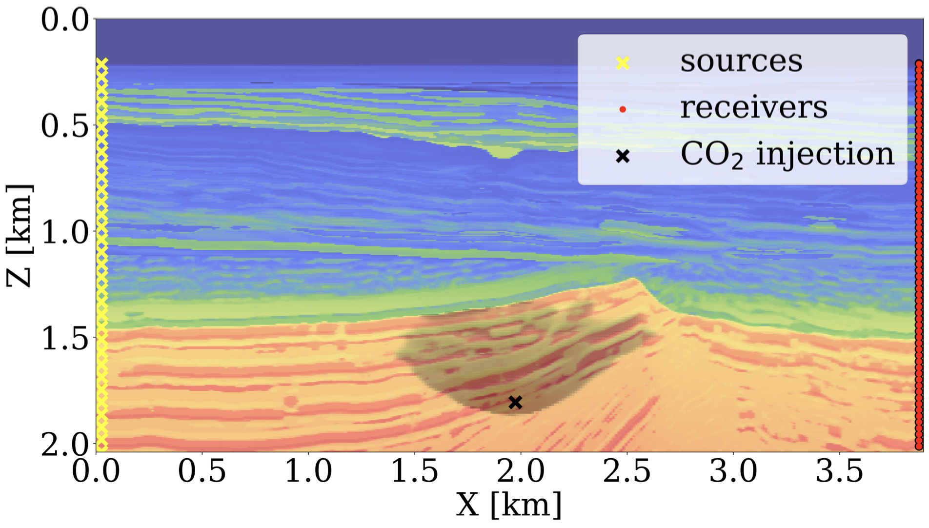
Combating climate change and dealing with the energy transition call for solutions to problems of increasing complexity. Building seismic monitoring systems for geological CO2 and/or H2 storage falls in this category. To demonstrate how math-inspired abstractions can help, we consider inversion of permeability from crosswell time-lapse data (see Figure 2 for experimental setup) involving (i) coupling of wave physics with two-phase (brine/CO2) flow using Jutul.jl (Møyner et al. 2023), state-of-the-art reservoir modeling software in Julia; (ii) learned regularization with NFs with InvertibleNetworks.jl; (iii) learned surrogates for the fluid-flow simulations with FNOs. This type of inversion problem is especially challenging because it involves different types of physics to estimate the past, current, and future saturation and pressure distributions of CO2 plumes from crosswell data in saline aquifers. In the subsequent sections, we demonstrate how we invert time-lapse data using the separate software packages listed in Figure 1.
Wave-equation-based inversion
Thanks to its unmatched ability to resolve CO2 plumes, active-source time-lapse seismic is arguably the preferred imaging modality when monitoring geological storage (Ringrose 2020). In its simplest form for a single time-lapse vintage, FWI involves minimizing the \(\ell_2\)-norm misfit/loss function between observed and synthetic data—i.e., we have
\[ \underset{\mathbf{m}}{\operatorname{minimize}} \quad \frac{1}{2}\|\mathbf{F}(\mathbf{m})\mathbf{q} - \mathbf{d} \|^2_2 \quad \text{where} \quad \mathbf{F}(\mathbf{m}) = \mathbf{P}_r {\mathbf{A}(\mathbf{m})}^{-1}\mathbf{P}_s^{\top}. \tag{1}\]
In this formulation, the symbol \(\mathbf{F}(\mathbf{m})\) represents the forward modeling operator (wave physics), parameterized by the squared slowness, \(\mathbf{m}\). This forward operator acting on the sources consists of the composition of source injection operator, \(\mathbf{P}^\top_s\) with \(^\top\) denoting the transpose operator, solution of the discretized wave equation via \({\mathbf{A}(\mathbf{m})}^{-1}\), and restriction to the receivers via the linear operator \(\mathbf{P}_r\). The vector \(\mathbf{q}\) represents the seismic sources and the vector \(\mathbf{d}\) contains single-vintage seismic data, collected at the receiver locations. Thanks to our adherence to the math, the corresponding Julia code to invert for the unknown squared slowness \(\mathbf{m}\) with JUDI.jl reads
# Forward modeling to generate seismic data.
Pr = judiProjection(recGeometry)  # setup receiver
Ps = judiProjection(srcGeometry)  # setup sources
Ainv = judiModeling(model)        # setup wave-equation solver
F = Pr * Ainv * Ps'               # forward modeling operator
d = F(m_true) * q                 # generate observed data
# Gradient descent to invert for the unknown squared slowness.
for it = 1:maxiter
    d0 = F(m) * q                 # generate synthetic data
    J = judiJacobian(F(m), q)     # setup the Jacobian operator of F
    g = J' * (d0 - d)             # gradient w.r.t. squared slowness
    m = m - t * g                 # gradient descent with steplength t
end
To obtain this concise and abstract formulation for FWI, we utilized hierarchical abstractions for propagators in Devito and linear algebra tools in JUDI.jl, including matrix-free implementations for F and its Jacobian J. While the above stand-alone implementation allows for (sparsity-promoting) seismic (P. A. Witte, Louboutin, Luporini, et al. 2019; Herrmann, Siahkoohi, and Rizzuti 2019; Yang et al. 2020; Rizzuti et al. 2020, 2021; Siahkoohi, Rizzuti, and Herrmann 2020a, 2020b, 2020c; Yin, Louboutin, and Herrmann 2021; Yin et al. 2023) and medical (Yin et al. 2020; Orozco et al. 2021, 2023; Orozco, Louboutin, et al. 2023) inversions, it relies on hand-derived implementations for the adjoint of the Jacobian J' and for the derivative of the loss function. Although this approach is viable, relying solely on hand-derived derivatives can become cumbersome when we want to utilize machine learning models or when we need to couple the wave equation to the multiphase flow equation.
To allow for this situation, we make use of Julia’s differentiable programming ecosystem that includes tools to use AD and to add differentiation rules via ChainRules.jl. Using this tool, the AD system can be taught how to differentiate JUDI.jl via the following differentiation rule for the forward propagator
# Custom AD rule for wave modeling operator.
function rrule(::typeof(*), F::judiModeling, q)
    y = F * q                     # forward modeling
    # The pullback function for gradient calculations.
    pullback(dy) = NoTangent(), judiJacobian(F, q)' * dy, F' * dy
    return y, pullback
end
In this rule, the pullback function takes as input the data residual, dy, and outputs the gradient with respect to the operator * (no gradient), the model parameters, and the source distribution. With this differentiation rule, the above gradient descent algorithm can be implemented as follows:
# Define the loss function.
loss(m) = .5f0 * norm(F(m) * q - d)^2f0
# Gradient descent to invert for the squared slowness.
for it = 1:maxiter
    g = gradient(loss, m)[1]      # gradient computation via AD
    m = m - t * g                 # gradient descent with steplength t
end
Compared to the original implementation, this code only needs F(m) and the function loss(m). With the help of the above rrule, Julia’s AD system1 is capable of computing the gradients (line 5). Aside from remaining performant, i.e., we still make use of the adjoint-state method to compute the gradients, the advantage of this approach is that it allows for much more flexibility, e.g., in situations where the squared slowness is parameterized in terms of a pretrained neural network or in terms of the output of multiphase flow simulations. In the next section, we show how trained NFs can serve as priors to improve the quality of FWI.
Deep priors and normalizing flows
NFs are generative models that take advantage of invertible deep neural network architectures to learn complex distributions from training examples (Dinh, Sohl-Dickstein, and Bengio 2016). For example, in seismic inversion applications, we are interested in approximating the distribution of Earth models to use as priors in downstream tasks. NFs learn to map samples from the target distribution (i.e., Earth models) to zero-mean unit standard deviation Gaussian noise using a sequence of trainable nonlinear invertible layers. Once trained, one can resample new Gaussian noise and pass it through the inverse sequence of layers to obtain new generative samples from the target distribution. NFs are an attractive choice for generative models in seismic applications (Zhang and Curtis 2020, 2021; Zhao, Curtis, and Zhang 2021; Siahkoohi and Herrmann 2021; Siahkoohi et al. 2021, 2023; Siahkoohi, Rizzuti, and Herrmann 2022) because they provide fast sampling and allow for memory-efficient training due to their intrinsic invertibility, which eliminates the need to store intermediate activations during backpropagation. Memory efficiency is particularly important for seismic applications due to the 3D volumetric nature of the seismic models. Thus, our methods need to scale well in this regime.
To illustrate the practical use of NFs as priors in seismic inverse problems, we trained an NF on slices from the Compass model (Jones et al. 2012). In Figure 4, we compare generative samples from the NF with the slices used to train the model shown in Figure 3. Although there are still irregularities, the model has learned important qualitative aspects of the model that will be useful in inverse problems. To demonstrate this usefulness, we test our prior on an FWI inverse problem. Because our NF prior is trained independently, it is flexible and can easily be plugged into different inverse problems.


Our FWI experiment includes: ocean bottom nodes, Ricker wavelet with no energy below 4Hz, additive colored Gaussian noise that has the same bandwidth as the noise-free data. For FWI with our learned prior, we minimize
\[ \underset{\mathbf{z}}{\operatorname{minimize}} \quad \frac{1}{2}\|\mathbf{F}(\mathcal{G}_{\theta^\ast}(\mathbf{z}))\mathbf{q} - \mathbf{d}\|^2_2 + \frac{\lambda}{2}\|\mathbf{z}\|^2_2, \tag{2}\]
where \(\mathcal{G}_{\theta^\ast}\) is a pretrained NF with weights \(\theta^\ast\). After training, the inverse of the NF maps realistic Compass-like Earth samples to white noise—i.e., \(\mathcal{G}^{-1}_{\theta^\ast}(\mathbf{m}) = \mathbf{z} \sim \mathcal{N}(0, I)\). Since the NFs are designed to be invertible, the action of the pretrained NF, \({\mathcal{G}_{\theta^\ast}}\), on Gaussian noise \(\mathbf{z}\) produces realistic samples of Earth models (see Figure 4). We use this capability in the above equation where the unknown model parameters in \(\mathbf{m}\) are reparameterized by \(\mathcal{G}_{\theta^\ast}(\mathbf{z})\). The regularization term, \(\frac{\lambda}{2}\|\mathbf{z}\|^2_2\), penalizes the latent variable \(\mathbf{z}\) with large \(\ell_2\) norm, where \(\lambda\) balances the misfit and regularization terms. Consequently, this learned regularizer encourages FWI results that are more likely to be realistic Earth models (Asim et al. 2020). However, notice that the optimization routine now requires differentiation through both the physical operator (wave physics, \(\mathbf{F}\)) and the pretrained NF (\(\mathcal{G}_{\theta^\ast}\)), and only a true invertible implementation like ours, with minimal memory imprint for both training and inference, can provide scalability.
Thanks to the JUDI.jl’s rrule for F and InvertibleNetworks.jl’s rrule for G, integration of machine learning with FWI becomes straightforward involving replacement of m by G(z) on line 6. Minimizing the objective function in Equation 2 now translates to
# Load the pretrained NF and weights.
G = NetworkGlow(nc, nc_hidden, depth, nscales)
set_params!(G, θ)
# Set up the ADAM optimizer.
opt = ADAM()
# Define the reparameterized loss function including penalty term.
loss(z) = .5f0 * norm(F(G(z)) * q - d)^2f0 + .5f0 * λ * norm(z)^2f0
# ADAM iterations.
for it = 1:maxiter
g = gradient(loss, z)[1] # gradient computation with AD
update!(opt, z, g) # update z with ADAM
end
# Convert latent variable to squared slowness.
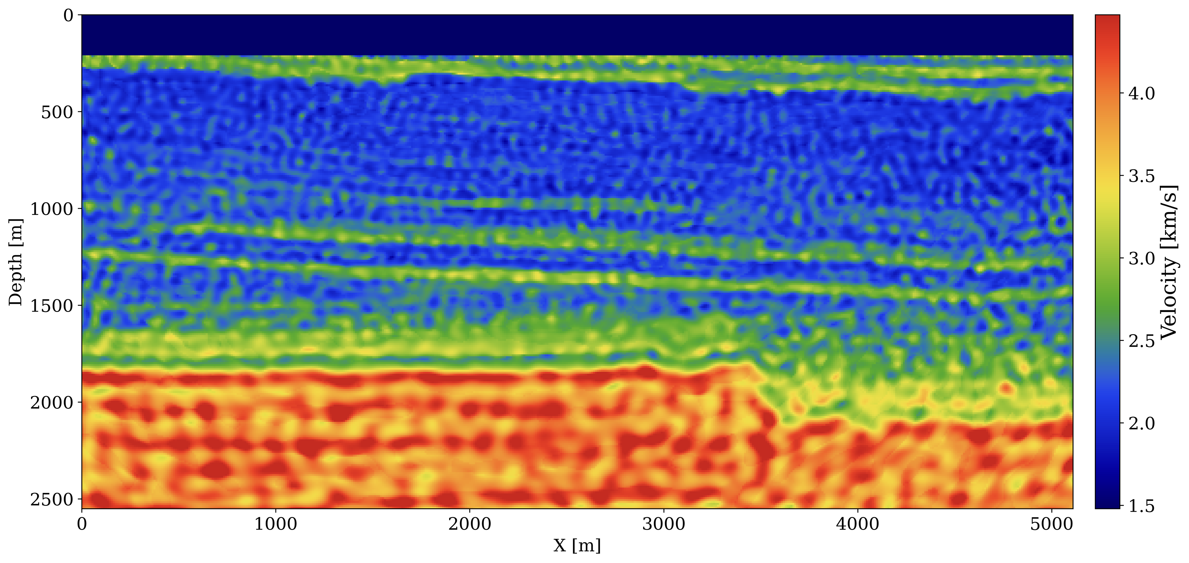
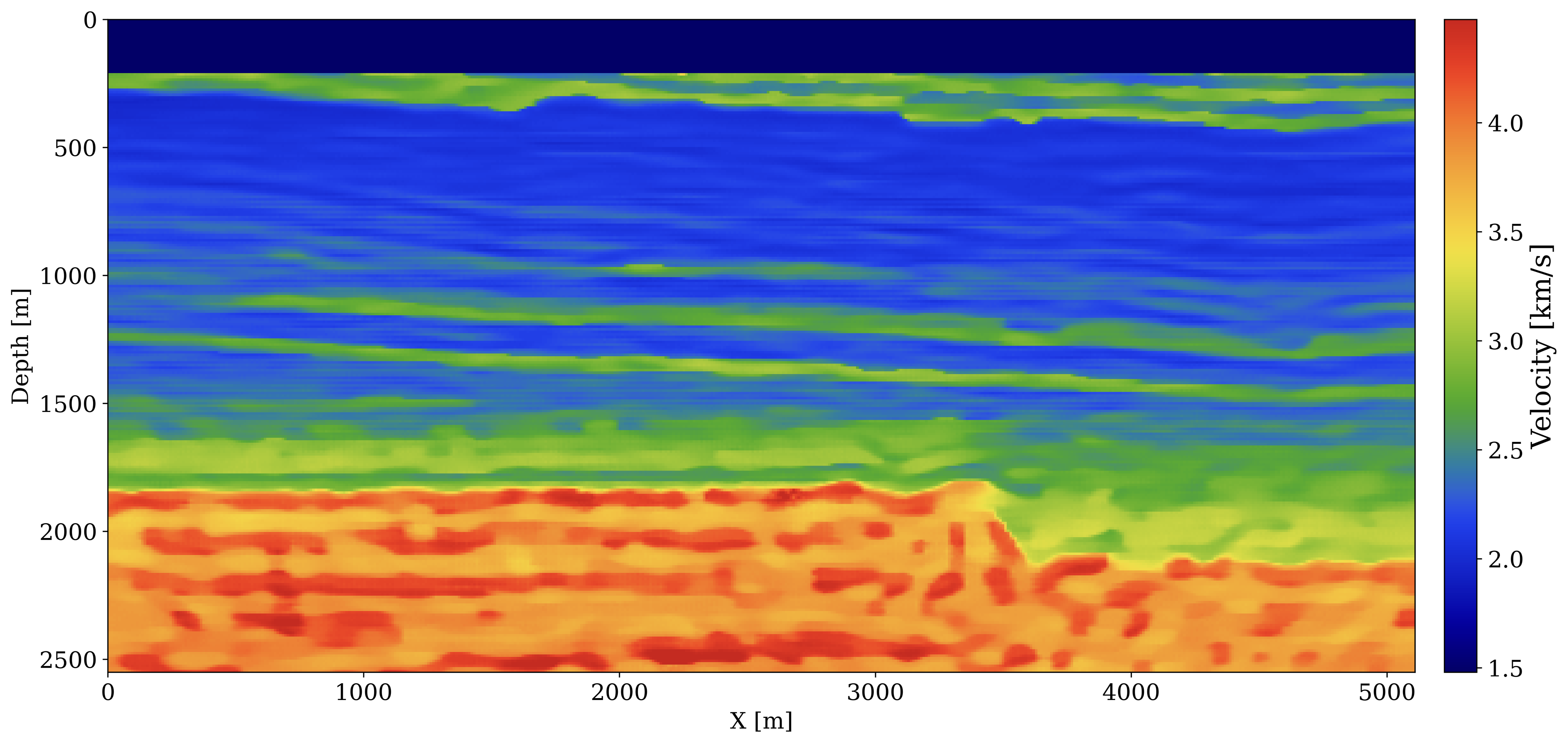
m = G(z)In Figure 5, we compare the results of FWI with our learned prior against unregularized FWI. Since our prior regularizes the solution towards realistic models, we obtain a velocity estimate that is closer to the ground truth.

Through this simple example, we demonstrated the ability to easily integrate our state-of-the-art wave-equation propagators with the Julia’s differentiable programming system. By applying these design principles to other components of the end-to-end inversion, we design a seismic monitoring framework for real-world applications in subsurface reservoirs.
Fluid-flow simulation and permeability inversion
As stated earlier, our goal is to estimate the permeability from time-lapse crosswell monitoring data collected at a CO2 injection site (cf. Figure 2). Compared to conventional seismic imaging, time-lapse monitoring of geological storage differs because it aims to image time-lapse changes in the CO2 plume while obtaining estimates for the reservoir’s fluid-flow properties. This involves coupling wave modeling operators to fluid-flow physics to track the CO2 plumes underground. The fluid-flow physics models the slow process of CO2 partly replacing brine in the pore space of the reservoir, which involves solving the multiphase flow equations. For this purpose, we need access to reservoir simulation software capable of modeling two-phase (brine/CO2) flow. While a number of proprietary and open-source reservoir simulators exist, including MRST (Lie and Møyner 2021), GEOSX (Settgast et al. 2022) and Open Porous Media (OPM) (Rasmussen et al. 2021), few support differentiation of the simulator’s output (CO2 saturation) with respect to its input (the spatial permeability distribution \(\mathbf{K}\) in Figure 1). We use the recently developed external Julia package JutulDarcy.jl that supports Darcy flow and serves as a front-end to Jutul.jl (Møyner et al. 2023), which provides accurate Jacobians with respect to \(\mathbf{K}\). Jutul.jl is an implicit solver for finite-volume discretizations that internally uses AD to calculate the Jacobian. It has a performance and feature set comparable to commercial multiphase flow simulators and accounts for realistic effects (e.g., dissolution, inter-phase mass exchange, compressibility, capillary effects) and residual trapping mechanisms. It also provides accurate sensitivities through an adjoint formulation of the subsurface multiphase flow equations. To integrate the Jacobian of this software package into Julia’s differentiable programming system, we wrote the light “wrapper package” JutulDarcyRules.jl (Yin and Louboutin 2023) that adds an rrule for the nonlinear operator \(\mathcal{S}(\mathbf{K})\), which maps the permeability distribution, \(\mathbf{K}\), to the spatially-varying CO2 concentration snapshots, \(\mathbf{c}=\{\mathbf{c}^{i}\}_{i=1}^{n_v}\), over \(n_v\) monitoring time-steps (cf. Figure 1). Addition of this rrule allows these packages to interoperate with other packages in Julia’s AD ecosystem. Below, we show a basic example where ADAM algorithm is used to invert for subsurface permeability given the full history of CO2 concentration snapshots:
# Generate CO2 concentration.
c = S(K_true)
# Set up ADAM optimizer.
opt = ADAM()
# Define the loss function.
loss(K) = .5f0 * norm(S(K) - c)^2f0
# ADAM iterations.
for it = 1:maxiter
    g = gradient(loss, K)[1]      # gradient computed with AD
    update!(opt, K, g)            # update K with ADAM
end
During each iteration of the loop above, Julia’s machine learning package Flux.jl (Michael Innes et al. 2018; Mike Innes 2018) uses the custom gradient defined by the aforementioned rrule, calling the high-performance adjoint code from JutulDarcy.jl. Our adaptable software framework also facilitates effortless substitution of deep learning models in lieu of the numerical fluid-flow simulator. In the next section, we introduce distributed Fourier neural operators (dfno) and discuss how this neural surrogate contributes to our inversion framework.
Fourier neural operator surrogates
While the integration of multiphase flow modeling into Julia differentiable programming ecosystem opens the way to carry out end-to-end inversions (as explained below), fluid-flow simulations are computationally expensive—a notion compounded by the fact that these simulations have to be done many times during inversion. For this reason, we switch to a data-driven approach where a neural operator is first trained on simulation examples, pairs \(\{\mathbf{K},\, \mathcal{S}(\mathbf{K})\}\), to learn the mapping from permeability models, \(\mathbf{K}\), to the corresponding CO2 snapshots, \(\mathbf{c} := \mathcal{S}(\mathbf{K})\). After incurring initial offline training costs, this neural surrogate provides a fast alternative to numerical solvers with acceptable accuracy. Fourier neural operators (FNOs, Z. Li et al. 2020), a recently introduced neural network architecture, have been used successfully to simulate two-phase flow during geological CO2 storage projects (Wen et al. 2022). Independently, Yin et al. (2022) used a trained FNO to replace the fluid-flow simulations as part of end-to-end inversion and showed that AD of Julia’s machine learning package can be used to compute gradients with respect to the permeability using Flux.jl’s reverse-mode AD system Zygote.jl (Michael Innes 2018). After training, the above permeability inversion from concentration snapshots, \(\mathbf{c}\), is carried out by simply replacing \(\mathcal{S}\) by \(\mathcal{S}_{\mathbf{w}^\ast}\) with \(\mathbf{w}^\ast\) being the weights of the pretrained FNO. Thanks to the AD system, the gradient with respect to \(\mathbf{K}\) is computed automatically. Thus, after loading the trained FNO and redefining the operator S, the above code remains exactly the same. For implementation details on the FNO and its training, we refer to Yin et al. (2022) and Grady et al. (2022).
Putting it all together
As a final step in our end-to-end permeability inversion, we introduce a nonlinear rock physics model, denoted by \(\mathcal{R}\). Based on the patchy saturation model (Avseth, Mukerji, and Mavko 2010), this model nonlinearly maps the time-lapse CO2 saturations to decreases in the seismic properties (compressional wavespeeds, \(\mathbf{v}=\{\mathbf{v}^{i}\}_{i=1}^{n_v}\)) within the reservoir with the Julia code
# Patchy saturation function.
# Input: CO2 saturation, velocity, density, porosity.
# Optional: bulk modulus of mineral, brine, CO2; density of CO2, brine.
# Output: velocity, density.
function Patchy(sw, vp, rho, phi;
    bulk_min=36.6f9, bulk_fl1=2.735f9, bulk_fl2=0.125f9,
    ρw=7f2, ρo=1f3) where T
    # Relate vp to vs, set modulus properties.
    vs = vp ./ sqrt(3f0)
    bulk_sat1 = rho .* (vp.^2f0 .- 4f0/3f0 .* vs.^2f0)
    shear_sat1 = rho .* (vs.^2f0)
    # Calculate bulk modulus if filled with 100% CO2.
    patch_temp = bulk_sat1 ./ (bulk_min .- bulk_sat1)
        .- bulk_fl1 ./ phi ./ (bulk_min .- bulk_fl1)
        .+ bulk_fl2 ./ phi ./ (bulk_min .- bulk_fl2)
    bulk_sat2 = bulk_min ./ (1f0 ./ patch_temp .+ 1f0)
    # Calculate new bulk modulus as weighted harmonic average.
    bulk_new = 1f0 / ((1f0 .- sw) ./ (bulk_sat1 .+ 4f0/3f0 * shear_sat1)
    + sw ./ (bulk_sat2 + 4f0/3f0 * shear_sat1)) - 4f0/3f0 * shear_sat1
    # Calculate new density and velocity.
    rho_new = rho + phi .* sw * (ρw - ρo)
    vp_new = sqrt.((bulk_new .+ 4f0/3f0 * shear_sat1) ./ rho_new)
    return vp_new, rho_new
end
We map the changes in the wavespeeds to time-lapse seismic data, \(\mathbf{d}=\{\mathbf{d}^{i}\}_{i=1}^{n_v}\), via the blockdiagonal seismic modeling2 operator \(\mathcal{F}(\mathbf{v})=\operatorname{diag}\left(\left\{\mathbf{F}^{i}(\mathbf{v}^{i})\mathbf{q}^{i}\right\}_{i=1}^{n_v}\right)\). In this formulation, the single vintage forward operators \(\mathbf{F}^{i}\) and corresponding sources, \(\mathbf{q}^{i}\), are allowed to vary between vintages.
With the fluid-flow (surrogate) solver, \(\mathcal{S}\), the rock physics module, \(\mathcal{R}\), and wave physics module, \(\mathcal{F}\), in place, along with regularization via reparametrization using \(\mathcal{G}_{\theta^\ast}\), we are now in a position to formulate the desired end-to-end inversion problem as
\[ \underset{\mathbf{z}}{\operatorname{minimize}}\quad \frac{1}{2}\|\mathcal{F}\circ\mathcal{R}\circ\mathcal{S}\left(\mathcal{G}_{\theta^\ast}(\mathbf{z})\right)- \mathbf{d}\|^2_2 + \frac{\lambda}{2}\|\mathbf{z}\|^2_2, \tag{3}\]
where the inverted permeability can be calculated by \(\mathbf{K}^\ast=\mathcal{G}_{\theta^\ast}(\mathbf{z}^\ast)\) with \(\mathbf{z}^\ast\) the latent space minimizer of Equation 3. As illustrated in Figure 1, we obtain the nonlinear end-to-end map by composing the fluid-flow, rock, and wave physics, according to \(\mathcal{F}\circ\mathcal{R}\circ\mathcal{S}\). The corresponding Julia code reads
# Set up ADAM optimizer.
opt = ADAM()
# Define the reparameterized loss function including penalty term.
loss(z) = .5f0 * norm(F ∘ R ∘ S(G(z)) - d)^2f0 + .5f0 * λ * norm(z)^2f0
# ADAM iterations.
for it = 1:maxiter
    g = gradient(loss, z)[1]      # gradient computed by AD
    update!(opt, z, g)            # update z by ADAM
end
# Convert latent variable to permeability.
K = G(z)
This end-to-end inversion procedure, which utilizes a learned deep prior and a pretrained FNO surrogate, was successfully employed by Yin et al. (2022) on a simple stylistic blocky high-low permeability model. The procedure involves using AD, with rrule for the wave and fluid physics, in combination with innate AD capabilities to compute the gradient of the objective in Equation 3, which incorporates fluid-flow, rock, and wave physics. Below, we share early results from applying the proposed end-to-end inversion in a more realistic setting derived from real data (cf. Figure 2).
Preliminary inversion results
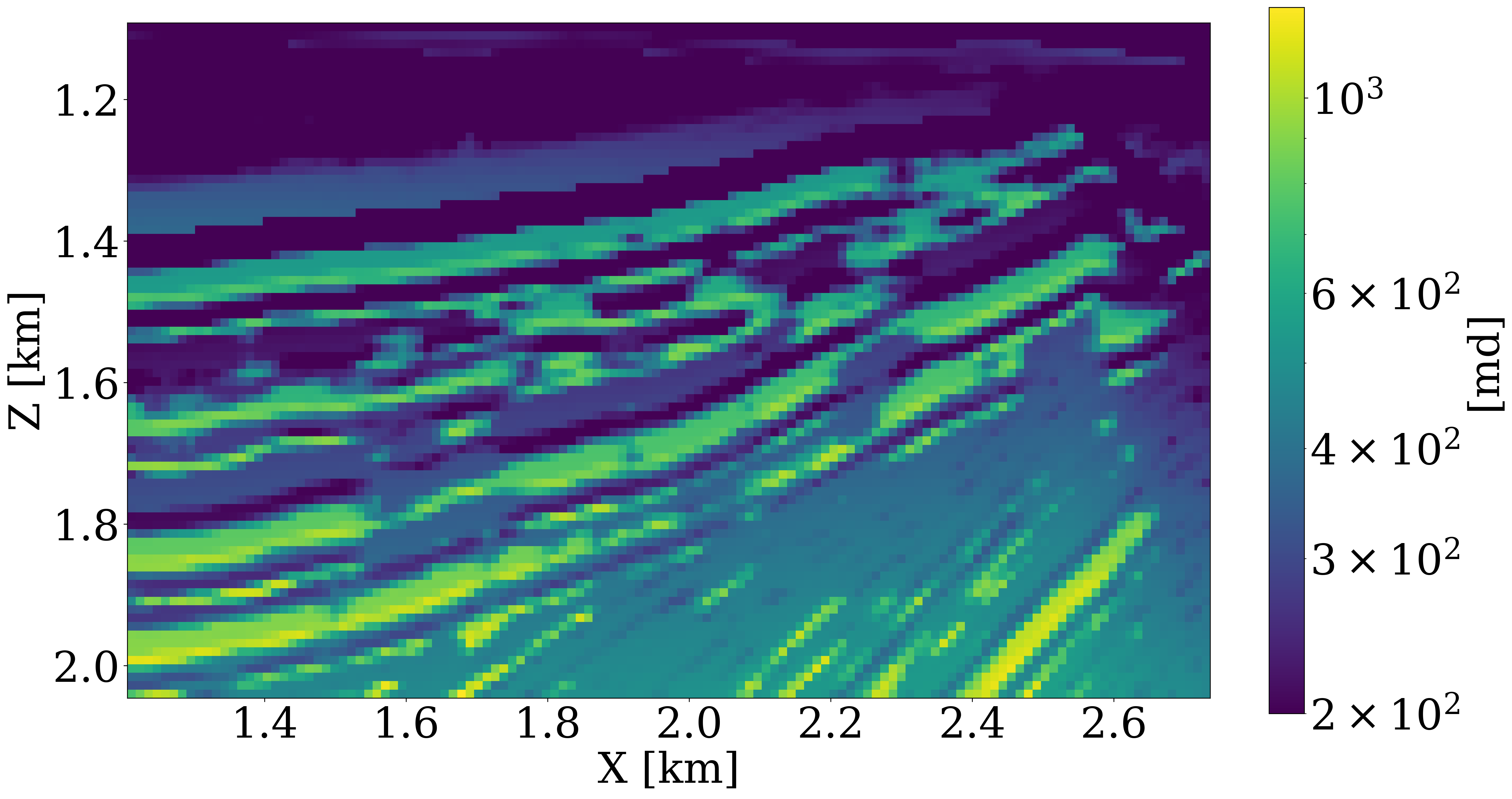
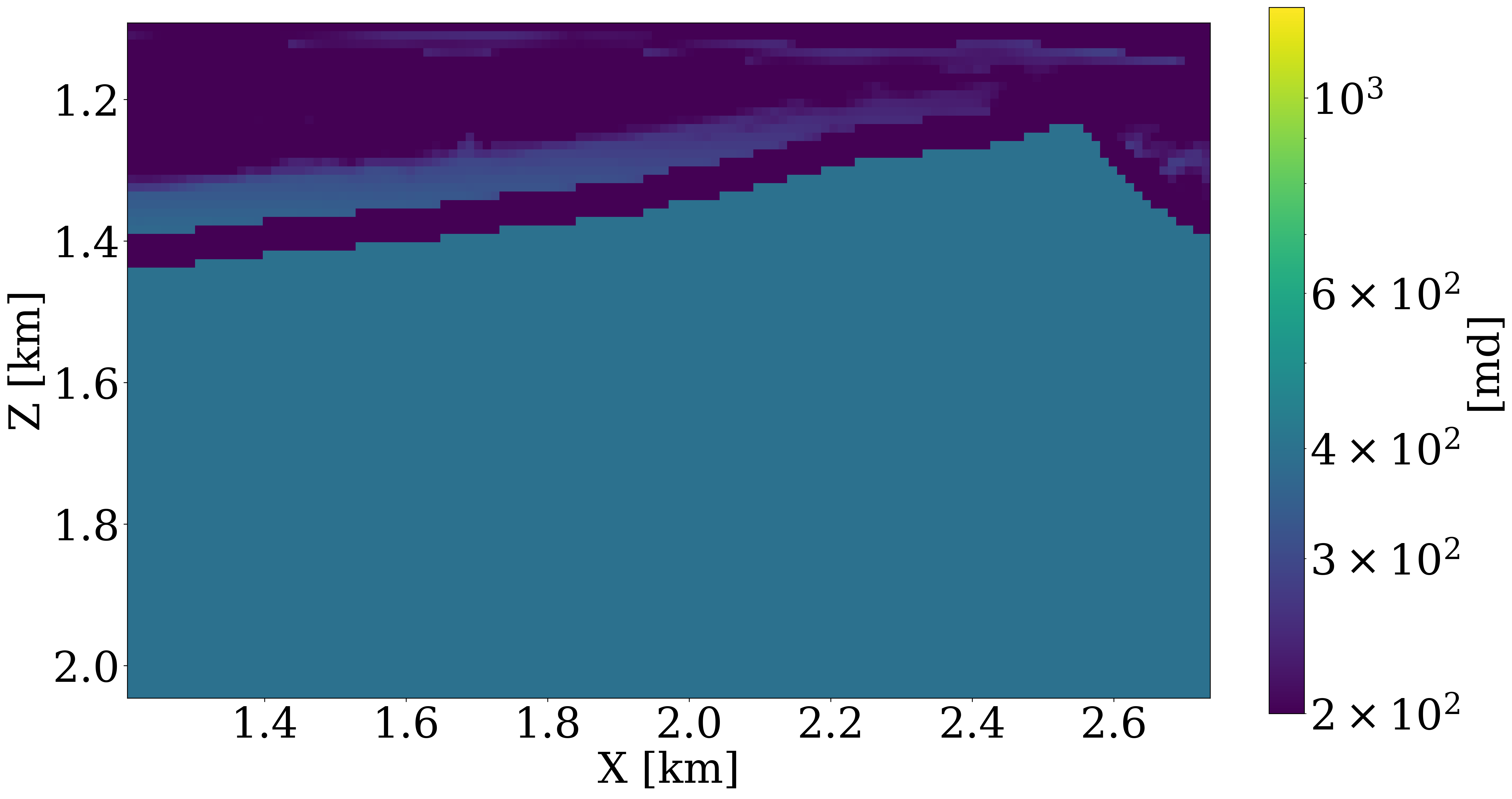
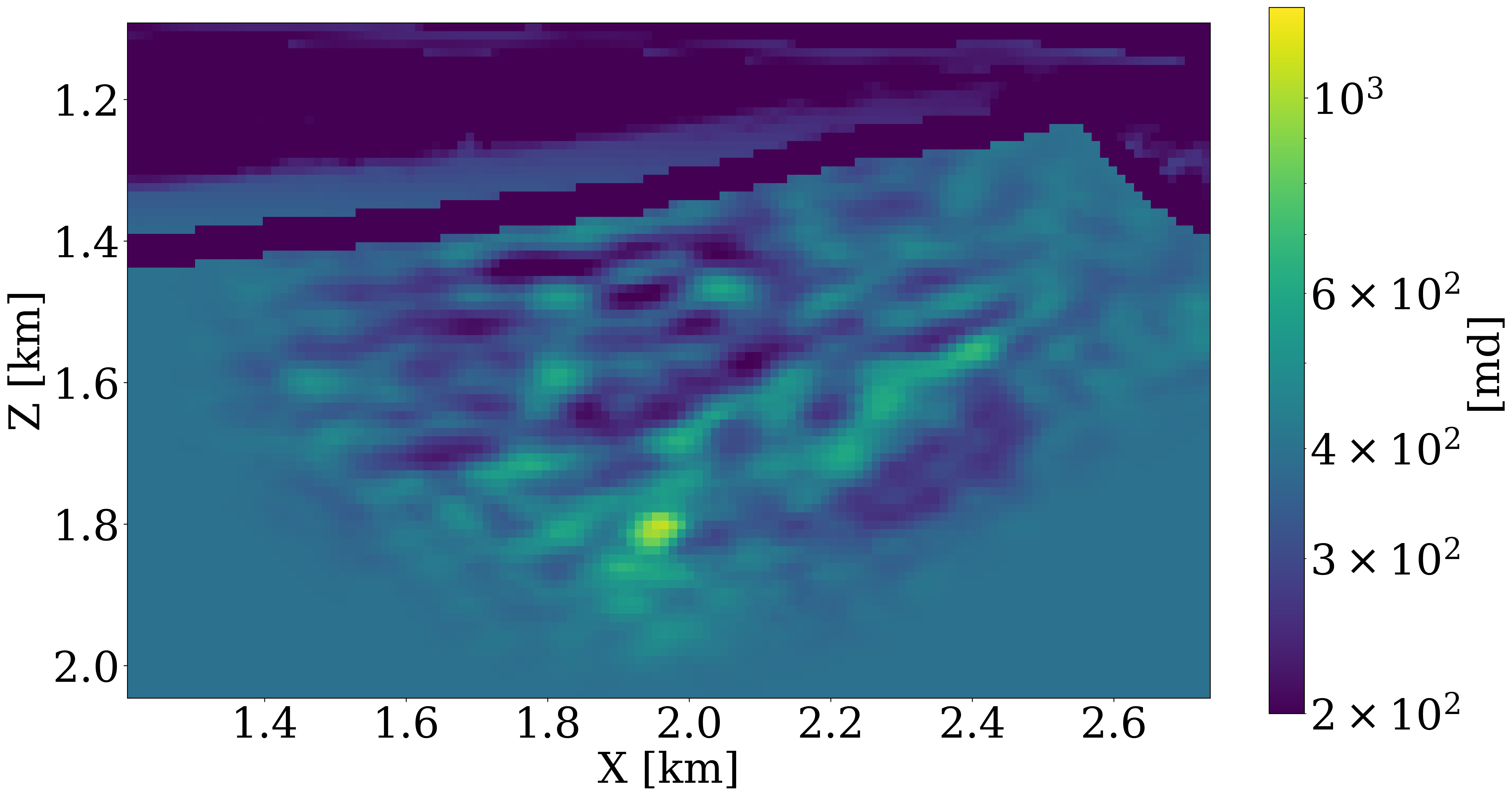
While initial results by Yin et al. (2022) were encouraging and showed strong benefits from the learned prior, the permeability model and fluid flow simulations considered in their study were too simplistic. To evaluate the proposed end-to-end inversion methodology in a more realistic setting, we consider the permeability model plotted in Figure 6 (a), which we derived from a slice of the Compass model (Jones et al. 2012) shown in Figure 2. To generate realistic CO2 plumes in this model, we generate immiscible and compressible two-phase flow simulations with JutulDarcy.jl over a period of 18 years with 5 snapshots plotted at years 10, 15, 16, 17, and 18. These CO2 snapshots are shown in the first row of Figure 7. Next, given the fluid-flow simulation, we use the patchy saturation model (Avseth, Mukerji, and Mavko 2010) to convert each CO2 concentration snapshot, \(\mathbf{c}^{i},\, i=1\ldots n_v\) to corresponding wavespeed model, \(\mathbf{v}^{i},\, i=1\ldots n_v\) with \(\mathbf{v}=\mathcal{R}(\mathbf{c})\). We then use JUDI.jl to generate synthetic time-lapse data, \(\mathbf{d}^{i},\, i=1\ldots n_v\), for each vintage.
During the inversion, the first 15 years of time-lapse data, \(\mathbf{d}^{i},\, i=1\ldots 15\), from the above synthetic experiment are inverted with permeabilities within the reservoir initialized by a single reasonable value as shown in Figure 6 (b). Inversion results obtained after 25 passes through the data for the physics-driven two-phase flow solver and its learned neural surrogate approximation are included in Figure 6 (c) and Figure 6 (d), respectively. Both results were obtained with 200 iterations of the code block shown above. Each time-lapse vintage consist of 960 receivers and 32 shots. To limit the number of wave-equation solves, gradients were calculated for only four randomly selected shots with replacement per iteration. While these results obtained without learned regularization are somewhat preliminary, they lead to the following observations. First, both inversion results for the permeability follow the inverted cone shape of the CO2. This is to be expected because permeability can only be inverted where CO2 has flown over the first 15 years. Second, the inverted permeability follows trends of this strongly heterogeneous model. Third, as expected details and continuity of the results obtained with the two-phase flow solver are better. In part, this can be explained by the fact that there are no guarantees that the model iterations remain with the statistical distribution on which the FNO was trained. Fourth, the implementation of this workflow greatly benefited from the software design principles listed above. For instance, the use of abstractions made it trivial to replace physics-driven two-phase flow solvers with their learned counterparts.
Despite the inversion results being preliminary, the 18 year CO2 simulations in both inverted permeability models are reasonable when comparing the true plume development plotted in the top row of Figure 7 with plumes simulated from the inverted models plotted in rows three and four of Figure 7. While certain details are missing in the estimates for the past, current, and predicted CO2 concentrations, the inversion constitutes a considerable improvement compared to plumes generated in the starting model for the permeability plotted in the second row of Figure 7. An early version of the presented workflow can be found in the Julia Package Seis4CCS.jl. As the project matures, updated workflows and codes will be pushed to GitHub.


Remaining challenges
So far, we hope we were able to convince the reader that working with abstractions certainly has its benefits. Thanks to the math-inspired abstractions, which naturally lead to modularity and separation of concerns, we were able to accelerate the research & development cycle for the end-to-end inversion. As a result, we created a development environment that allowed us to include machine learning techniques. Relatively late in the development cycle, it also gave us the opportunity to swap out the original 2D reservoir simulation code for a much more powerful and fully-featured industry-strength 3D code developed by a national lab. What we unfortunately not yet have been able to do is to demonstrate our ability to scale this end-to-end inversion to 3D, while both the Devito-based propagators and Jutul.jl’s fluid-flow simulations both have been demonstrated on industry-scale problems. Unfortunately, lack of access to large-scale computational resources makes it challenging in an academic environment to validate the proposed methodology on 4D synthetic and field data even though the computational toolchain presented in this paper is fully differentiable and in principle capable of scale-up. Most components have been separately tested and verified on realistic 3D examples (Grady et al. 2022; Møyner and Bruer 2023; Mathias Louboutin and Herrmann 2022; Mathias Louboutin and Herrmann 2023) and efforts are underway to remove fundamental memory and other bottlenecks.
Scale-up normalizing flows
Generative models, and NFs included, call for relatively large training sets and large computational resources for training. While efforts have been made to create training sets for the more traditional machine learning tasks, no public-domain training set exists that contains realistic 3D examples. The good news is that normalizing flows (Rezende and Mohamed 2015) have a small memory footprint compared to diffusion models (Song et al. 2020), so training this type of network will be feasible when training sets and compute become available. In our laboratory, we were already able to successfully train and evaluate NFs on \(256 \times 256 \times 64\) models.
Scale-up neural operators
Since the seminal paper by (Z. Li et al. 2020), there has been a flurry of publications on the use of FNOs as neural surrogates for expensive multiphase fluid-flow solvers used to simulate CO2 injection as part of geological storage projects (Wen et al. 2022, 2023). While there is good reason for this excitement, challenges remain when scaling this technique to realistic 3D problems. In that case, additional measures have to be taken. For instance, by nesting FNOs Wen et al. (2023) were able to divide 3D domains into smaller hierarchical subdomains centered around the wells, an approach that is only viable when certain assumptions are met. Because of this nested decomposition, these authors avoid the large memory footprint of 3D FNOs and report many orders of magnitude speedup. Given the potential impact of irregular CO2 flow, e.g., leakage, we as much as possible try to avoid making assumptions on the flow behavior and propose an accurate distributed Fourier neural operator (dfno) structure based on a domain decomposition of the network’s input and network weights (Grady et al. 2022). By using DistDL (Hewett and Grady II 2020), a software package that supports “model parallelism” in machine learning, our dfno partitions the input data and network weights across multiple GPUs such that each partition is able to fit in the memory of a single GPU. As reported by Grady et al. (2022), our work demonstrated validity of dfno on realistic problem and reasonable training set (permeability/CO2 concentration pairs) sizes, for permeability models derived from the Sleipner benchmark model (Furre et al. 2017). On 16 timesteps and models of size \(64 \times 118 \times 263\), we reported from our perspective a more realistic speedup of over \(1300\times\) compared to the simulation time on Open Porous Media (Rasmussen et al. 2021), one of the leading open-source reservoir simulators. These results confirm a similar indepedent approach advocated by P. A. Witte et al. (2022). Even though we are working with our industrial partners and Extreme Scale Solutions to further improve these numbers, we are confident that distributed FNOs are able to scale to 3D with a high degree of parallel efficiency.
Towards scalable open-source software
In addition to allowing for reproduction of published results, we are big advocates of pushing out scalable open-source software to help with the energy transition and with combating climate change. As observed in other fields, most notably in machine learning, open-source software leads to accelerated rates of innovation, a feature we need as an industry faced with major challenges. Despite the above exposition on our experiences implementing end-to-end permeability inversion, this work constitutes a snapshot of an ongoing project. However, many of the software components listed in Table 1 are in an advanced stage of development and to a large degree ready to be tested in 3D and ultimately on field data. For instance, all our software supports large-scale 3D simulation and AD. In addition, we are in advanced state of development to support GPU for all codes. For those curious on future developments, we also include below the Julia package ParametricOperators.jl, which is designed to allow for high-dimensional parallel tensor manipulations in support of future Julia-native implementations of distributed FNOs.
The work presented in this paper would not have been possible without open-source efforts from other groups, most notably by researchers at the UK’s Imperial College London who spearheaded the development of Devito and researchers at Norway’s SINTEF. By integrating these packages into Julia’s agile differentiable programming environment, we believe that we are well on our way to arrive at a software environment that is much more viable than the sum of its parts. We welcome readers to check https://github.com/slimgroup for the latest developments.
| Package | 3D | GPU | AD | Parallelism |
|---|---|---|---|---|
| Devito\(^*\) | yes | yes | no | domain-decomposition via MPI, multi-threading via OpenMP |
| JUDI.jl | yes | yes | yes | multi-threading via OpenMP, task parallel |
| JUDI4Cloud.jl | yes | yes | yes | multi-threading via OpenMP, task parallel |
| InvertibleNetworks.jl | yes | yes | yes | Julia-native multi-threading |
| dfno | yes | yes | yes | domain-decomposition via MPI |
| Jutul.jl\(^*\) | yes | soon | yes | Julia-native multi-threading |
| JutulDarcyRules.jl | yes | soon | yes | Julia-native multi-threading |
| Seis4CCS.jl | yes | yes | yes | Julia-native multi-threading |
| ParametricOperators.jl | yes | yes | yes | domain-decomposition via MPI, Julia-native multi-threading |
Conclusions
In this work, we introduced a software framework for geophysical inverse problems and machine learning that provides a scalable, portable, and interoperable environment for research and development at scale. We showed that through carefully chosen design principles, software with math-inspired abstractions can be created that naturally leads to desired modularity and separation of concerns without sacrificing performance. We achieve this by combining Devito’s automatic code generation for wave propagators with Julia’s modern highly performant and scalable programming capabilities, including differentiable programming. Thanks to these features, we were able to quickly implement a prototype, in principle scalable to 3D, for permeability inversion from time-lapse crosswell seismic data. Aside from the use of proper abstractions, our approach to solving this relatively complex multiphysics problem extensively relied on Julia’s innate algorithmic differentiation capabilities, supplemented by auxiliary performant derivatives for the wave/fluid-flow physics, and for components of the machine learning. On account of these design choices, we developed an agile and relatively easy to maintain compact software stack where low-level code is hidden through a combination of math-inspired abstractions, modern programming practices, and automatic code generation.
Code and data availability
Our software framework is organized into registered Julia packages, all of which can be found on the SLIM GitHub page (https://github.com/slimgroup). The software packages described in this paper are all open-source and released under the MIT license for use by the community.
Acknowledgment
This research was carried out with the support of Georgia Research Alliance and industrial partners of the ML4Seismic Center. The authors thank Henryk Modzelewski (University of British Columbia) and Rishi Khan (Extreme Scale Solutions) for constructive discussions. This work was supported in part by the US National Science Foundation grant OAC 2203821 and the Department of Energy grant No. DE-SC0021515.