De-risking geological carbon storage from high resolution time-lapse seismic to explainable leakage detection

Ziyi Yin, Huseyin Tuna Erdinc, Abhinav Prakash Gahlot, Mathias Louboutin, Felix J. Herrmann
Georgia Institute of Technology

Introduction

For various reasons, seismic monitoring of geological carbon storage (GCS) comes with its own set of unique challenges. Amongst these challenges, the need for low-cost highly repeatable, high resolution, and high fidelity images ranks chiefly. While densely sampled and replicated time-lapse surveys—which rely on permanent reservoir monitoring systems—may be able to provide images conducive to interpretation and reservoir management, these approaches are often too costly and require too much handholding to be of practical use for GCS.

To overcome these challenges, we replace the current paradigm of costly replicated acquisition, cumbersome time-lapse processing, and interpretation, by a joint inversion framework mapping time-lapse data to high fidelity and high resolution images from sparse non-replicated time-lapse surveys. We demonstrate that we arrive at an imaging framework that is suitable for automatic detection of pressure-induced CO₂ leakage. Rather than relying on meticulous 4D workflows where baseline and monitoring surveys are processed separately to yield accurate and artifact-free time-lapse differences, our approach exposes information that is shared amongst the different vintages by formulating the imaging problem in terms of an unknown fictitious common component, and innovations of the baseline and monitor survey(s) with respect to this common component. Because the common component is informed by all time-lapse surveys, its image quality improves when the surveys bring complementary information, which is the case when the surveys are not replicated. In turn, the enhanced common component results in improved images for the baseline, monitor, and their time-lapse difference. Joint inversion also leads to robustness with respect to noise, calibration errors, and time-lapse changes in the background velocity model.

To showcase the achievable imaging gains and how these can be used in a GCS setting where CO₂ leakage is of major consideration, we create hundreds of time-lapse imaging experiments involving CO₂ plumes whose behavior is determined by the two-phase flow equations. To mimic irregular flow due to pressure-induced opening of fractures, we increase the permeability in the seal at random locations and pressure thresholds. The resulting flow simulations are used to generate time-lapse datasets that serve as input to our joint imaging scheme. The produced time-lapse difference images are subsequently used to train and test a neural network that as an explainable classifier determines whether the CO₂ plume behaves regularly or shows signs of leakage.

Our contributions are organized as follows. First, we discuss the time-lapse seismic imaging problem and its practical difficulties. Next, we introduce the joint recovery model that takes explicit advantage of information shared by multiple surveys. By means of a carefully designed synthetic case study involving saline aquifers made of Blunt sandstone in the Southern North Sea, we demonstrate the uplift of the joint recovery model and how its images can be used to train a deep neural network classifier to detect erroneous growth of the CO₂ plume automatically. Aside from determining whether the CO₂ plume behaves regularly or not, our network also provides class activation mappings that visualize areas in the image on which the network is basing its classification.

Seismic monitoring with time-lapse imaging

To keep track of CO₂ plume development during geological carbon storage (GCS) projects, multiple time-lapse surveys are collected. Baseline surveys are acquired before the supercritical CO₂ is injected into the reservoir. These baseline surveys, denoted by the index \(j=1\), are followed by one or more monitor surveys, collected at later times and indexed by \(j=2,\cdots,n_v\) with \(n_v\) the total number of surveys.

Seismic monitoring of GCS brings its own unique set of challenges that stem from the fact that its main concern is (early) detection of possible leakage of CO₂ from the storage complex. To be successful with this task, monitoring GCS calls for a time-lapse imaging modality that is capable of

• detecting weak time-lapse signals associated with small rock-physics changes induced by CO₂ leakage
• attaining high lateral resolution from active-source surface seismic data to detect vertically moving leakage
• handling an increasing number of seismic surveys collected over long periods of time (\(\sim50-100\) years)
• reducing costs drastically by no longer insisting on replication of time-lapse surveys to attain high degrees of repeatability
• lowering the cumulative environmental imprint of active source acquisition

Monitoring with the joint recovery model

To meet these challenges, we choose a linear imaging framework where observed linearized data for each vintage is related to perturbations in the acoustic impedance via \[ \begin{equation} \mathbf{b}_j=\mathbf{A}_j\mathbf{x}_j+\mathbf{e}_j\quad \text{for}\quad j=1,2,\cdots,n_v. \label{eq-lin-model} \end{equation} \] In this expression, the matrix \(\mathbf{A}_j\) stands for the linearized Born scattering operator for the \(j\,\mathrm{th}\) vintage. Observed linearized data, collected for all shots in the vector \(\mathbf{b}_j\), is generated by applying the \(\mathbf{A}_j\)’s to the (unknown) impedance perturbations denoted by \(\mathbf{x}_j\) for \(j=1,2,\cdots, n_v\). The task of time-lapse imaging is to create high resolution, high fidelity and true amplitude estimates for the time-lapse images, \(\left\{\widehat{\mathbf{x}}_j\right\}_{j=1}^{n_v}\), from non-replicated sparsely sampled noisy time-lapse data.

We argue that our choice for linearized imaging is justified for four reasons. First, CO₂-injection sites undergo extensive baseline studies, which means that accurate information on the background velocity model is generally available. Second, changes in the acoustic parameters induced by CO₂ injection are typically small, so it suffices to work with one and the same background model for the baseline and monitor surveys. Third, when the background model is sufficiently close to the true model, linearized inversion, which corresponds to a single Gauss-Newton iteration of full-waveform inversion, converges quadratically. Fourth, because the forward model is linear, it is conducive to the use of the joint recovery model where inversions are carried out with respect to the common component, which is shared between all vintages, and innovations with respect to the common component. Because the common component represents an average, we expect this joint imaging method to be relatively robust with respect to kinematic changes induced by time-lapse effects or by lack of calibration of the acquisition (Oghenekohwo and Herrmann, 2017a).

By parameterizing time-lapse images, \(\left\{\mathbf{x}_j\right\}_{j=1}^{n_v}\), in terms of the common component, \(\mathbf{z}_0\), and innovations with respect to the common component, \(\left\{\mathbf{z}_j\right\}_{j=1}^{n_v}\), we arrive at the joint recovery model where representations for the images are given by \[ \begin{equation} \mathbf{x}_j = \frac{1}{\gamma}\mathbf{z}_0 + \mathbf{z}_j \quad \text{for} \quad j=1,2,\cdots,n_v. \label{eq-components} \end{equation} \] Here, the parameter, \(\gamma\), controls the balance between the common component, \(\mathbf{z}_0\), and innovation components, \(\left\{\mathbf{z}_j\right\}_{j=1}^{n_v}\) (X. Li, 2015). Compared to traditional time-lapse approaches, where data are imaged separately or where time-lapse surveys are subtracted, inversions for time-lapse images based on the above parameterization are carried out jointly and involve inverting the following matrix: \[ \begin{equation} \begin{aligned} \mathbf{A} = \begin{bmatrix} \frac{1}{\gamma} \mathbf{A}_1 & \mathbf{A}_1 & & \\ \vdots & & \ddots & \\ \frac{1}{\gamma} \mathbf{A}_{n_v} & & & \mathbf{A}_{n_v} \end{bmatrix}. \end{aligned} \label{eq-jrm} \end{equation} \] While traditional time-lapse imaging approaches strive towards maximal replication between the surveys to suppress acquisition related artifacts, imaging with the joint recovery model—which entails inverting the underdetermined system in Equation \(\ref{eq-jrm}\) using structure-promotion techniques (e.g. via \(\ell_1\)-norm minimization)—improves the image quality of the vintages themselves in situations where the surveys are not replicated. This occurs in cases where \(\mathbf{A}_i\neq\mathbf{A}_j\) for \(\forall i\neq j\), or in situations where there is significant noise. This remarkable result was shown to hold for sparsity-promoting denoising of time-lapse field data (Wei et al., 2018; Tian et al., 2018), for various wavefield reconstructions of randomized simultaneous-source dynamic (towed-array) and static (OBC/OBN) marine acquisitions (Oghenekohwo and Herrmann, 2017a; Kotsi, 2020; W. Zhou and Lumley, 2021), and for wave-based inversion, including least-squares reverse-time migration and full-waveform inversion (Oghenekohwo, 2017; Oghenekohwo and Herrmann, 2017b). The observed quality gains in these applications can be explained by improvements in the common component resulting from complementary information residing in non-replicated time-lapse surveys. This enhanced recovery of the common component in turn improves the recovery of the innovations and therefore the vintages themselves. The time-lapse differences themselves also improve, or at the very least, remain relatively unaffected when the surveys are not replicated. Relaxing replication of surveys obviously leads to reduction in cost and environmental impact. Below, we show how GCS monitoring also benefits from this approach.

Monitoring with curvelet-domain structure promotion

To obtain high resolution and high fidelity time-lapse images, we invert the system in Equation \(\ref{eq-jrm}\) (M. Yang et al., 2020; Witte et al., 2019b; Z. Yin et al., 2021) with \[ \begin{equation} \begin{split} \underset{\mathbf{z}}{\operatorname{minimize}} \quad \lambda \|\mathbf{C}\mathbf{z}\|_1+\frac{1}{2}\|\mathbf{C}\mathbf{z}\|_2^2 \\ \text{subject to}\quad \|\mathbf{b}- \mathbf{A}\mathbf{z}\|_2^2 \leq \sigma, \end{split} \label{eq-elastic} \end{equation} \] where \(\mathbf{C}\) is the forward curvelet transform, \(\lambda\) the threshold parameter, and \(\sigma\) the magnitude of the noise. At iteration \(k\) and for \(\sigma=0\), solving Equation \(\ref{eq-elastic}\) corresponds to computing the following iterations: \[ \begin{equation} \begin{aligned} \begin{array}{lcl} \mathbf{u}_{k+1} & = & \mathbf{u}_k-t_k \mathbf{A}_k^\top(\mathbf{A}_k\mathbf{z}_{k}-\mathbf{b}_k)\\ \mathbf{z}_{k+1} & = & \mathbf{C}^\top S_{\lambda}(\mathbf{C}\mathbf{u}_{k+1}), \end{array} \end{aligned} \label{LBk} \end{equation} \] where \(\mathbf{A}_k\), with a slight abuse of notation, represents the matrix in Equation \(\ref{eq-jrm}\) for a subset of shots randomly selected from sources in each survey. The vector \(\mathbf{b}_k\) contains the extracted shot records from \(\mathbf{b}\) and the symbol \(^\top\) refers to the adjoint. Sparsity is promoted via curvelet-domain soft thresholding, \(S_{\lambda}(\cdot)=\max(|\cdot|-\lambda,0)\operatorname{sign}(\cdot)\), where, \(\lambda\), is the threshold. The vectors \(\mathbf{u}_k\) and \(\mathbf{z}_k\) contain the baseline and innovation components.

Numerical case study: Blunt sandstone in the Southern North Sea

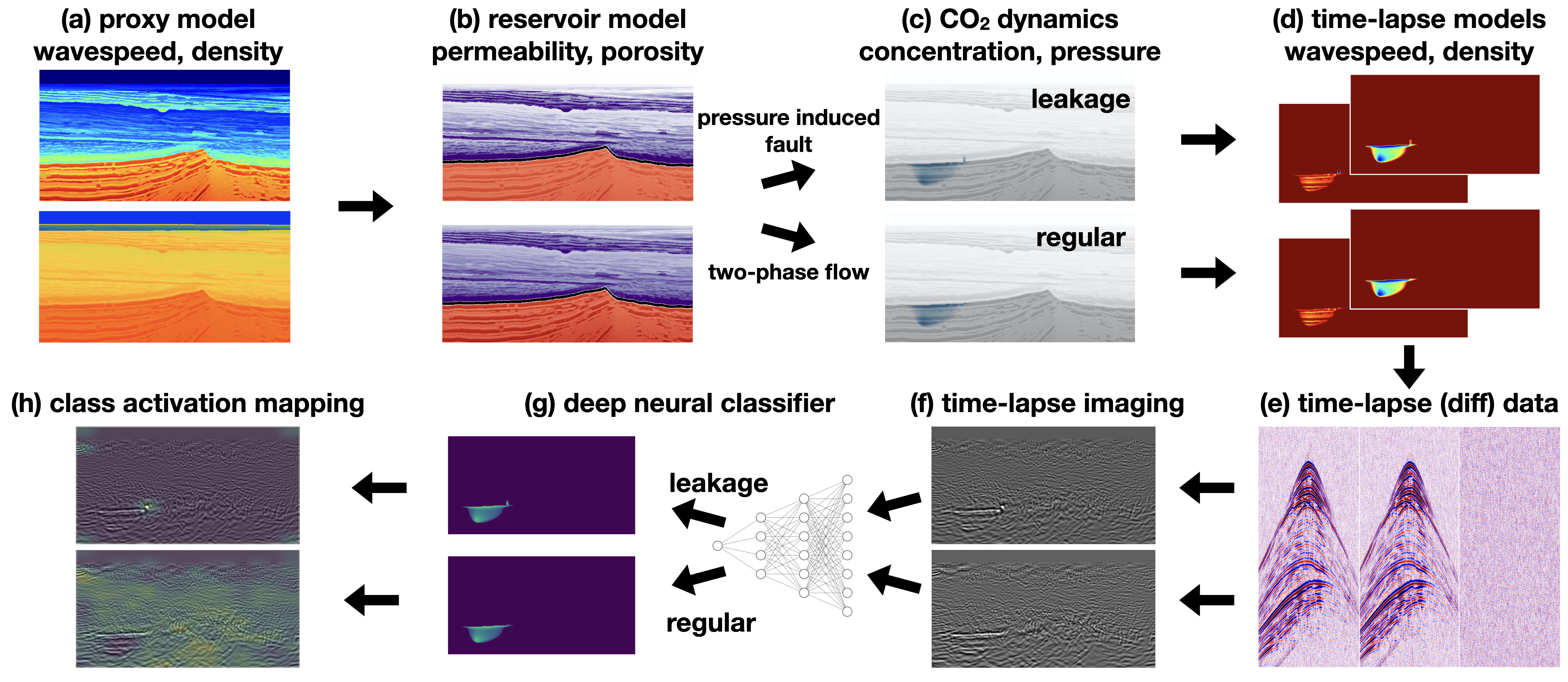
Before discussing the impact of high resolution and high fidelity time-lapse imaging with the joint recovery model on the down-stream task of automatic leakage detection with a neural network classifier, we first detail the setup of our numerical experiments using techniques from simulation-based acquisition design as described by Z. Yin et al. (2021). In order to generate realistic time-lapse data and training sets for the automatic leakage classifier, we follow the workflow summarized in Figure 1. In this approach, use is made of proxy models for seismic properties derived from real 3D imaged seismic and well data (C. Jones et al., 2012). With rock physics, these seismic models are converted to fluid-flow models that serve as input to two-phase flow simulations. The resulting datasets, which include pressure-induced leakage, will be used to create time-lapse data used to train our classifier. For more detail, refer to the caption of Figure 1.

Proxy seismic and fluid-flow models

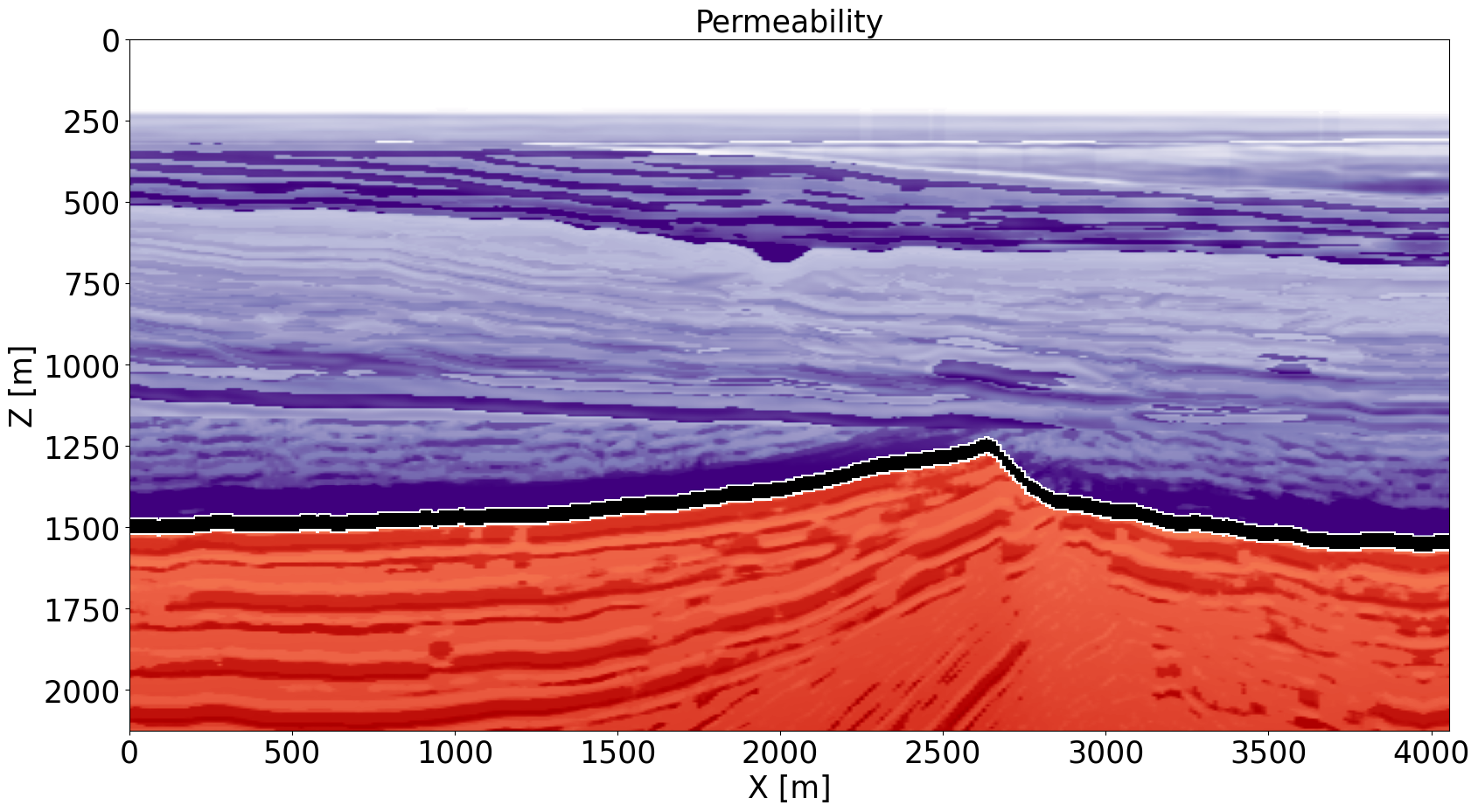
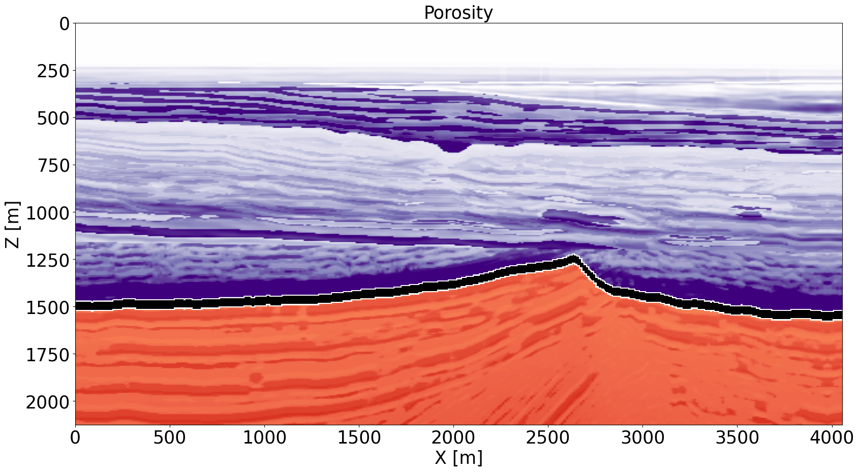
Amongst the various CO₂ injection projects, GCS in offshore saline aquifers has been most successful in reaching scale and in meeting injection targets. For that reason, we consider a proxy model constructed representative for CO₂ injection in the South of the North Sea involving a saline aquifer made of the highly permeable Blunt sandstone. This area, which is actively being considered for GCS (Kolster et al., 2018), consists of the following three geologic sections (see Figure 2 for the permeability and porosity distribution):

1. the highly porous (average \(33\%\)) and permeable (\(>170\,\mathrm{mD}\)) Blunt sandstone reservoir of about \(300-500\,\mathrm{m}\) thick. This section, denoted by red colors in Figure 2, corresponds to the saline aquifer and serves as the reservoir for CO₂ injection;

2. the primary seal (permeability \(10^{-4}-10^{-2}\,\mathrm{mD}\)) made of the Rot Halite Member, which is \(50\,\mathrm{m}\) thick and continuous (black layer in Figure 2);

3. the secondary seal made of the Haisborough group, which is \(>300\,\mathrm{m}\) thick and consists of low-permeable (permeability \(15-18\,\mathrm{mD}\)) mudstone (purple section in Figure 2).

To arrive at the fluid-flow models, we consider 2D subsets of the 3D Compass model (C. Jones et al., 2012) and convert these seismic models to fluid-flow properties (see Figure 1 (b)) by assuming a linear relationship between compressional wavespeed and permeability in each stratigraphic section. For further details on the conversion of compressional wavespeed and density to permeability and porosity, we refer to empirical relationships reported in Klimentos (1991). During conversion, an increase of \(1\mathrm{km/s}\) in compressional wavespeed is assumed to correspond to an increase of \(1.63\,\mathrm{mD}\) in permeability. From this, porosity is calculated with the Kozeny-Carman equation (A. Costa, 2006) \(K = \mathbf{\phi}^3 \left(\frac{1.527}{0.0314*(1-\mathbf{\phi})}\right)^2\), where \(K\) and \(\phi\) denote permeability (\(\mathrm{mD}\)) and porosity (%) with constants taken from the Strategic UK CCS Storage Appraisal Project report.

Fluid-flow simulations

To model CO₂ plumes that behave regularly and irregularly, the latter due to leakage, we solve the two-phase flow equations numerically¹ for both pressure and concentration (D. Li and Xu, 2021; D. Li et al., 2020). To mimic possible pressure-induced CO₂ leakage, we increase the permeability at random distances away from the injection well within the seal from \(10^{-4}\,\mathrm{mD}\) to \(500\,\mathrm{mD}\) when the pressure exceeds \(\sim 15\,\mathrm{MPa}\). At that depth, the pressure is below the fracture gradient (Ringrose, 2020). Since pressure-induced fractures come in different sizes, we also randomly vary the width of the pressure-induced fracture openings from \(12.5\,\mathrm{m}\) to \(62.5\,\mathrm{m}\). Examples of fluid-flow simulations without and with leakage are shown in Figure 1 (c).

Rock-physics conversion

To monitor temporal variations in the plume’s CO₂ concentration seismically, we use the patchy saturation model (Avseth et al., 2010) to convert the CO₂ concentration to decrease in compressional wavespeed and density. These changes are shown in Figure 1 from (d). The fact that these induced changes in the time-lapse differences in seismic properties are relatively small in spatial extent (\(\sim 800\,\mathrm{m}\) for the plume and \(< 62.5 \,\mathrm{m}\) for the leakage) and amplitude (\(18\%\) of the impedance perturbations with respect to the background model) calls for a time-lapse imaging modality with small normalized root-mean-square (NRMS) (Kragh and Christie, 2002) values \((\sim 2.5\%)\). This NMRS value is based on the relative amplitude of impedance perturbations with respect to the background model ( \(14\%\)).

Time-lapse seismic simulations

To train and validate automatic detection of CO₂ leakage from the storage complex requires the creation of realistic time-lapse datasets that contain the seismic imprint of regular as well as irregular (leakage) plume development. To this end, baseline surveys are simulated prior to CO₂ injection for different subsets of the Compass model. Monitor surveys are simulated \(200\) days after leakage occurs to verify that potential leakage can be detected automatically early on. For regular plume development, we shoot monitor surveys for each subset at random times after CO₂ injection. In order to strike a balance between acquisition productivity and time-lapse image quality, use is made of dense permanent acoustic monitoring at the seafloor with \(25\,\mathrm{m}\) receiver spacing. Time-lapse acquisition costs are reduced by non-replicated coarse shooting with the source towed at \(10\,\mathrm{m}\) depth below the ocean surface. Subsampling artifacts are reduced by using a randomized technique from compressive sensing where \(32\) sources are located at non-replicated jittered (Herrmann and Hennenfent, 2008) source positions, yielding an average source sampling of \(125\,\mathrm{m}\). Given this acquisition geometry, linear data is generated² with Equation \(\ref{eq-lin-model}\) for a \(25\,\mathrm{Hz}\) Ricker wavelet and with the band-limited noise term set so that the data’s signal-to-noise ratio (SNR) is \(8.0\,\mathrm{dB}\). This noise level leads to an extremely poor SNR of \(-31.4\,\mathrm{dB}\) for time-lapse differences in the shot domain. See Figure 1 (e).

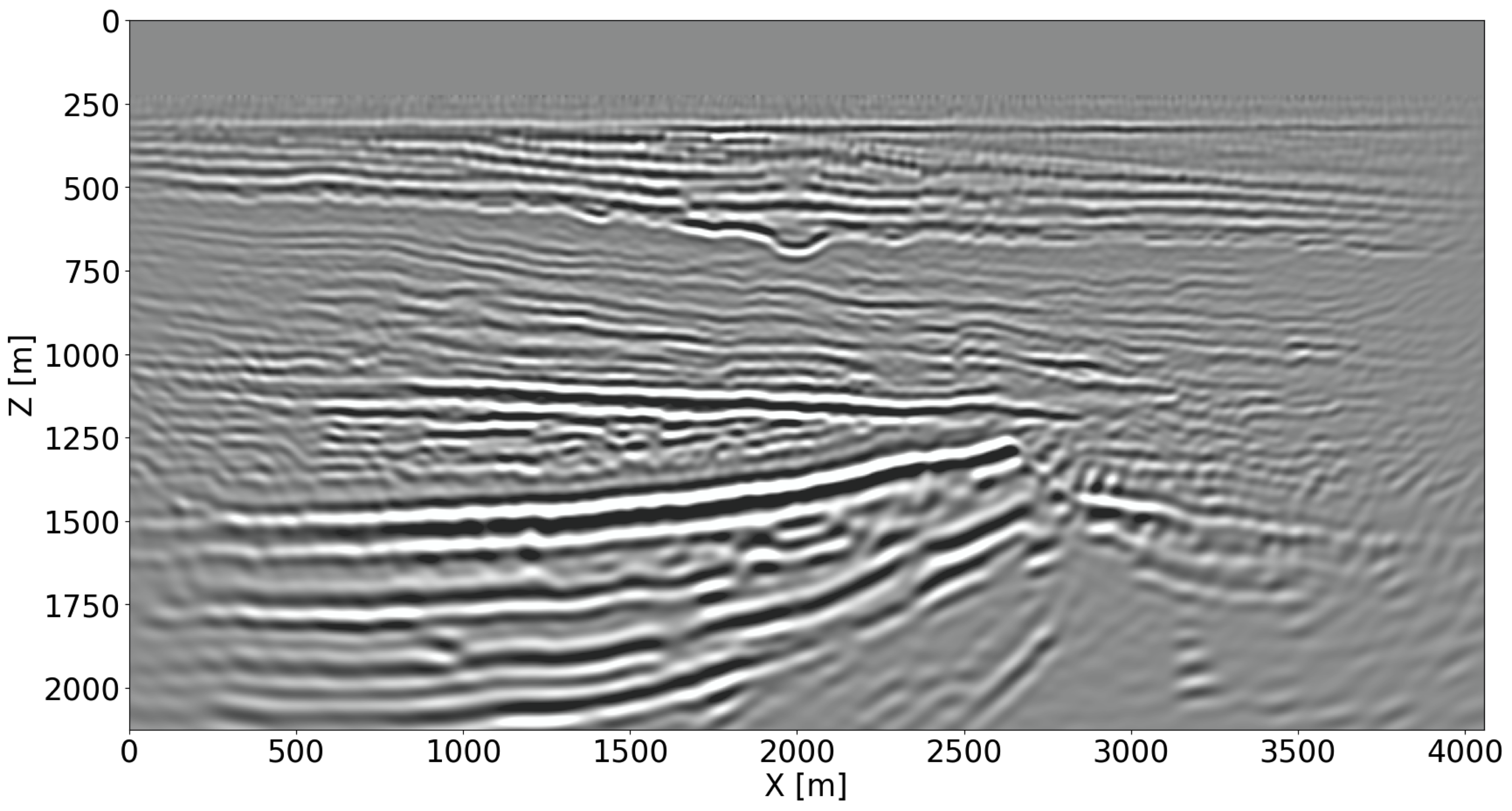
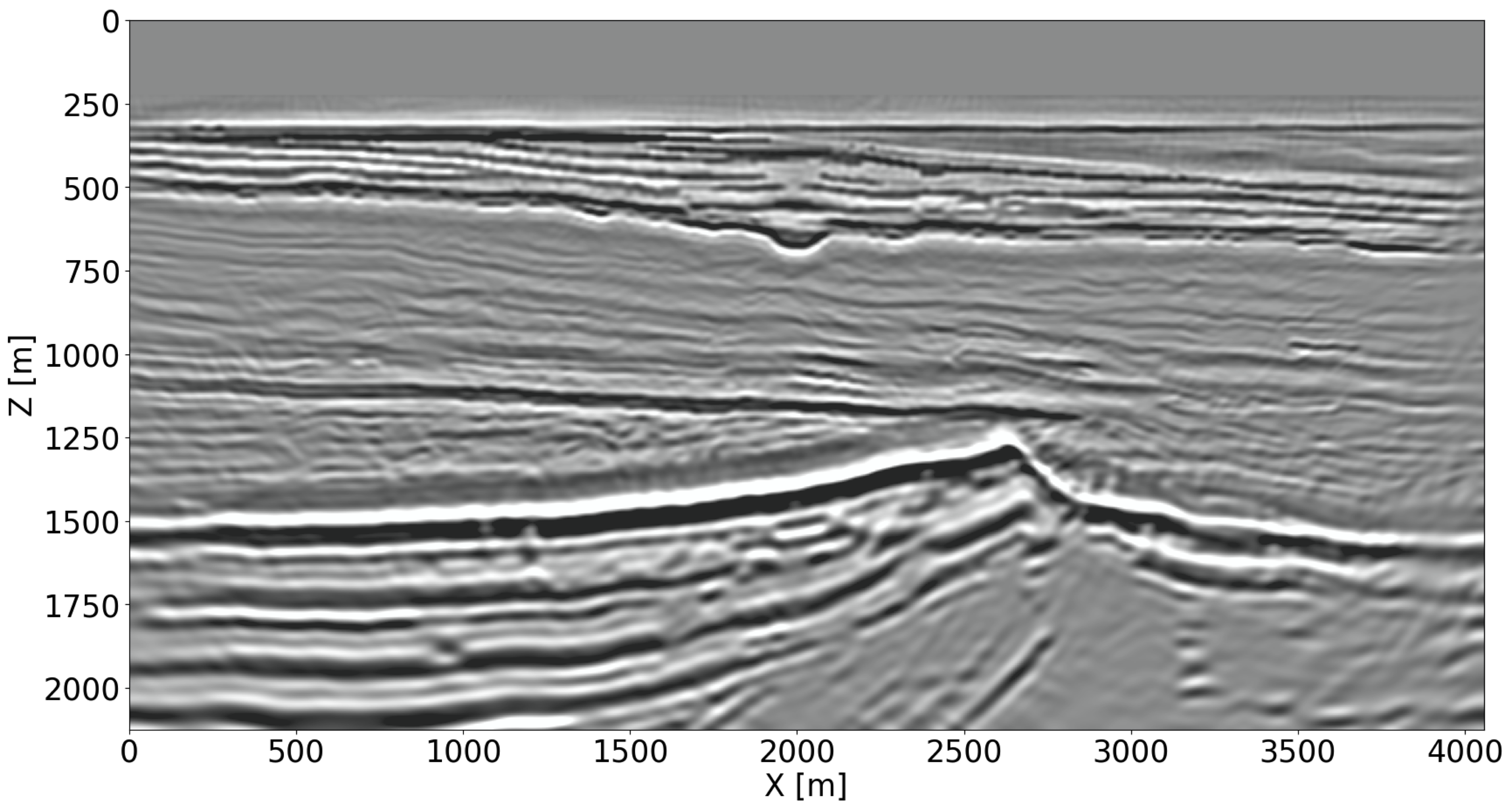
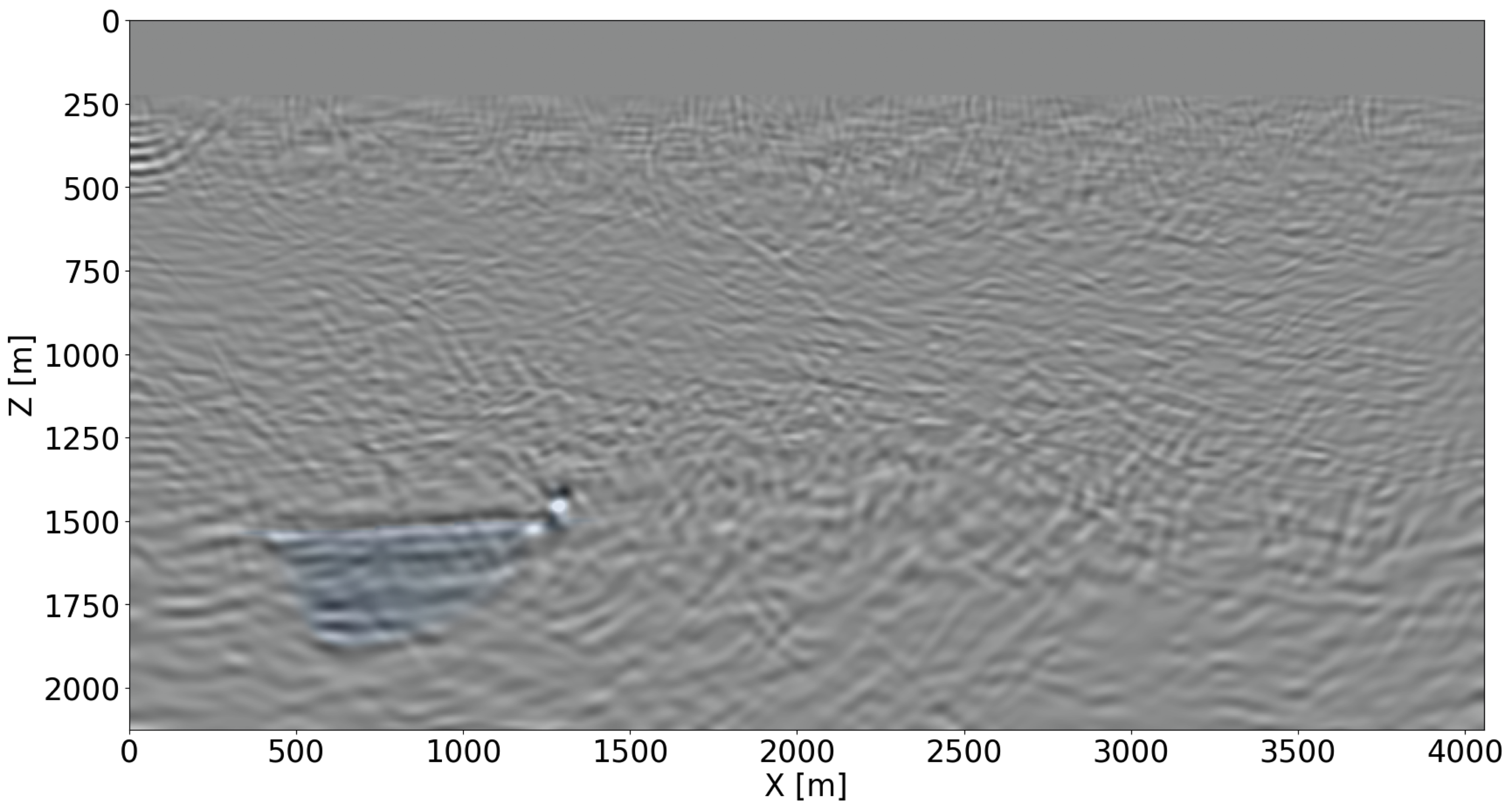
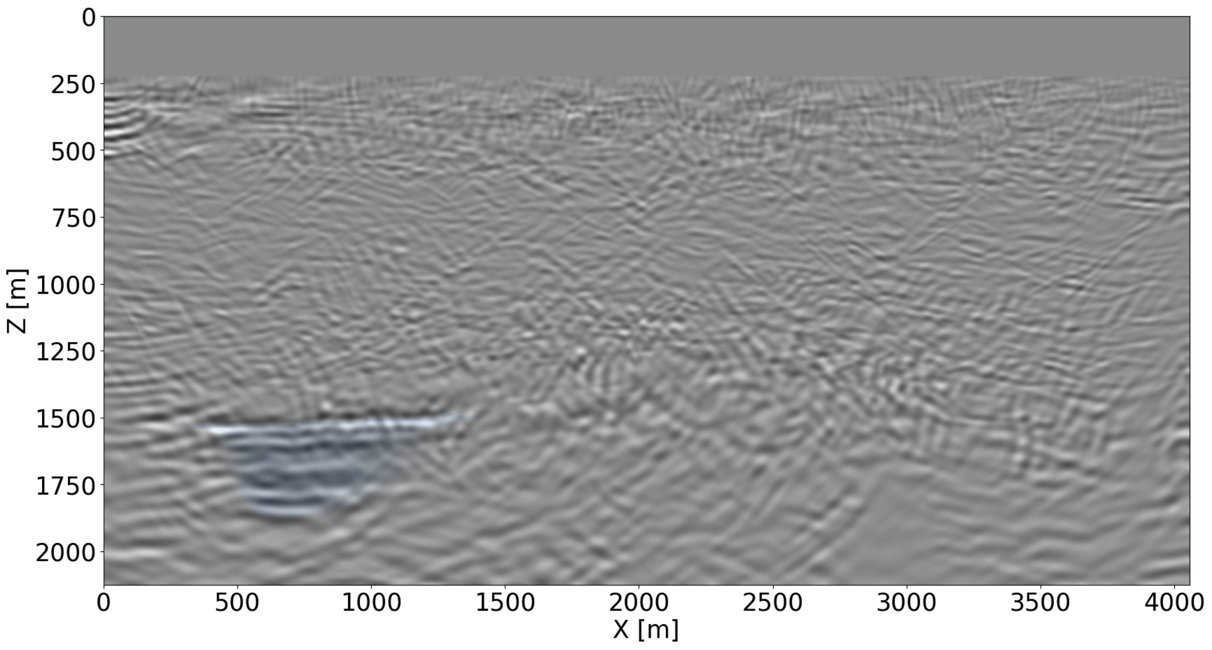
Imaging with joint recovery model versus reverse-time migration

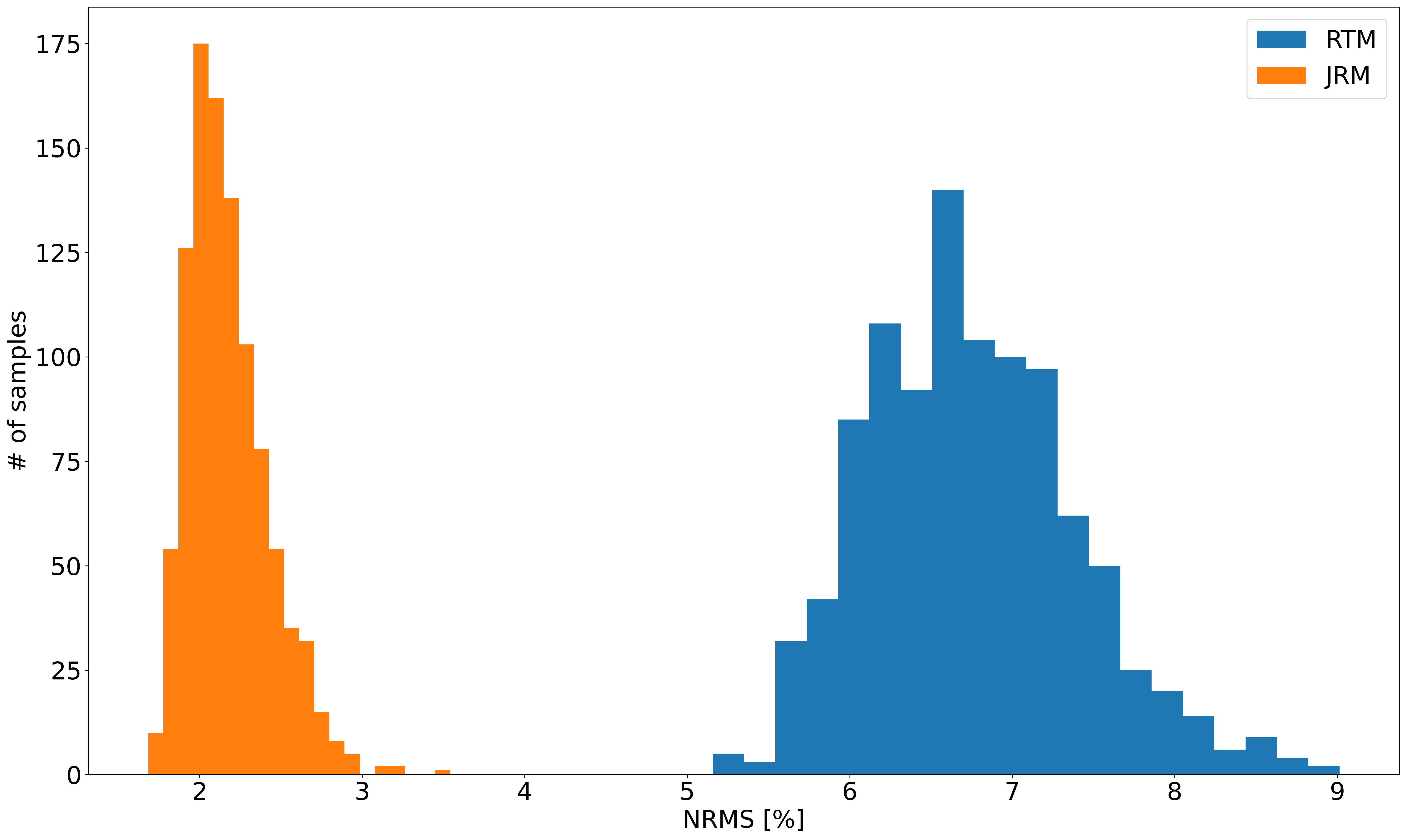
Given the simulated time-lapse datasets with and without leakage, time-lapse difference images are created according to two different imaging scenarios, namely via independent reverse-time migration (RTM), conducted on the baseline and monitor surveys separately, and via inversion of the joint recovery model (cf. Equations \(\ref{eq-jrm}\) and \(\ref{eq-elastic}\)). To limit the computational cost of the Bregman iterations (Equation \(\ref{LBk}\)), four shot records are selected per iteration at random from each survey for imaging (W. Yin et al., 2008; Witte et al., 2019b; M. Yang et al., 2020; Z. Yin et al., 2021), limiting the cost of the joint inversion to three RTMs. The recovered baseline images are shown in Figures 3a for RTM and 3b for JRM. For the leakage scenario, the time-lapse differences are plotted in Figures 3c and 3d, for RTM and JRM respectively. For the regular plume, the time-lapse differences are plotted in Figures 3e and 3f, for RTM and JRM respectively. From these images, it is clear that joint inversion leads to relatively artifact-free recovery of the vintages and time-lapse differences. This observation is reflected in the NRMS values, which improve considerably as shown by the histograms in Figure 4 for \(1000\) imaging experiments. Not only do the NRMS values shift towards the left, their values are also more concentrated when inverting time-lapse data with the joint recovery model. Both features are beneficial to automatic leakage detection.

Deep neural network classifier for CO₂ leakage detection

The injection of supercritical CO₂ into the storage complex perturbs the physical, chemical and thermal environment of the reservoir (Newell and Ilgen, 2019). Because CO₂ injection increases the pressure, this process may trigger CO₂ leakage across the seal when the pressure increase induces opening of pre-existing faults or fractures zones (Pruess, 2006; Ringrose, 2020). To ensure safe operations of CO₂ storage, we develop a quantitative leakage detection tool based on a deep neural classifier. This classifier is trained on time-lapse images that contain the imprint of CO₂ plumes that behave regularly and irregularly. In case of irregular flow, CO₂ escapes the storage complex through a pressure induced opening in the seal, which causes a localized increase in permeability (shown in Figure 3d).

Because time-lapse differences are small in amplitude, and strongly localized laterally when leakage occurs, highly sensitive learned classifiers are needed. For this purpose, we follow Erdinc et al. (2022) and adopt the Vision Transformer (ViT) (Dosovitskiy et al., 2020). This state-of-the-art classifier originated from the field of natural language processing (NLP) (Vaswani et al., 2017). Thanks to their attention mechanism, ViTs have been shown to achieve superior performance on image classification tasks where image patches are considered as word tokens by the transformer network. As a result, ViTs have much less image-specific inductive bias compared to convolutional neural networks (Dosovitskiy et al., 2020).

To arrive at a practical and performant ViT classifier, we start from a ViT that is pre-trained on image tasks with \(16\times 16\) patches and apply transfer learning (Yosinski et al., 2014) to fine-tune this network on \(1576\) labeled time-lapse images. Catastrophic forgetting is avoided by freezing the initial layers, which are responsible for feature extraction, during the initial training. After the initial training of the last dense layers, all network weights are updated for several epochs while keeping the learning rate small. The labeled (regular vs. irregular flow) training set itself consists of \(1576\) time-lapse datasets divided equally between regular and irregular flow.

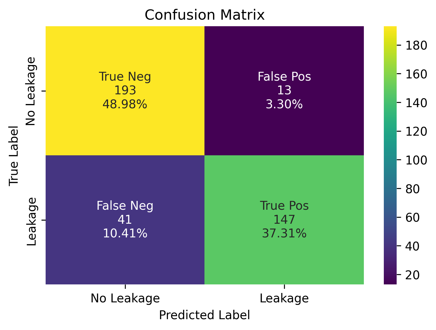
After the training is completed, baseline and monitor surveys are simulated for \(394\) unseen Earth models with regular and irregular plumes. These simulated time-lapse datasets are imaged with JRM by inverting the matrix in Equation \(\ref{eq-jrm}\) via Bregman iterations in Equation \(\ref{LBk}\). The resulting time-lapse difference images (see Figures 3d and 3f for two examples) serve as input to the ViT classifier. Refer to Figure 5 for performance, which corresponds to a two by two confusion matrix. The first row denotes the classification results for samples with regular plume (negative samples), where \(193\) (true negative) out of \(206\) samples are classified correctly. The second row denotes the classification results for samples with CO₂ leakage over the seal (positive samples), where \(147\) (true positive) out of \(188\) samples are classified correctly. Due to the fact that JRM recovers relatively artifact-free time-lapse differences, the classifier does not pick up too many artifacts related to finite acquisition as CO₂ leakage. This leads to much fewer false alarms for CO₂ leakage.

Class activation mapping based saliency map

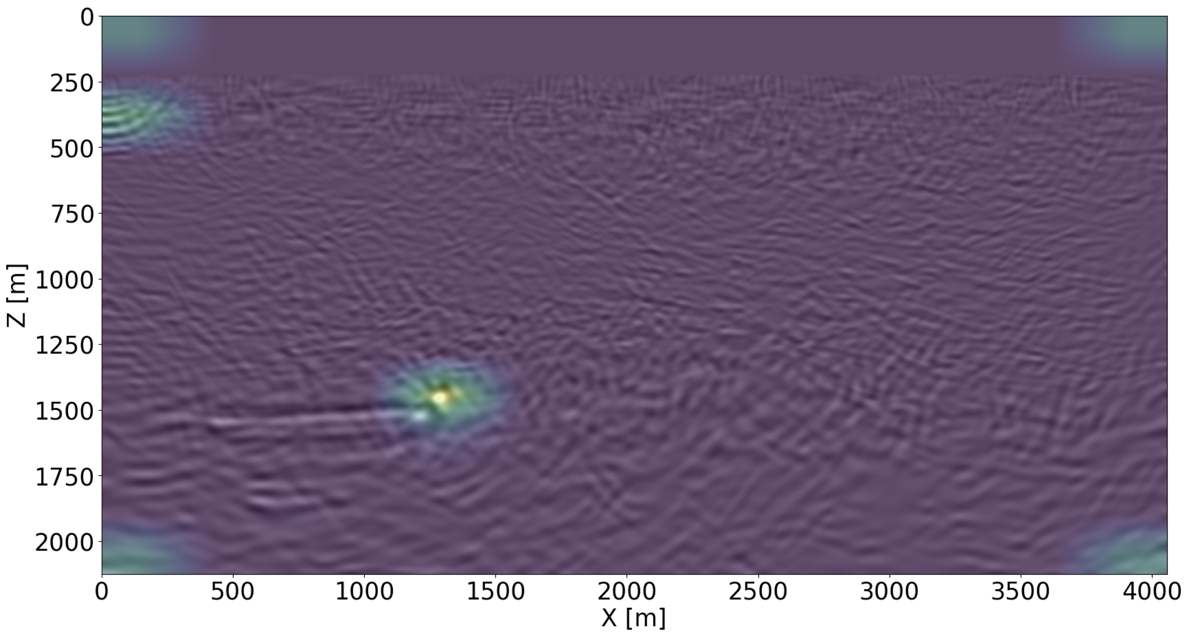
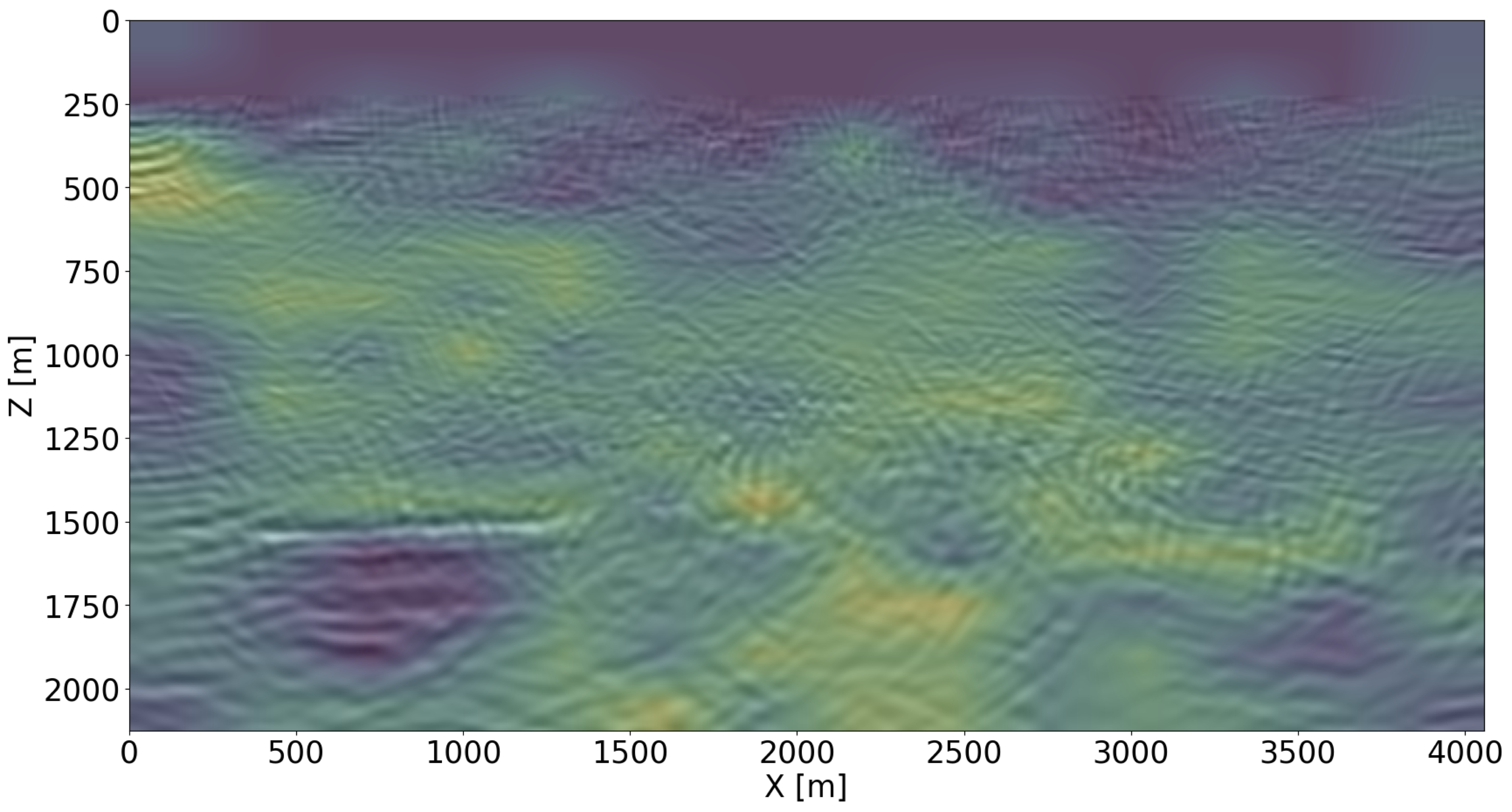
While our ViT classifier is capable of achieving good performance (see Figure 5), making intervention decisions during GCS projects calls for interpretability and trustworthiness of our classifier (Hooker et al., 2019; Y. Zhang et al., 2021; Mackowiak et al., 2021). To enhance these features, we take advantage of class activation mappings (CAM) (B. Zhou et al., 2016). These saliency maps help us to identify the discriminative spatial regions in each image that support a particular class decision. In our application, these regions correspond to areas where the classifier deems the CO₂ plume to behave irregularly (if the classification result is leakage). By overlaying time-lapse difference images with these maps, interpretation is facilitated, assisting practitioners to make decisions on how to proceed with GCS projects and take associated actions. Figure 6 illustrates how the Score CAM approach (H. Wang et al., 2020) serves this purpose³. Figure 6a shows the CAM result for a time-lapse difference image classified as a CO₂ leakage (in Figure 3d). Despite few artifacts around the image, the CAM clearly focuses on the CO₂ leakage over the seal, which could potentially alert the practitioners of GCS. When the plume is detected as growing regularly, the CAM result is diffusive (shown in Figure 6b). This shows that the classification decision is based on the entire image and not only at the plume area. The scripts to reproduce the experiments are available on the SLIM GitHub page https://github.com/slimgroup/GCS-CAM.

Conclusions & discussion

By means of carefully designed time-lapse seismic experiments, we have shown that highly repeatable, high resolution and high fidelity images are achievable without insisting on replication of the baseline and monitor surveys. Because our method relies on a joint inversion methodology, it also averts labor-intensive 4D processing. Aside from establishing our claim of relaxing the need for replication empirically, through hundreds of time-lapse experiments yielding significant improvements in NMRS values, we also showed that a deep neural classifier can be trained to detect CO₂ leakage automatically. While the classification results are encouraging, there are still false negatives. We argue that this may be acceptable since decisions to stop injection of CO₂ are also based on other sources of information such as pressure drop at the wellhead. In future work, we plan to extend this methodology to different leakage scenarios and quantification of uncertainty.

Acknowledgement

We would like to thank Charles Jones and Philipp A. Witte for the constructive discussion. The CCS project information is taken from the Strategic UK CCS Storage Appraisal Project, funded by DECC, commissioned by the ETI and delivered by Pale Blue Dot Energy, Axis Well Technology and Costain. The information contains copyright information licensed under ETI Open Licence. This research was carried out with the support of Georgia Research Alliance and partners of the ML4Seismic Center.

---

1. We used the open-source software FwiFlow.jl (D. Li and Xu, 2021; D. Li et al., 2020) to solve the two-phase flow equations for both the pressure and concentration.↩

2. We used the open-source software JUDI.jl (Witte et al., 2019a; Louboutin et al., 2022) to model the wave propagation. This Julia package calls the highly optimized propagators of Devito (Louboutin et al., 2019; Luporini et al., 2020, 2022).↩

3. We used the open-source software PyTorch library for CAM methods (Gildenblat and contributors, 2021) to calculate the CAM images.↩

References

Avseth, P., Mukerji, T., and Mavko, G., 2010, Quantitative seismic interpretation: Applying rock physics tools to reduce interpretation risk: Cambridge university press.
Costa, A., 2006, Permeability-porosity relationship: A reexamination of the kozeny-carman equation based on a fractal pore-space geometry assumption: Geophysical Research Letters, 33.
Dosovitskiy, A., Beyer, L., Kolesnikov, A., Weissenborn, D., Zhai, X., Unterthiner, T., … others, 2020, An image is worth 16x16 words: Transformers for image recognition at scale: ArXiv Preprint ArXiv:2010.11929.
Erdinc, H. T., Gahlot, A. P., Yin, Z., Louboutin, M., and Herrmann, F. J., 2022, De-risking carbon capture and sequestration with explainable cO2 leakage detection in time-lapse seismic monitoring images: AAAI 2022 fall symposium: The role of aI in responding to climate challenges. Retrieved from https://slim.gatech.edu/Publications/Public/Conferences/AAAI/2022/erdinc2022AAAIdcc/erdinc2022AAAIdcc.pdf
Gildenblat, J., and contributors, 2021, PyTorch library for cAM methods:. https://github.com/jacobgil/pytorch-grad-cam; GitHub.
Herrmann, F. J., and Hennenfent, G., 2008, Non-parametric seismic data recovery with curvelet frames: Geophysical Journal International, 173, 233–248. doi:10.1111/j.1365-246X.2007.03698.x
Hooker, S., Erhan, D., Kindermans, P.-J., and Kim, B., 2019, A benchmark for interpretability methods in deep neural networks: Advances in Neural Information Processing Systems, 32.
Jones, C., Edgar, J., Selvage, J., and Crook, H., 2012, Building complex synthetic models to evaluate acquisition geometries and velocity inversion technologies: In 74th eAGE conference and exhibition incorporating eUROPEC 2012 (pp. cp–293). European Association of Geoscientists & Engineers.
Klimentos, T., 1991, The effects of porosity-permeability-clay content on the velocity of compressional waves: Geophysics, 56, 1930–1939.
Kolster, C., Agada, S., Mac Dowell, N., and Krevor, S., 2018, The impact of time-varying cO2 injection rate on large scale storage in the uK bunter sandstone: International Journal of Greenhouse Gas Control, 68, 77–85.
Kotsi, M., 2020, Time-lapse seismic imaging and uncertainty quantification: PhD thesis,. Memorial University of Newfoundland.
Kragh, E., and Christie, P., 2002, Seismic repeatability, normalized rms, and predictability: The Leading Edge, 21, 640–647.
Li, D., and Xu, K., 2021, Lidongzh/FwiFlow.jl: V0.3.1:. Zenodo. doi:10.5281/zenodo.5528428
Li, D., Xu, K., Harris, J. M., and Darve, E., 2020, Coupled time-lapse full-waveform inversion for subsurface flow problems using intrusive automatic differentiation: Water Resources Research, 56, e2019WR027032.
Li, X., 2015, A weighted \(\ell_1\)-minimization for distributed compressive sensing: PhD thesis,. University of British Columbia.
Louboutin, M., Luporini, F., Lange, M., Kukreja, N., Witte, P. A., Herrmann, F. J., … Gorman, G. J., 2019, Devito (v3.1.0): An embedded domain-specific language for finite differences and geophysical exploration: Geoscientific Model Development. doi:10.5194/gmd-12-1165-2019
Louboutin, M., Witte, P., Yin, Z., Modzelewski, H., Costa, C. da, Kerim, and Nogueira, P., 2022, Slimgroup/JUDI.jl: V3.1.9 (Version v3.1.9). Zenodo. doi:10.5281/zenodo.7086719
Luporini, F., Louboutin, M., Lange, M., Kukreja, N., rhodrin, Bisbas, G., … Hester, K., 2022, Devitocodes/devito: V4.7.1 (Version v4.7.1). Zenodo. doi:10.5281/zenodo.6958070
Luporini, F., Louboutin, M., Lange, M., Kukreja, N., Witte, P., Hückelheim, J., … Gorman, G. J., 2020, Architecture and performance of devito, a system for automated stencil computation: ACM Transactions on Mathematical Software (TOMS), 46, 1–28.
Mackowiak, R., Ardizzone, L., Kothe, U., and Rother, C., 2021, Generative classifiers as a basis for trustworthy image classification: In Proceedings of the iEEE/CVF conference on computer vision and pattern recognition (pp. 2971–2981).
Newell, P., and Ilgen, A. G., 2019, Overview of geological carbon storage (gCS): In Science of carbon storage in deep saline formations (pp. 1–13). Elsevier.
Oghenekohwo, F., 2017, Economic time-lapse seismic acquisition and imaging—Reaping the benefits of randomized sampling with distributed compressive sensing: PhD thesis,. The University of British Columbia. Retrieved from https://slim.gatech.edu/Publications/Public/Thesis/2017/oghenekohwo2017THetl/oghenekohwo2017THetl.pdf
Oghenekohwo, F., and Herrmann, F. J., 2017a, Highly repeatable time-lapse seismic with distributed Compressive Sensing—mitigating effects of calibration errors: The Leading Edge, 36, 688–694. doi:10.1190/tle36080688.1
Oghenekohwo, F., and Herrmann, F. J., 2017b, Improved time-lapse data repeatability with randomized sampling and distributed compressive sensing: EAGE annual conference proceedings. doi:10.3997/2214-4609.201701389
Pruess, K., 2006, On cO2 behavior in the subsurface, following leakage from aGeologic storage reservoir:. Lawrence Berkeley National Lab.(LBNL), Berkeley, CA (United States).
Ringrose, P., 2020, How to store CO2 underground: Insights from early-mover CCS projects: Springer.
Tian, Y., Wei, L., Li, C., Oppert, S., and Hennenfent, G., 2018, Joint sparsity recovery for noise attenuation: In SEG technical program expanded abstracts 2018 (pp. 4186–4190). Society of Exploration Geophysicists.
Vaswani, A., Shazeer, N., Parmar, N., Uszkoreit, J., Jones, L., Gomez, A. N., … Polosukhin, I., 2017, Attention is all you need: Advances in Neural Information Processing Systems, 30.
Wang, H., Wang, Z., Du, M., Yang, F., Zhang, Z., Ding, S., … Hu, X., 2020, Score-cAM: Score-weighted visual explanations for convolutional neural networks: In Proceedings of the iEEE/CVF conference on computer vision and pattern recognition workshops (pp. 24–25).
Wei, L., Tian, Y., Li, C., Oppert, S., and Hennenfent, G., 2018, Improve 4D seismic interpretability with joint sparsity recovery: In SEG technical program expanded abstracts 2018 (pp. 5338–5342). Society of Exploration Geophysicists.
Witte, P. A., Louboutin, M., Kukreja, N., Luporini, F., Lange, M., Gorman, G. J., and Herrmann, F. J., 2019a, A large-scale framework for symbolic implementations of seismic inversion algorithms in julia: Geophysics, 84, F57–F71. doi:10.1190/geo2018-0174.1
Witte, P. A., Louboutin, M., Luporini, F., Gorman, G. J., and Herrmann, F. J., 2019b, Compressive least-squares migration with on-the-fly fourier transforms: Geophysics, 84, R655–R672. doi:10.1190/geo2018-0490.1
Yang, M., Fang, Z., Witte, P. A., and Herrmann, F. J., 2020, Time-domain sparsity promoting least-squares reverse time migration with source estimation: Geophysical Prospecting, 68, 2697–2711. doi:10.1111/1365-2478.13021
Yin, W., Osher, S., Goldfarb, D., and Darbon, J., 2008, Bregman iterative algorithms for l1-minimization with applications to compressed sensing: SIAM Journal on Imaging Sciences, 1, 143–168.
Yin, Z., Louboutin, M., and Herrmann, F. J., 2021, Compressive time-lapse seismic monitoring of carbon storage and sequestration with the joint recovery model: SEG technical program expanded abstracts. doi:10.1190/segam2021-3569087.1
Yosinski, J., Clune, J., Bengio, Y., and Lipson, H., 2014, How transferable are features in deep neural networks? Advances in Neural Information Processing Systems, 27.
Zhang, Y., Tiňo, P., Leonardis, A., and Tang, K., 2021, A survey on neural network interpretability: IEEE Transactions on Emerging Topics in Computational Intelligence.
Zhou, B., Khosla, A., Lapedriza, A., Oliva, A., and Torralba, A., 2016, Learning deep features for discriminative localization: In Proceedings of the iEEE conference on computer vision and pattern recognition (pp. 2921–2929).
Zhou, W., and Lumley, D., 2021, Non-repeatability effects on time-lapse 4D seismic full waveform inversion for ocean-bottom node data: Geophysics, 86, 1–60.