![]()
![]()
Abstract
Most conventional 3D time-lapse (or 4D) acquisitions are ocean-bottom cable (OBC) or ocean-bottom node (OBN) surveys since these surveys are relatively easy to replicate compared to towed-streamer surveys. To attain high degrees of repeatability, survey replicability and dense periodic sampling has become the norm for 4D surveys that renders this technology expensive. Conventional towed-streamer acquisitions suffer from limited illumination of subsurface due to narrow azimuth. Although, acquisition techniques such as multi-azimuth, wide-azimuth, rich-azimuth acquisition, etc., have been developed to illuminate the subsurface from all possible angles, these techniques can be prohibitively expensive for densely sampled surveys. This leads to uneven sampling, i.e., dense receiver and coarse source sampling or vice-versa, in order to make these acquisitions more affordable. Motivated by the design principles of Compressive Sensing (CS), we acquire economic, randomly subsampled (or compressive) and simultaneous towed-streamer time-lapse data without the need of replicating the surveys. We recover densely sampled time-lapse data on one and the same periodic grid by using a joint-recovery model (JRM) that exploits shared information among different time-lapse recordings, coupled with a computationally cheap and scalable rank-minimization technique. The acquisition is low cost since we have subsampled measurements (about \(70\%\) subsampled), simulated with a simultaneous long-offset acquisition configuration of two source vessels travelling across a survey area at random azimuths. We analyze the performance of our proposed compressive acquisition and subsequent recovery strategy by conducting a synthetic, at scale, seismic experiment on a 3D time-lapse model containing geological features such as channel systems, dipping and faulted beds, unconformities and a gas cloud. Our findings indicate that the insistence on replicability between surveys and the need for OBC/OBN 4D surveys can, perhaps, be relaxed. Moreover, this is a natural next step beyond the successful CS acquisition examples discussed in this special issue.
Introduction
The need for high degrees of data repeatability in time-lapse seismic has lead to the need to replicate surveys that are mostly ocean-bottom cable (OBC) or ocean-bottom node (OBN), since these surveys provide better control over receiver positioning compared to towed streamers. The problem is that 3D OBC/OBN acquisitions are expensive, and time-lapse (or 4D) survey replication may aggravate this problem. Moreover, processing dense time-lapse data volumes is computationally expensive. Therefore, the challenge is to minimize the cost of time-lapse surveying and data processing without impacting data repeatability. We address this challenge by proposing a computational framework for at-scale processing of time-lapse data that is acquired economically via a 3D compressive simultaneous towed-streamer acquisition without insisting on survey replicability.
Simultaneous-source marine acquisition is becoming the norm for acquiring seismic data in an economic and environmentally more sustainable way since data is acquired in less time, as compared to conventional acquisition, by firing multiple sources at near simultaneous/random times, or more data is acquired within the same time or a combination of both. To render possible artifacts induced by simultaneous-source firing incoherent, the key for simultaneous-source acquisition is the inclusion of randomization in the acquisition design, e.g., randomizing the shot-firing times, randomizing the source/receiver positions, randomizing the distance between sail lines, inlines, crosslines, etc. (Beasley, 2008 and the references therein; Moldoveanu, 2010; Abma et al., 2013). Mansour et al. (2012), Wason and Herrmann (2013) and Mosher et al. (2014) adapt ideas from Compressive Sensing (CS, Donoho (2006); Candès et al. (2006)) to acquire data economically with a reduced environmental imprint. Owing to the positive impact of simultaneous-source acquisition on the industry, i.e., improved survey efficiency and data density, two key questions arise: “What are the implications of randomization on the attainable repeatability of time-lapse seismic?”, and “Should randomized time-lapse surveys be replicated?” (as asked by Craig Beasley through personal communication). These questions are of great importance because the incorporation of simultaneous-source acquisition in time-lapse seismic can significantly change the current paradigm of time-lapse seismic that relies on expensive dense periodic sampling and replication of the baseline and monitor surveys (Lumley and Behrens, 1998).
Adapting ideas from CS and Distributed Compressive Sensing (DCS, Baron et al. (2009)), recent work by Oghenekohwo et al. (2017) and Wason et al. (2017) addresses these questions, where the main finding is that compressive (or subsampled) randomized time-lapse surveys need not be replicated to attain similar/acceptable levels of repeatability. Specifically, the authors use a joint-recovery model (JRM) to process compressive randomized time-lapse data and observe that recovery of the vintages improves when the time-lapse surveys are not replicated, since independent surveys give additional structural information. Moreover, since irregular spatial sampling is inevitable in the real world, it would be better to focus on knowing what the shot positions were (post acquisition) to a sufficient degree of accuracy, than aiming to replicate them. Recent successes of randomized surveys in the field (see, e.g., Mosher et al. (2014)) show that this can be achieved in practice. Furthermore, initial findings of Oghenekohwo and Herrmann in the article titled “Highly repeatable time-lapse seismic with distributed Compressive Sensing—mitigating effects of calibration errors,” in this special issue, suggest that highly repeatable time-lapse vintages are attainable despite the presence of unknown calibration errors in shot positions, i.e., unknown deviations between actual and post-plot acquisition geometry.
Building on our work mentioned above, we present a simulation-based feasibility study for 3D randomized towed-streamer time-lapse surveys in a realistic field-scale setting. We design economic simultaneous (or randomized) multi-azimuth surveys that sample with insights from CS. We do not insist on replicating the baseline and monitor surveys as long as we know the shot/receiver positions post acquisition to a sufficient degree of accuracy. We process the 3D compressive simultaneous time-lapse data volumes by incorporating the JRM in a rank-minimization framework that can process large-scale seismic data computationally faster and in a relatively memory efficient way compared to the sparsity-promoting technique, as shown in Kumar et al. (2015a) and Kumar et al. (2015b). Specifically, we acquire 3D Simultaneous Long-Offset (SLO) data at random azimuths with random distance between sail lines and use the combined framework of the JRM and rank minimization to separate the simultaneous (or blended) data. In seismic literature, the terms “simultaneous-source acquisition” and “source separation” are also referred to as “blended acquisition” and “deblending”, respectively. The randomized towed-streamer acquisition and the proposed recovery strategy leads to economical time-lapse surveys with a gain in sampling of about \(3\,\times\) and an impressive compression rate of about 98.5% of the reconstructed time-lapse data volume.
Marine time-lapse compressed sensing
Although economical, simultaneous-source acquisition results in seismic interferences or source crosstalk that degrade quality of migrated images. Therefore, source separation is an essential preprocessing requirement to recover unblended interference-free data —– as would have been acquired during conventional acquisition — from simultaneous data. Here, conventional means a seismic acquisition with no overlaps between shot records as the source vessel fires at regular periodic times, which translates to regular spatial locations for a given constant source-vessel speed. In this work, we are interested in compressed-sensing-based time-lapse 3D simultaneous-source acquisition design, followed by source separation and interpolation of baseline and monitor vintages and time-lapse signal using rank-minimization-based techniques that work on monochromatic matricizations of seismic data. Compressed sensing is a theory that deals with recovering vectors \(\mathbf{x}\) that are sparse, or have a few nonzeros. Rank minimization arises as a natural extension of CS ideas and is designed to reconstruct data volumes organized as matrices. Successful instances of CS, which in our case corresponds to source separation and source interpolation, rely on the following three principles.
Reveal low-rank structure
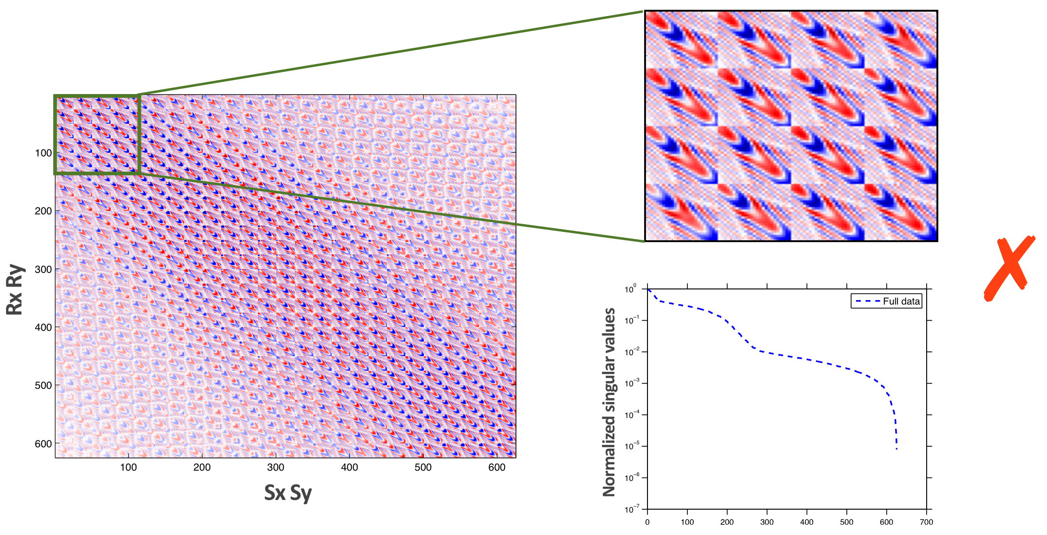
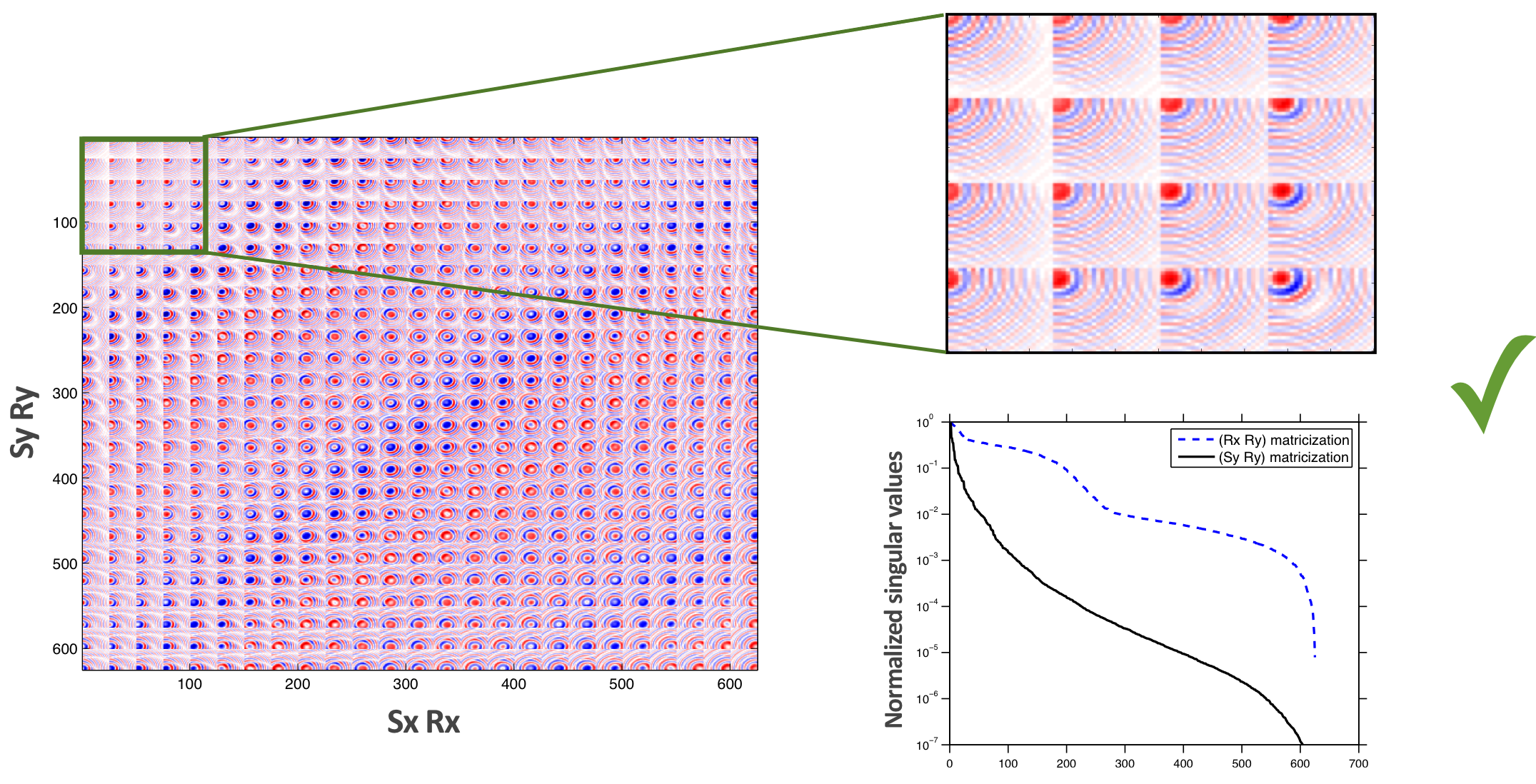
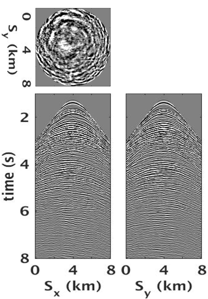
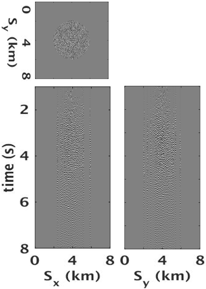
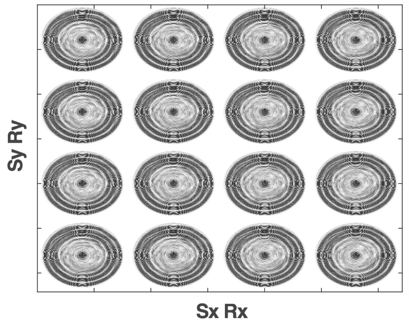
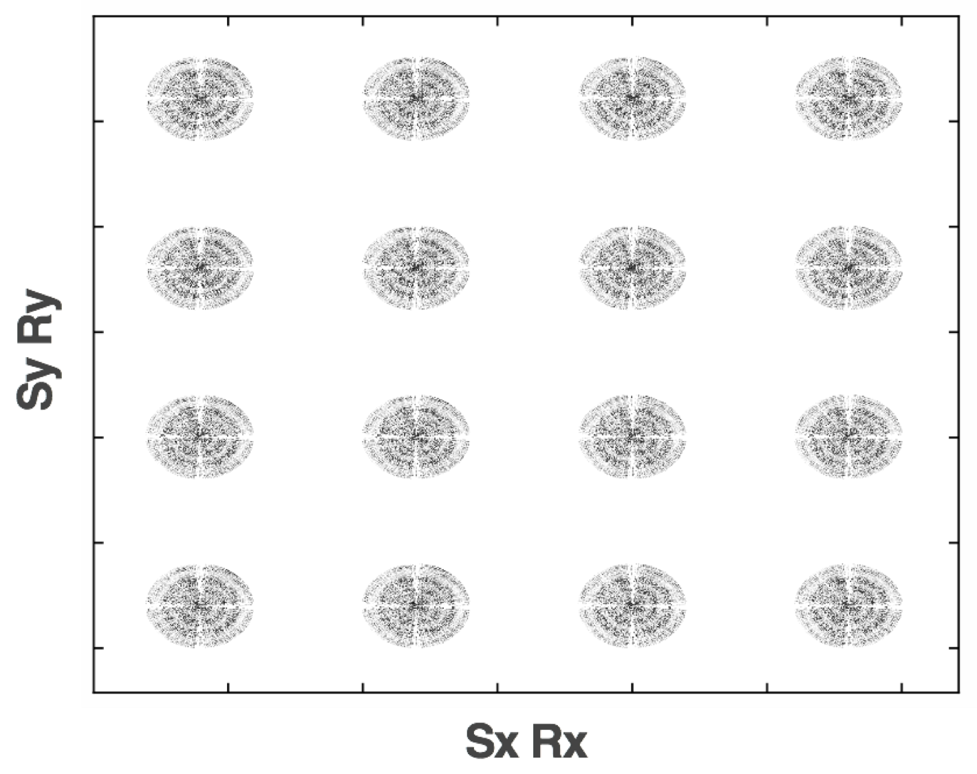
Contrary to exploiting sparsity of vectors, a direct analogue for a matrix is “sparsity” among the singular values, i.e., underlying fully sampled data matrix of interest should exhibit a fast decay of its singular values so seismic data organized as a matrix can be well approximated by a low-rank matrix by ignoring the small singular values. Unfortunately, seismic data does not exhibit a low-rank structure when organized in the canonical matrix representation, where monochromatic shot records appear as columns in the data matrix (Figure 1a). As shown by Kumar et al. (2015b), this problem can for 2D seismic acquisition be overcome by transforming the data to the midpoint-offset domain, which leads to a rapid decay of the singular values. While this approach could be applied to 3D seismic acquisition as well, a simple permutation of matricized seismic data suffices. Here, matricization refers to a process that reshapes a tensor in to a matrix along specific dimensions. In the resulting noncanonical matrix representation (cf. Figures 1a and 1b), the source and receiver coordinates in the \(x-\) and \(y-\)direction are lumped together as opposed to vectorizing monochromatic shot records in the columns as a function of the two source coordinates (Silva and Herrmann, 2013; Kumar et al., 2015a). Because of its simplicity, we use this noncanonical matricization throughout this work.
Break low-rank structure with randomized SLO acquisition
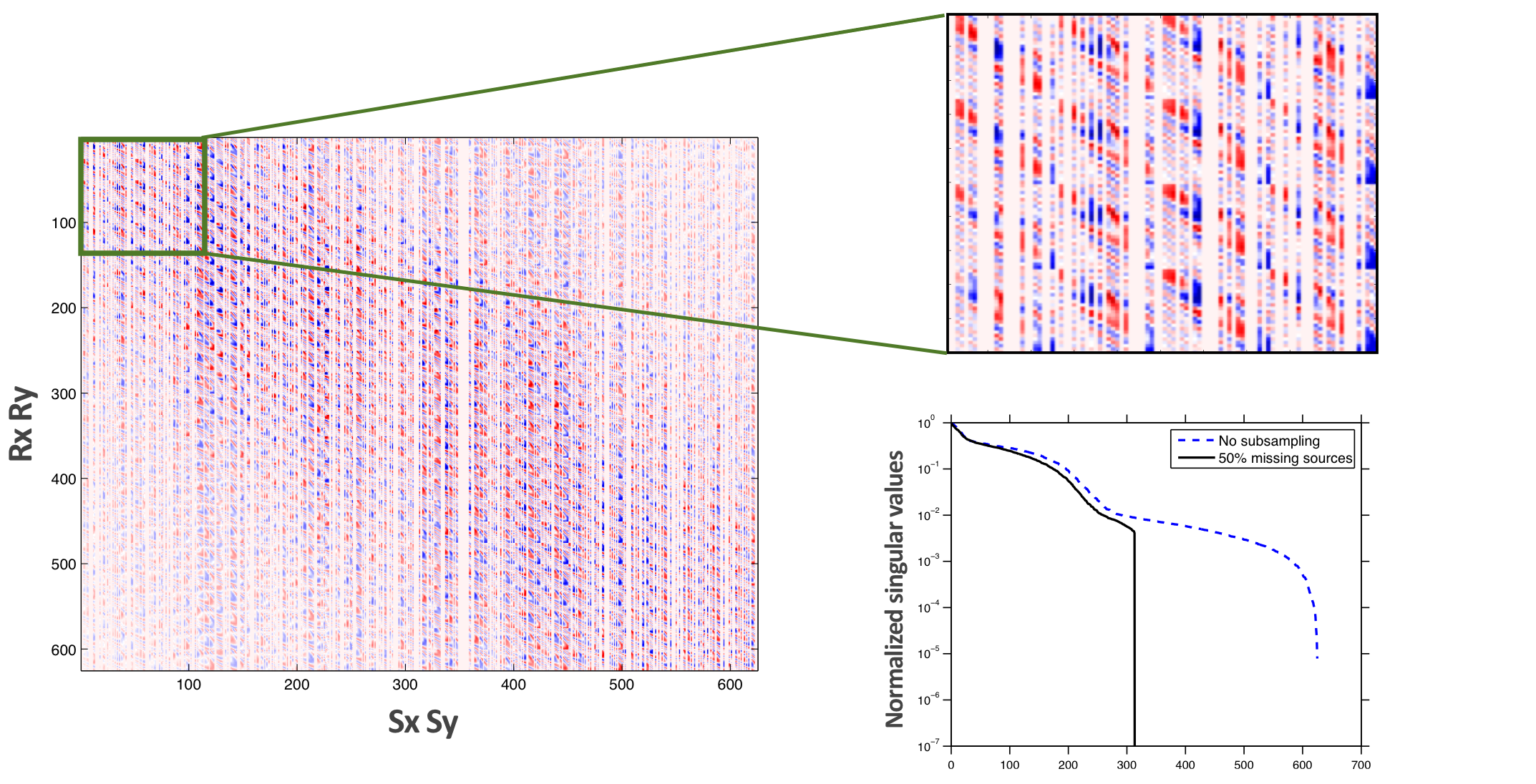
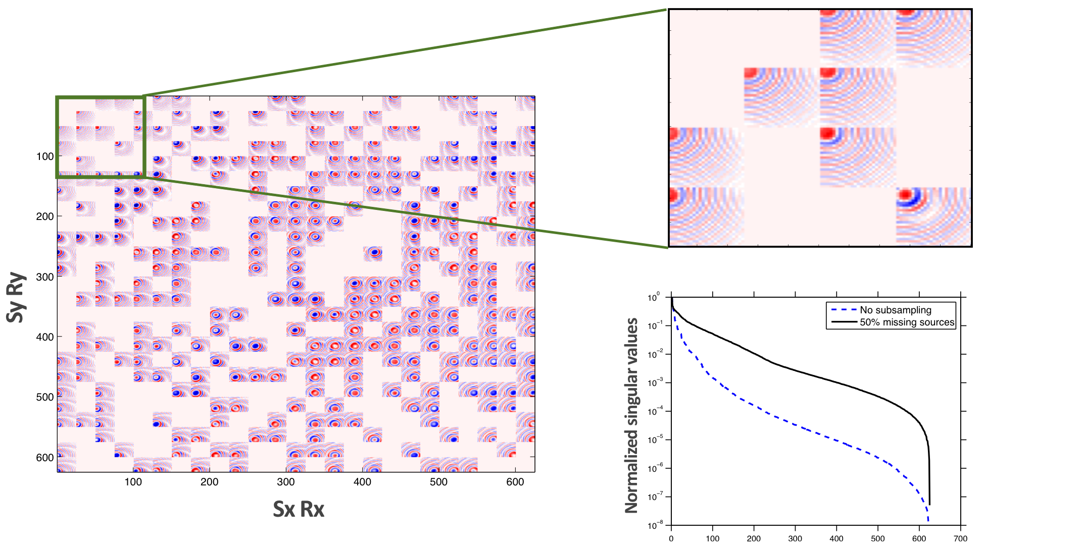
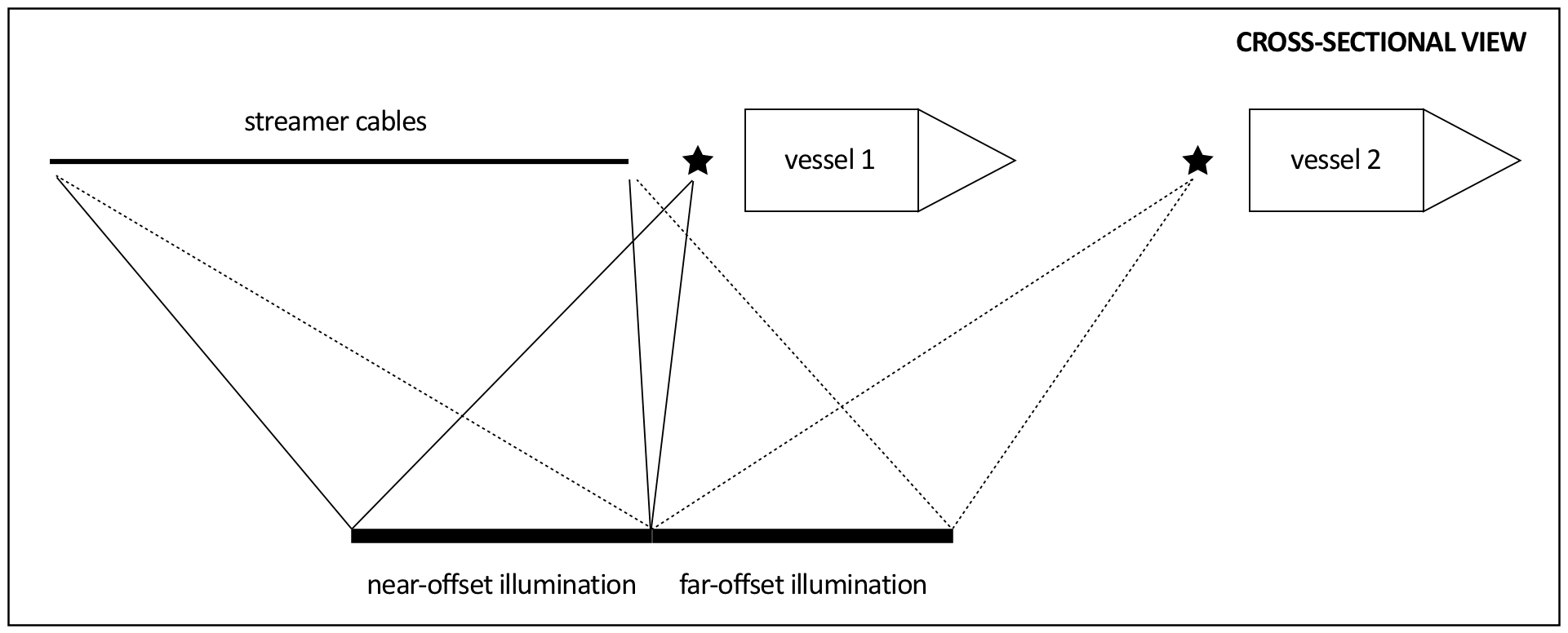
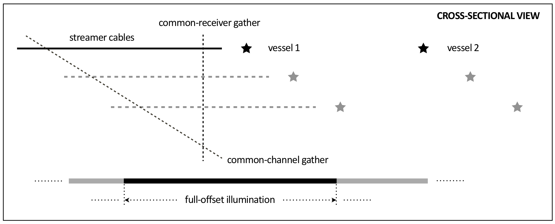
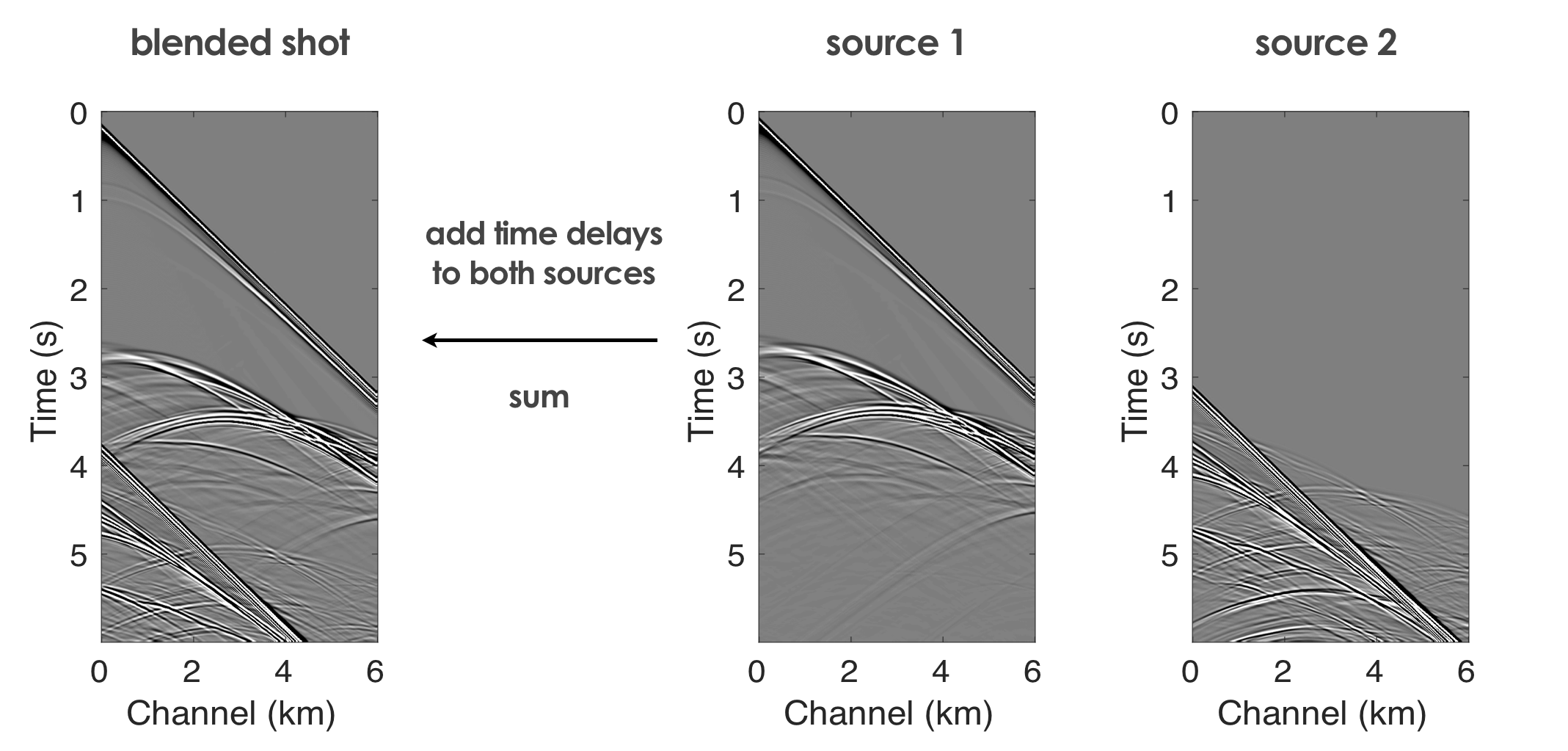
In a nutshell, CS aims to get away with sampling below Nyquist. The way to make this work is to turn coherent subsampling related artifacts, such as aliases, into incoherent noise that does not exhibit structure. For CS with matrices, this corresponds to slowing the decay of the singular values by breaking the low-rank-matrix structure. As we can observe from Figure 1c, randomization of the shot locations in the canonical representation is inadequate because randomly missing shots correspond to randomly missing columns, which lower the rank of the matricized data (cf. the singular-value plots between fully and subsampled data). However, if we consider the behaviour of the singular values for the noncanonical representation the converse is true, i.e., the singular values decay more slowly when sources are missing (Figure 1d). This latter situation is favorable for structure-promoting recovery because we effectively rendered the missing sources into rank inducing “artifacts”. Motivated by this observation for missing traces (Kumar et al., 2015a), and on recent work (Kumar et al., 2015b) that appeared in the literature, we design a 3D towed-streamer simultaneous long-offset (SLO) acquisition, where an extra source vessel (Figure 2) is deployed sailing one spread length ahead of the main seismic vessel (Long et al., 2013), with sources firing at random jittered times within \(1\) or \(2\) second(s) of each other. We have to use this low variability regime in firing times because we are dealing with dynamic acquisition with towed arrays. Compared to highly variable firing times used for static acquisitions with OBC/OBN, the recovery for dynamic blended data is more challenging calling for a reorganization of towed-streamer data in a split-spread geometry, i.e., from the common-channel domain to the common-receiver domain as outlined in Figure 2b. In this common-channel domain, the blended sources are rendered incoherent compared to the summation of the shot gathers themselves (cf. Figures 2c and 2d).
Following Long et al. (2013), we deploy the extra source vessel to double the maximum offset without the need to tow very long streamer cables that can be problematic to deal with in the field. The SLO technique is better than conventional acquisition because it provides a longer coverage in offsets, generally experiences less equipment downtime (doubling the vessel count inherently reduces the streamer length by half), allows for easier maneuvering, and shorter line turns. These practical advantages in conjunction with the observation that random shot-firing times break the structure (Kumar et al., 2015b) make randomized SLO acquisition an excellent candidate to validate our ideas on randomized sampling for time-lapse seismic.

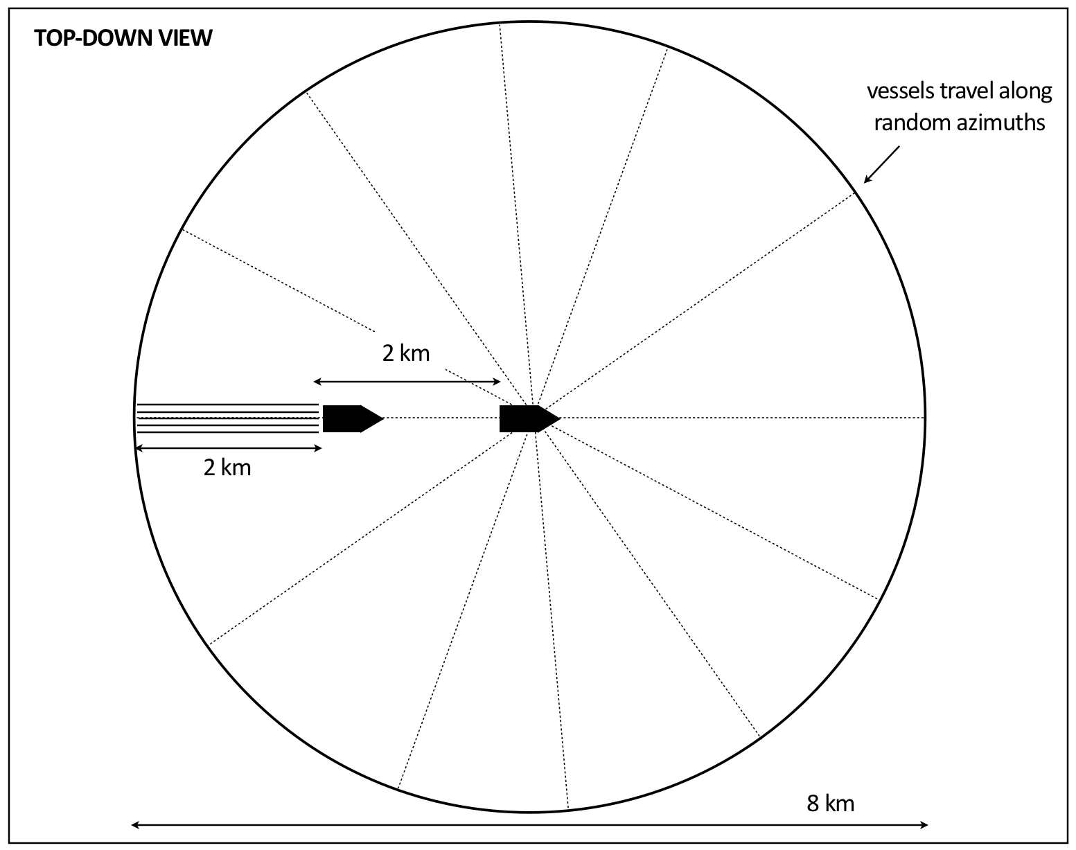
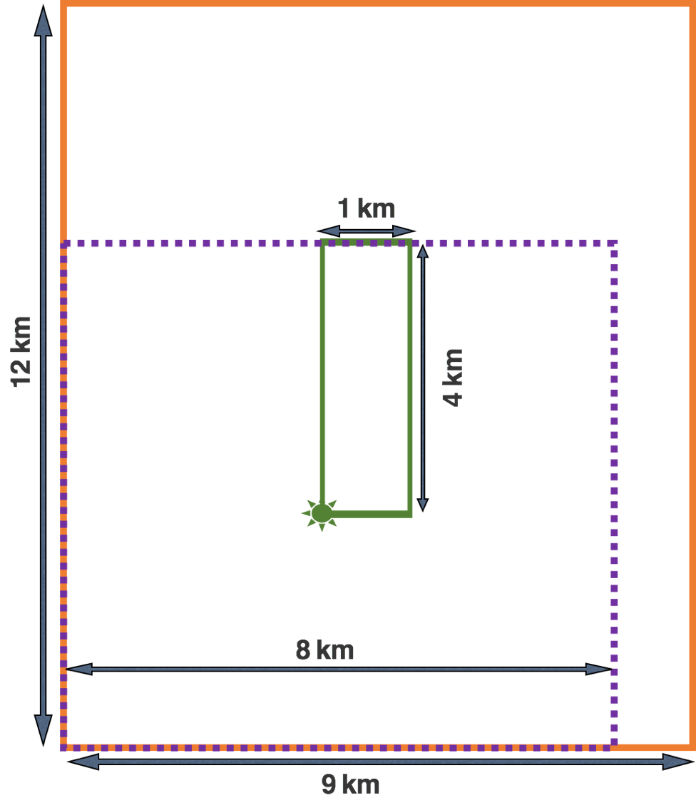
When moving to 3D acquisition, our randomized SLO acquisition design involves, as before, two source vessels with vessel 1 towing 12 streamers. From our and Chuck Mosher’s (Charles et al., 2014) extensive experience in adapting CS to seismic data acquisition, we know that it is beneficial for the later recovery to embrace randomness in the surveys whether this is natural randomness such as cable feathering or randomness by design. For this reason, we opt for our source vessels to travel across the survey area at random azimuths (Figure 3a) with random distance between the sail lines. Recall that we reorganize the towed-streamer data from the common-channel domain to the common-receiver domain (Figure 2b), and therefore Figure 3b shows a source and common-receiver grid for a conventional full-azimuth and offset 3D acquisition. Note that the purple-dash square denotes a “moving-source” grid with respect to the green star representing a common receiver on the fixed green common-receiver grid. The source grid moves as the green star moves along the (fixed) common-receiver grid. Figure 3c shows the randomized SLO acquisition geometry on the underlying conventional full-azimuth and offset 3D acquisition (see the experiment section for SLO acquisition parameter details). We acquire data at 12 random azimuths, which we can reduce further by deploying more source vessels operating at wider azimuths. As a result of the randomization of the sparse sail lines and multi-vessel blended acquisition, the SLO data contains lots of incoherent artifacts (Figure 4b) in contrast to the uneconomical full-azimuth and offset 3D shot record depicted in Figure 4a. For the purpose of recovery by rank minimization, we reorganize the acquired data in the common-receiver domain, where the long-offset information is randomly encoded at the near offsets via the random firing times (cf. Figures 4a and 4b), and therefore is apparently “missing” in Figure 4b. As we will show below, this proposed randomized sampling scheme will allow us to recover \(4\,\times\) maximum-offset source-separated data at a dense \(25\,\mathrm{m}\) source grid (inline and crossline), and a \(25\, \mathrm{m}\) inline and \(100\, \mathrm{m}\) crossline receiver grid from a \(70\%\) source subsampling compared to the conventional long-offset data.

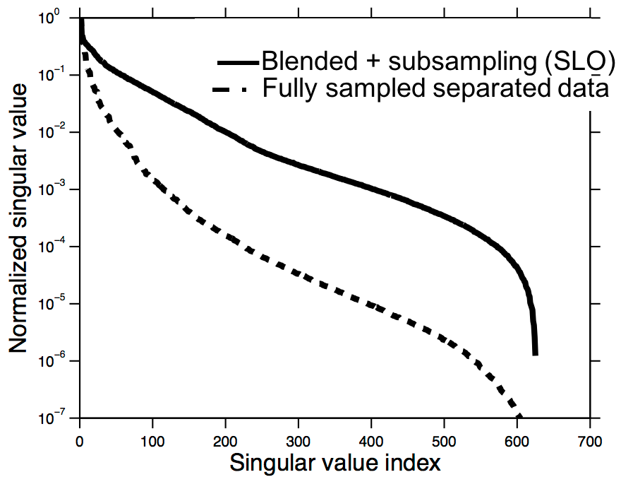
To study the effect of randomization in our 3D SLO acquisition design, we compare the decay of the singular values of conventional dense unfolded (\(4\,\times\) maximum offset) acquisition and our randomized blended acquisition. For this purpose, we included Figures 5a and 5b, which contain a monochromatic frequency slice (at \(10\, \mathrm{Hz}\)) in the noncanonical matricization of the fully sampled data (Figure 5a) and the “offset-compressed” blended data (Figure 5b). As confirmed by Figure 5c, the randomness of the firing times in conjunction with the subsampled SLO acquisition design slows down the decay of the singular values. As a result, we meet the first two main requirements of CS, namely, we have relative fast decay before and slow decay after randomized sparse-azimuth short-offset blended acquisition.
Large-scale factorization-based rank minimization
The third crucial component of CS is the recovery of fully sampled data volumes via structure promotion during which the incoherent subsampling energy is mapped to coherent signal. For this purpose, let us consider the low-rank matrix \({\mathbf{X}}_0\) as an approximation of long-offset densely sampled data organized in the noncanonical \(x_{src}, x_{rec}\) matricization and let \(\mathcal{A}\) be a linear acquisition operator that maps fully sampled data volumes in the frequency domain to data collected in the field with SLO acquisition. Mathematically, the combined action of the sparse-azimuth and blended acquisition can be written as \[ \begin{equation} \begin{aligned} \overbrace{ \begin{bmatrix} {{\mathbf{M}}{\mathbf{T}}_1}{\bf{\mathcal{S}}}^H & {{\mathbf{M}}{\mathbf{T}}_2}{\bf{\mathcal{S}}}^H \end{bmatrix} }^{\mathcal{A}} \overbrace{ \begin{bmatrix} {{\mathbf{X}}}_1 \\ {{\mathbf{X}}}_2 \end{bmatrix} }^{{\mathbf{(X)}}} = {{\mathbf{b}}} , \end{aligned} \label{blendedacq} \end{equation} \] where the observed data is collected in the vector \(\mathbf{b}\) and where \(\mathcal{S}\) is the permutation operator mapping fully sampled seismic data from the vectorized canonical \(x_{src}, x_{rec}\) representation to the noncanonical \(x_{src}, y_{src}\) organization shaped into a matrix. The adjoint, denoted by the superscript \(^H\), does the reverse by applying the permutation from noncanonical to canonical representation, followed by reshaping the monochromatic data into a long vector operated upon by the randomized jitter time delay operators for the two source vessels \({\mathbf{T}}_1\) and \({\mathbf{T}}_2\), followed by subsampling with the restriction matrix \({\mathbf{M}}\) fully determined by the acquisition geometry. As shown in Figure 2c, the two resulting time-shifted and subsampled shot records are according to Equation \(\ref{blendedacq}\) summed into a single blended shot record that models the observed data collected in the vector \(\mathbf{b}\). To simplify the notation, we dropped the frequency dependence and carry out these listed operations in the frequency domain. Once separation and interpolation is finished for each monochromatic data slice, we apply \(\mathcal{S}\) followed by a single inverse Fourier transform along the frequency axis to get the final reconstructed seismic data volume in the time domain.
The task of CS is now to recover an estimate of the fully sampled data represented by the unknown matrix \(\mathbf{X}\) from subsampled data collected in the vector \(\mathbf{b}\). Formally, this recovery can be written as a nuclear-norm minimization problem: \[ \begin{equation} \underset{\mathbf{X}}{\text{minimize}} \quad \|\mathbf{X}\|_* \quad \text{subject to} \quad \|\mathcal{A} ({\mathbf{X}}) - {\mathbf{b}}\|_2 \leq \epsilon, \tag{BPDN$_\epsilon$} \label{BPDNepsilon} \end{equation} \] whose objective it is to minimize the sum of the singular values (denoted by the nuclear norm \(\|\cdot\|_*\) ) while fitting the data to within an error of \(\epsilon\). While theoretically sound, this convex optimization problem does not scale to seismic problems because its solution relies on expensive singular-value decompositions. We overcome this problem by switching to a low-rank representation — i.e., we assume \(\mathbf{X}\approx {{\mathbf{L}}{\mathbf{R}}^H}\) with \(\mathbf{L}\) tall and \(\mathbf{R}^H\) wide. Aside from reducing the memory imprint drastically — the rank (width of \(\mathbf{L}\) and \(\mathbf{R}\)) can be small if the singular values decay fast, this low-rank factorization has the advantage that the optimization (as in Equation \(\ref{BPDNepsilon}\)) can be carried out on the factors alone without forming \(\mathbf{X}\) explicitly. For details on this low-rank factorized recovery, we refer the reader to recent work by Aravkin et al. (2014); Kumar et al. (2015a).
Joint-recovery time-lapse acquisition model
While the above CS framework for SLO acquisition allows for economic marine acquisition because it allows us the “compress” the offset axis in combination with source subsampling, the proposed acquisition scheme has not yet made provisions regarding the collection of time-lapse data involving a baseline survey followed by one or more monitor surveys. Inspired by recent work on low-cost time-lapse seismic with distributed compressive sensing, we adapt our joint-recovery model (JRM) — where we invert for low-rank matrices representing the shared component among the vintages and the differences of the vintages with respect to this component — to the matrix case, i.e., we have \[ \begin{equation} \begin{aligned} \begin{bmatrix} \mathbf{b}_1\\ \mathbf{b}_2\end{bmatrix} &= \begin{bmatrix} {\mathcal{A}_1} & \mathcal{A}_{1} & \mathbf{0} \\ {\mathcal{A}_{2} }& \mathbf{0} & \mathcal{A}_{2} \end{bmatrix}\begin{bmatrix} \mathbf{Z}_0 \\ \mathbf{Z}_1 \\ \mathbf{Z}_2 \end{bmatrix}\quad\text{or} \quad \mathbf{b} = \mathcal{A}(\mathbf{Z}). \end{aligned} \label{eqjrmobs} \end{equation} \] In this JRM, data for the baseline and (in this case single) monitor survey are collected in the vectors \(\mathbf{b}_1\) and \(\mathbf{b}_2\) via the action of the measurements matrices \(\mathcal{A}_{1}\) and \(\mathcal{A}_{2}\) that appear in the above \(2 \times 3\) system that relates the observed data to the low-rank matrix \(\mathbf{Z}_{0}\) for the common component and the low-rank matrices \(\mathbf{Z}_{1}\) and \(\mathbf{Z}_{2}\) for the differences with respect to the common component. We recover low-rank factorizations for the baseline and monitor surveys by solving the optimization problem \(\ref{BPDNepsilon}\), followed by setting \(\mathbf{X}_j = \mathbf{Z}_0 + \mathbf{Z}_j, \ j \in {1,2}\).
The main advantage of this JRM lies in the property that the common component is observed by both surveys \(\mathcal{A}_{1}\) and \(\mathcal{A}_{2}\). So if we chose these surveys sufficiently independent, and this does not take much as we have shown in work published elsewhere, the recovery for the common component and therefore the vintages will improve. This brings us to the main point of this contribution where we conduct a numerical experiment at scale to substantiate our claim that high degrees of repeatability are achievable among time-lapse surveys without insisting on replicating the surveys.
Numerical feasibility study at scale
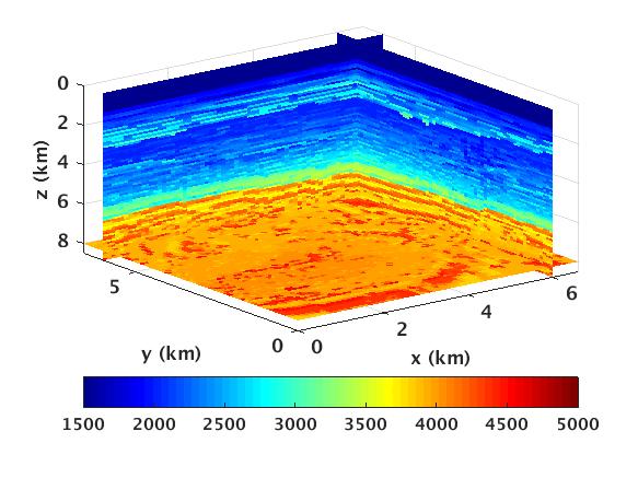
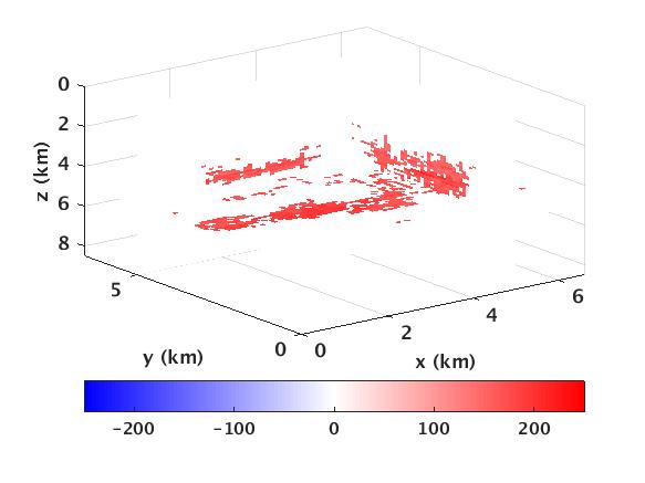
Given the challenge of replicating expensive dense OBC/OBN time-lapse surveys, our aim is to design a 3D randomized towed-streamer time-lapse survey in a realistic field-scale setting. We present a simulation-based feasibility study on two moderately sized 3D synthetic time-lapse vintages generated from the BG COMPASS velocity model (provided by the BG Group). Although the overarching geological structure of the BG COMPASS model is (relatively) simple, it contains realistic well-controlled variability and a complex time-lapse difference related to a gas cloud (Figure 6). The model is \(8\,\mathrm{km}\) deep and \(6.5\,\mathrm{km}\) wide in both lateral directions. In this subset of the BG COMPASS model, the monitor model includes a gas cloud that acts as a proxy for “CO\(_2\)injection”.

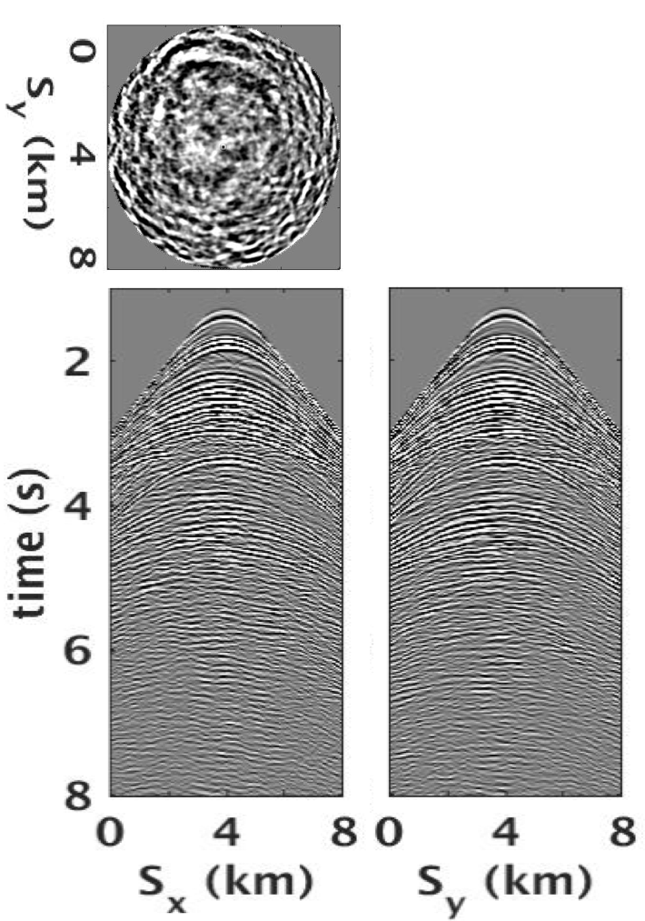
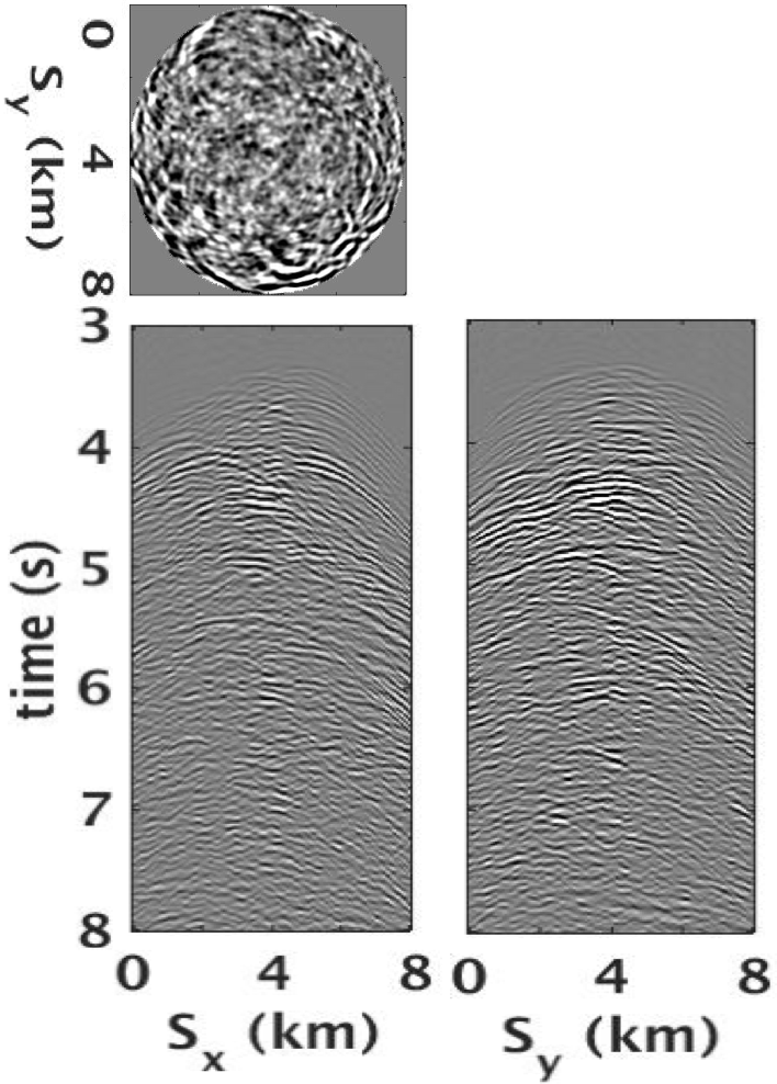
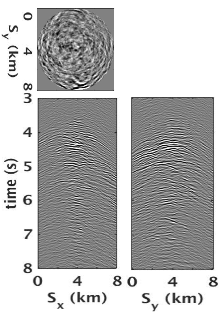
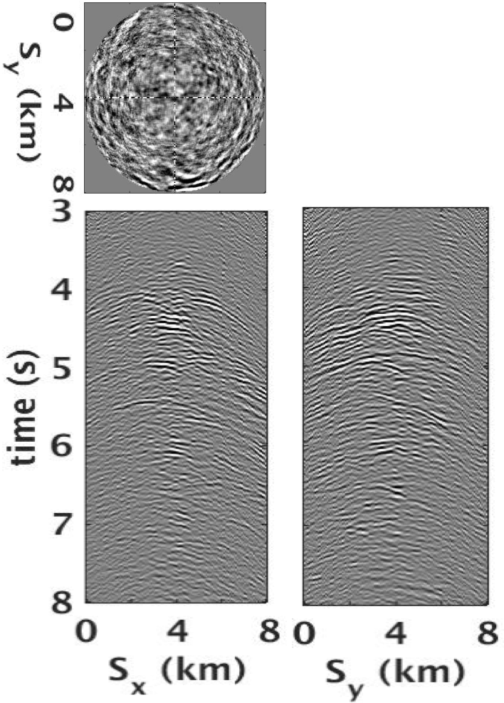
Using an acoustic 3D time-stepping code (Kukreja et al., 2016) and a Ricker wavelet with a central frequency of \(12\,\mathrm{Hz}\), we generate two conventional densely sampled full-azimuth and offset synthetic reference data sets that serve as “ideal” benchmarks for data associated with the baseline and monitor models. Our simulations and subsequent wavefield recovery are carried out over a frequency range of \(5-30\,\mathrm{Hz}\). Each idealized data set contains \(8\, \mathrm{s}\) of data sampled at \(0.004\,\mathrm{s}\) on a \(40 \times 40\) receiver grid and a \(321 \times 321\) source grid. The inline and crossline source sampling, and inline receiver sampling is \(25\,\mathrm{m}\) and the crossline receiver sampling is \(100\,\mathrm{m}\). Figure 7 shows a common-receiver gather from the idealized monitor data and the corresponding time-lapse difference computed by subtracting the idealized baseline and monitor data.
As mentioned earlier, we design a randomized SLO acquisition using two source vessels with vessel 1 towing 12 streamers. Table 1 lists the acquisition parameters used in the acquisition. We collect data at 12 random azimuths, where the vessels move only in the forward direction. Figure 8 shows the randomized SLO time-lapse acquisition geometry on the underlying conventional full-azimuth and offset acquisition grid (cf. Figure 3b). The vessels travel along random azimuths denoted by the blue-dash lines for the baseline survey and the orange-dash lines for the monitor survey. For the SLO data acquisition, we assume that the samples are taken on a discrete grid, i.e., samples lie “exactly” on the grid. The SLO acquisition design results in a \(70\%\) source subsampling for both the baseline and monitor surveys with an unavoidable \(30\%\) overlap between the surveys (measurement matrices \(\mathcal{A}_1\) and \(\mathcal{A}_2\)). We define the term “overlap” as the percentage of on-the-grid shot locations exactly replicated between two (or more) time-lapse surveys.
| No. of streamer vessels | 1 |
| No. of source vessels | 2 |
| No. of source arrays | 4 |
| No. of streamers | 12 |
| Streamer length | 2000 m |
| Group interval | 25 m |
| Shot interval | 25 m |
| Streamer interval | 100 m |
| No. of azimuths acquired | 12 |

Since one of our aims is to attain highly repeatable data without insisting on replicating time-lapse surveys, we compare the performance of our proposed rank-minimization-based source separation and interpolation strategy for different random realizations of the SLO acquisition with \(100\%\) and (the unavoidable) \(30\%\) overlap between the surveys. Given that the observations are subsampled and on the grid, we use the independent recovery model (IRM, Equation \(\ref{BPDNepsilon}\)) and the JRM (Equation \(\ref{eqjrmobs}\)) to recover the vintages and time-lapse difference on a colocated grid corresponding to the conventional full-azimuth and offset 3D acquisition grid. We conduct all experiments using \(20\) nodes with \(5\) parallel MATLAB workers each, where each node has \(20\) CPU cores and \(256\) GB of RAM. We select the maximum number of iterations (\(400\)) and the rank parameter \(k\) (gradually increasing from \(50\) to \(150\) for low to high frequencies) via a cross validation technique on low- and high-frequency slices. The processing time for each frequency slice is about \(9\) hours. Note that we perform source separation and interpolation in the frequency domain, where we invert for each monochromatic slice independently. Once we have all the separated and interpolated monochromatic slices within the spectral band, we perform the inverse temporal-Fourier transform to reconstruct the output time-domain data volume.
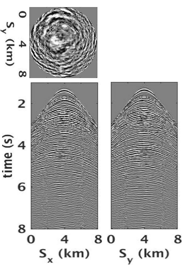
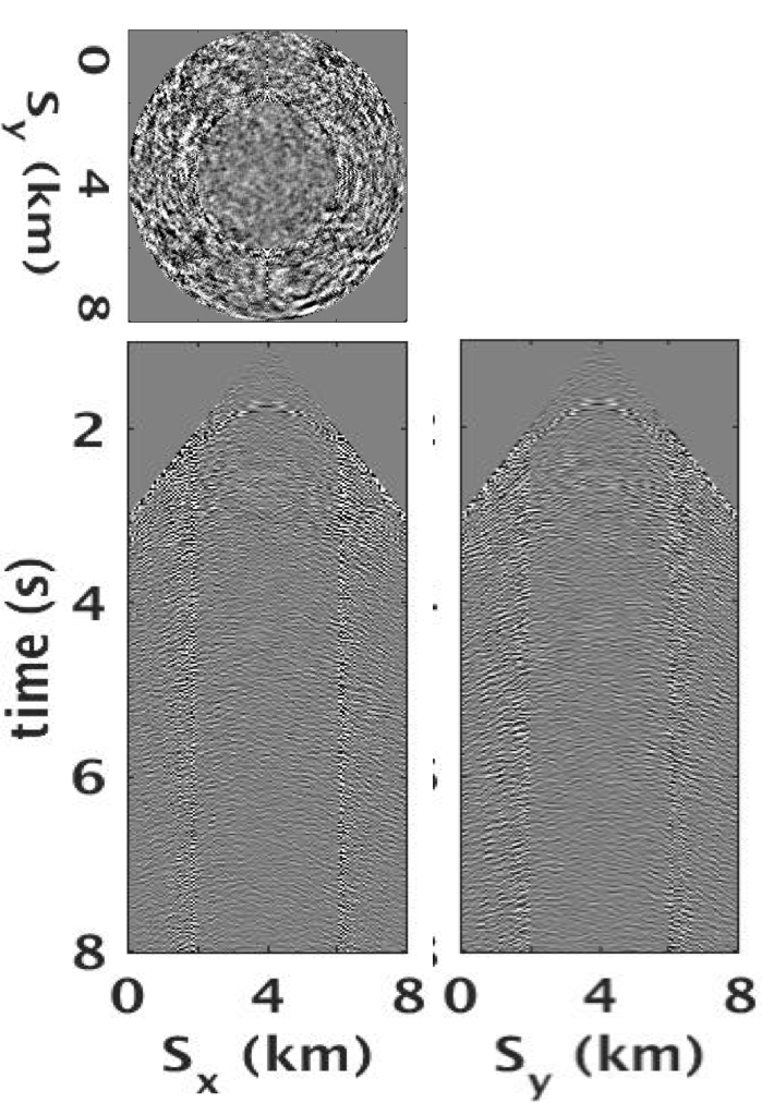
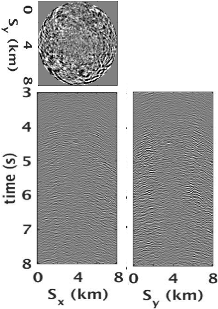
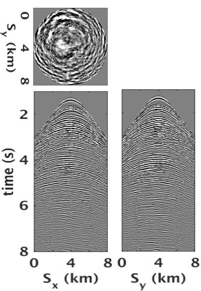
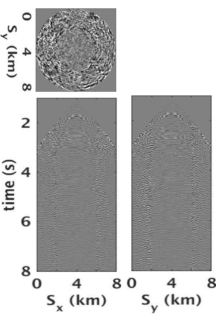
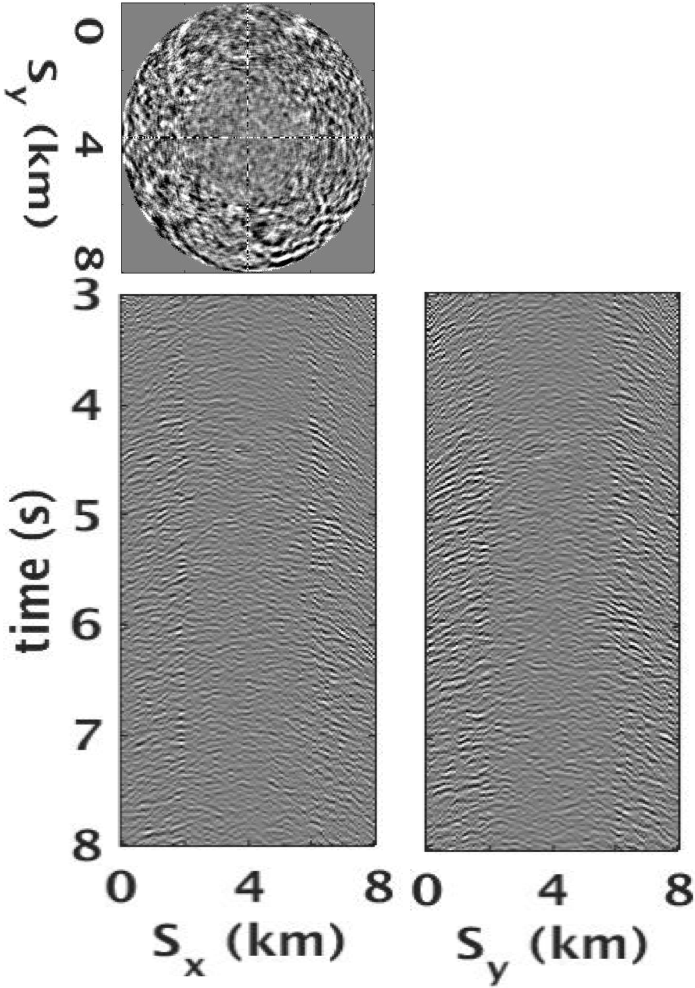
As shown by Oghenekohwo et al. (2017), JRM performs better than IRM because it exploits information shared between the baseline and monitor data, which leads to a formulation where the common component is observed by both surveys. This is also illustrated in Table 2 that shows the signal-to-noise ratio (S/N) of the time-lapse data recoveries. Therefore, we show results for JRM only. Figure 9 shows the JRM-recovered common-receiver gathers and the corresponding residual plots for the baseline data and the time-lapse difference for \(100\%\) overlap between the surveys. The corresponding results for the \(30\%\) overlap are shown in Figure 10. In contrast to \(100\%\) overlap between the surveys, recovery of the vintages (with JRM) is better when the overlap is small. This behaviour is attributed to partial independence of the measurement matrices that contribute additional information via the first column of \(\mathcal{A}\) in Equation \(\ref{eqjrmobs}\), i.e., for time-lapse seismic, independent surveys give additional structural information for the common component leading to improved recovery of the vintages. The converse seems to be true for recovery of the time-lapse difference (although the S/N values are only slightly off (Table 2)) as a result of the increased sparsity of the time-lapse difference itself and apparent cancelations of recovery errors due to the “exactly” replicated geometry. Wason et al. (2017) show that the more realistic and inevitable off-the-grid sampling leads to little variability in recovery of the time-lapse difference for decreasing overlap between the surveys, and hence negates the efforts to replicate. Apart from reasonable reconstruction quality with minimal loss of coherent energy, one of the advantages of using the factorization-based rank-minimization framework is its ability to compress the size of (reconstructed) data volumes significantly, where compression ratio depends upon the rank parameter \(k\). For the conducted experiments, we achieve a compression ratio of \(98.5\%\) for each monochromatic frequency slice of the vintages and time-lapse difference. Table 3 lists the cost savings for our proposed compressive acquisition and recovery strategy.
| Overlap | Baseline | Monitor | 4D signal | |||
|---|---|---|---|---|---|---|
| IRM | JRM | IRM | JRM | IRM | JRM | |
| \(100\%\) | 12.6 | 13.4 | 12.5 | 13.3 | -0.7 | 4.6 |
| \(30\%\) | 12.6 | 15.4 | 10.5 | 15.9 | -7.6 | 3.3 |
| Subsampling ratio | 70% for each vintage |
| Size of each observed vintage | 200 GB |
| Size of each recovered vintage | 800 GB |
| Size of recovered \(\mathbf{L,R}\) factors for each vintage | 12 GB |
| Compression ratio using proposed method | 98.5% |
Discussion and conclusions
By adhering to the principles of compressive sensing, we derive a viable low-cost and low-environmental impact multi-azimuth towed-streamer time-lapse acquisition scheme. Because our formulation exploits structure among time-lapse vintages via low-rank matrix factorizations, we arrive at a scheme that is computationally feasible producing repeatable densely sampled full-azimuth time-lapse vintages from nonreplicated data collected with efficiencies increased by a factor of (approx.) \(3\,\times\). Our findings are consistent with other studies reported in this special issue that indicate that acquisition efficiency can be improved significantly by adapting the principles of CS. In this work, we carry the argument of improving acquisition efficiency with CS a step further by arguing that this new paradigm also provides the appropriate framework for low-cost time-lapse wide-azimuth acquisition with towed arrays and multiple source vessels. We ask these vessels to operate well within their capabilities without insisting on replicating the surveys, which brings down cost making our approach viable in the field.
For simplicity, we limit ourselves to on-the-grid and calibrated surveys, which we do not consider as a limitation because we have shown that our CS-based time-lapse acquisition can be extended to irregular off-the-grid acquisition (Wason et al., 2017) and to situations where the actual and post-plot acquisitions differ by unknown calibration errors. For details on the possible impact of calibration errors, we refer to our companion paper “Highly repeatable time-lapse seismic with distributed Compressive Sensing—mitigating effects of calibration errors” in this special issue. In that contribution, we show that the attainable recovery quality and repeatability of time-lapse vintages and difference deteriorates gracefully as a function of increasing calibration errors. The main contribution of this work is that we confirm, by means of at-scale simulation, that 3D time-lapse full-azimuth multi-vessel towed-streamer acquisition and processing are viable as long as we exploit information shared among the time-lapse vintages, by our joint-recovery model, and within the vintages themselves via low-rank matrix-factorizations (Kumar et al., 2015b). As a result, we arrive at a relatively simple easily parallelizable algorithm that is capable of handling large data volumes without relying on partitioning the data into small volumes. Instead, our permutation into the noncanonical matricization that lumps source/receiver coordinates together, leads to extremely parsimonious representations of the data, which explain the quality and repeatability of the recovered time-lapse vintages from surveys collected with relatively large subsampling ratios without insisting on replication.
In summary, the experience we gain with our numerical feasibility study suggests that we may no longer need to insist on dense replicated source/receiver sampling as in time-lapse surveys with (semi) permanent OBC/OBN. Instead, we demonstrate that high-quality repeatable time-lapse vintages can be acquired with randomized towed-array multi-vessel acquisitions designed according to the principles of CS.
Acknowledgements
We would like to acknowledge Nick Moldoveanu for useful discussions on 3D time-lapse acquisition and Charles Jones (BG Group) for providing the BG COMPASS 3D time-lapse model. This research was carried out as part of the SINBAD project with the support of the member organizations of the SINBAD Consortium. The authors wish to acknowledge the SENAI CIMATEC Supercomputing Center for Industrial Innovation, with support from BG Brasil, Shell, and the Brazilian Authority for Oil, Gas and Biofuels (ANP), for the provision and operation of computational facilities and the commitment to invest in Research & Development.
Abma, R., Ford, A., Rose-Innes, N., Mannaerts-Drew, H., and Kommedal, J., 2013, Continued development of simultaneous source acquisition for ocean bottom surveys: In 75th eAGE conference and exhibition. doi:10.3997/2214-4609.20130081
Aravkin, A. Y., Kumar, R., Mansour, H., Recht, B., and Herrmann, F. J., 2014, Fast methods for denoising matrix completion formulations, with applications to robust seismic data interpolation: SIAM Journal on Scientific Computing, 36, S237–S266. doi:10.1137/130919210
Baron, D., Duarte, M. F., Wakin, M. B., Sarvotham, S., and Baraniuk, R. G., 2009, Distributed compressive sensing: CoRR, abs/0901.3403. Retrieved from http://arxiv.org/abs/0901.3403
Beasley, C. J., 2008, A new look at marine simultaneous sources: The Leading Edge, 27, 914–917. doi:10.1190/1.2954033
Candès, E. J., Romberg, J., and Tao, T., 2006, Stable signal recovery from incomplete and inaccurate measurements: Communications on Pure and Applied Mathematics, 59, 1207–1223. doi:10.1002/cpa.20124
Charles, M., Chengbo, L., Larry, M., Yongchang, J., Frank, J., Robert, O., and Joel, B., 2014, Increasing the efficiency of seismic data acquisition via compressive sensing: The Leading Edge, 33, 386–391. doi:10.1190/tle33040386.1
Donoho, D. L., 2006, Compressed sensing: Information Theory, IEEE Transactions on, 52, 1289–1306.
Kukreja, N., Louboutin, M., Vieira, F., Luporini, F., Lange, M., and Gorman, G., 2016, Devito: Automated fast finite difference computation: ArXiv Preprint ArXiv:1608.08658.
Kumar, R., Silva, C. D., Akalin, O., Aravkin, A. Y., Mansour, H., Recht, B., and Herrmann, F. J., 2015a, Efficient matrix completion for seismic data reconstruction: Geophysics, 80, V97–V114. doi:10.1190/geo2014-0369.1
Kumar, R., Wason, H., and Herrmann, F. J., 2015b, Source separation for simultaneous towed-streamer marine acquisition - a compressed sensing approach: Geophysics, 80, WD73–WD88. doi:10.1190/geo2015-0108.1
Long, A. S., Abendorff, E. von, Purves, M., Norris, J., and Moritz, A., 2013, Simultaneous long offset (SLO) towed streamer seismic acquisition: In 75th eAGE conference & exhibition.
Lumley, D., and Behrens, R., 1998, Practical issues of 4D seismic reservoir monitoring: What an engineer needs to know: SPE Reservoir Evaluation & Engineering, 1, 528–538.
Mansour, H., Wason, H., Lin, T. T., and Herrmann, F. J., 2012, Randomized marine acquisition with compressive sampling matrices: Geophysical Prospecting, 60, 648–662.
Moldoveanu, N., 2010, Random sampling: A new strategy for marine acquisition: In SEG technical program expanded abstracts (pp. 51–55). doi:10.1190/1.3513834
Mosher, C., Li, C., Morley, L., Ji, Y., Janiszewski, F., Olson, R., and Brewer, J., 2014, Increasing the efficiency of seismic data acquisition via compressive sensing: The Leading Edge, 33, 386–391.
Oghenekohwo, F., Wason, H., Esser, E., and Herrmann, F. J., 2017, Low-cost time-lapse seismic with distributed compressive sensing — part 1: Exploiting common information among the vintages: Geophysics, 82, P1–P13. doi:10.1190/geo2016-0076.1
Silva, C. D., and Herrmann, F. J., 2013, Hierarchical Tucker tensor optimization - applications to tensor completion:. SAMPTA.
Wason, H., and Herrmann, F. J., 2013, Time-jittered ocean bottom seismic acquisition: SEG technical program expanded abstracts. doi:10.1190/segam2013-1391.1
Wason, H., Oghenekohwo, F., and Herrmann, F. J., 2017, Low-cost time-lapse seismic with distributed compressive sensing — part 2: Impact on repeatability: Geophysics, 82, P15–P30. doi:10.1190/geo2016-0252.1