![]()
![]()
Abstract
Subsurface-offset gathers play an increasingly important role in seismic imaging. These gathers are used during velocity model building and inversion of rock properties from amplitude variations. While powerful, these gathers come with high computational and storage demands to form and manipulate these high-dimensional objects. This explains why only limited numbers of image gathers are computed over a limited offset range. We avoid these high costs by working with highly compressed low-rank factorizations. These factorizations are obtained via a combination of probings with the double two-way wave equation and randomized singular value decompositions. In turn, the resulting factorizations give us access to all subsurface offsets without having to form the full extended image volumes which are at best quadratic in image size. As a result, we can easily handle situations where conventional horizontal offset gathers are no longer focused. More importantly, the factorization also provides a mechanism to use the invariance relation of extended image volumes for velocity continuation. With this technique, extended image volumes for one background velocity model can be directly mapped to those of another background velocity model. The proposed low-rank factorization inherits this invariance property, so that factorization costs arise only once when examining different imaging scenarios. Because all imaging experiments only involve the factors, they are computationally efficient with costs that scale with the rank of the factorization. Examples using 2D synthetics, including a challenging imaging example with salt, validate the methodology. Instead of brute force explicit cross-correlations between shifted source and receiver wavefields, our approach relies on the underlying linear-algebra structure that enables us to work with these objects without incurring unfeasible demands on computation and storage.
Introduction
The formation of subsurface-offset gathers, such as common-image gathers (CIGs) (Rickett and Sava, 2002; William W Symes, 2008; Stolk et al., 2009; Kalita and Alkhalifah, 2016), angle-domain common-image gathers (ADCIGs) (de Bruin et al., 1990; Kühl and Sacchi, 2003; P. Sava and Fomel, 2003; Mahmoudian and Margrave, 2009; Kroode, 2012; Dafni and Symes, 2016b, 2016a; Kumar et al., 2018), and common-image point gathers (CIPs) (Paul Sava and Vasconcelos, 2011; van Leeuwen and Herrmann, 2012) has become an essential component of modern seismic imaging workflows (Etgen et al., 2009; Dell and Gajewski, 2011). Each type of gathers provides crucial information on the quality of the velocity model and the scattering mechanism. The latter is dependent on the subsurface itself and the acquisition geometry. Contrary to CIGs, CIPs provide information on the complete scattering mechanism because they are functions of the full omni-directional subsurface offset.
Usage of these gathers includes quality control during velocity-model building (Norris et al., 1999), automatic model updates during migration-velocity analysis (W W Symes and Carazzone, 1991; Shen and Symes, 2008), and inferences made on rock properties from amplitude versus offset analysis (de Bruin et al., 1990; Castagna and Backus, 1993; Castagna et al., 1998). All of these usages rely on having access to high-quality subsurface image volumes. While access to fast hardware and memory has made imaging modalities, such as reverse-time migration (RTM)(Baysal et al., 1983; William W Symes, 2007), computationally feasible in 3D (Kukreja et al., 2016; Luporini et al., 2018), the formation of subsurface-offset image volumes remains a major challenge because it involves looping over the sources and multi-dimensional cross-correlations between (shifted) spatio-temporal forward and adjoint wavefields. Aside from the extra computational burden, subsurface-offset or angle image volumes add one or more dimensions to the image space making these volumes more challenging and costly to store and manipulate.
By relying on the wave-equation itself, in combination with a (randomized) probing technique, van Leeuwen et al. (2017) obtain access to full subsurface-offset image volumes via actions of the double two-way wave equation on probing vectors. This double wave-equation is the two-way wave-equation counterpart of Claerbout’s double square-root equation (Jon F. Claerbout, 1970; W W Symes and Carazzone, 1991; Biondi and Symes, 2004; Paul Sava and Vasconcelos, 2011), which is based on the one-way wave equation, limiting its accuracy in media with steeply dipping reflectors. The two-way wave equation remedies this shortcoming.
By choosing probing vectors consisting of a single-point scatterer, van Leeuwen et al. (2017) are able to extract CIPs that are the same size as the original image but now become a function of the omnidirectional subsurface offset. Unlike conventional CIGs, which are generally computed as a function of the horizontal offset alone, CIPs contain offsets in all directions, rendering important advantages in situations with steeply dipping reflectors in which case CIGs no longer focus (see Figure 11 of van Leeuwen et al. (2017)).
While this probing method provides access to an object that can not be formed explicitly—i.e., monochromatic extended image volumes (EIVs) (van Leeuwen et al., 2017) are quadratic in the image size—the cost of this access scales with the number of probing vectors, limiting its use. Despite this shortcoming, the formulation presented by van Leeuwen et al. (2017) provides new insights into migration-velocity analysis and localized amplitude versus offset analysis. These insights include corrections for geologic dips, the derivation of completely novel approaches to velocity continuation (van Leeuwen and Herrmann, 2012; Kumar et al., 2018) that arise from an invariance relation of the double two-way wave equation, and redatuming (Kumar et al., 2019).
Even though the derivation of the double two-way wave-equation results in a fundamentally new approach on how to form and manipulate certain aspects of omnidirectional full-subsurface EIVs, the proposed technique relies on frequency-domain propagators and access to CIPs via probing. This reliance limits its potential application to more realistic imaging scenarios that require time-domain propagators for the wave simulations and call for access to many (geologic-dip) corrected CIGs. To overcome these shortcomings, we propose a low-rank matrix factorization technique, based on the randomized singular value decomposition (rSVD) (Halko et al., 2011) to form EIVs using time-domain wave-equation propagators. To allow low-rank approximations at higher frequencies, where the singular values decay more slowly, we propose a block Krylov method (C. Musco and Musco, 2015), which requires more costly probings but leads to more accurate low-rank factored EIVs.
In addition to achieving a massive compression of EIVs, we will show that low-rank factorizations provide us the access to CIPs and (geologic dip-corrected) CIGs without the need to form EIVs explicitly or to solve additional wave equations—an observation also made by Da Silva et al. (2019), who forms subsurface-offset gathers from a tensor factorization based on the hierarchical Tucker format (Da Silva and Herrmann, 2015). Because EIVs are solutions to the double two-way wave equation, which itself adheres to an invariance relation, they also exhibit this invariance. Remarkably this property is inherited by the proposed low-rank factorization. We will demonstrate that this invariance leads to imaging workflows that incur the relatively high computational costs of the factorization only once. All subsequent imaging costs scale with the rank of the factorization and this includes imaging in different background velocity models. This is clearly a unique property as an image-domain extension of early data-space factorization work by Hu et al. (2009).
The novelty of our contribution is threefold. (1) We construct EIVs via probing (van Leeuwen et al., 2017) with time-domain propagators extending earlier work on low-rank factorization (Kumar et al., 2018) of EIVs with randomized Singular Value Decompositions. (2) To manage the problem of handling and manipulating EIVs at high frequencies, we introduce a power method with Krylov iterations designed to increase the accuracy of low-rank factorizations in situations where the singular values decay slowly. A complexity analysis shows the accuracy of the proposed extension. (3) By extending the invariance relation for factored EIVs, we derive a practical velocity-continuation scheme that reduces both storage and computational costs.
Our contributions are organized as follows. A first section reviews the definition of monochromatic extended image volumes, their relation to the double two-way wave-equation, and a low-rank factorization based on the rSVD. It will be shown how to use this low-rank factorization to migrate and derive CIPs. To accommodate more realistic imaging scenarios, the second half of the first section introduces representations for time-domain EIVs including time-domain probing. Since we are now able to image at high frequencies, a second section is dedicated to presenting and comparing more elaborate probing techniques that involve powers of the double-wave equation. After demonstrating that these methods lead to more accurate factorizations, a third section explains the formation of CIPs and (dip-corrected) CIGs from factors directly without having to form EIVs explicitly. Next, we discuss time-harmonic and time-domain versions of the invariance relationship for EIVs, which allow us to map the EIVs from one background velocity model to another without refactorization. Finally, via carefully selected experiments displayed in a fifth section, the presented factorization approach is validated by comparing true CIPs and CIGs with their approximate counterparts calculated by the proposed approach. We also carry out a realistic imaging scenario involving salt. During that experiment, we demonstrate that imaging scenarios with multiple background velocity models are computationally feasible since we can work on the factors alone. This is possible by virtue of the proposed velocity-continuation approach, derived from the invariance relationship of EIVs (van Leeuwen and Herrmann, 2012; Kumar et al., 2018).
Full subsurface extended image volumes
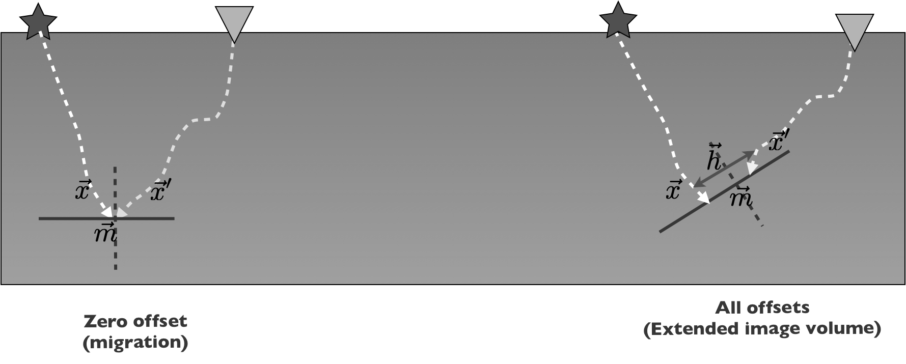
Before discussing our novel approach to factorizing image volumes, we first briefly summarize the formation and probing of image volumes in the frequency and the time domains. The latter allows us to compute image volumes for large-scale problems, including 3D imaging senarios. Compared to regular RTM where the zero-offset imaging condition is applied (Jon F Claerbout, 1985), imaging with extended image volumes (EIVs) (Paul Sava and Fomel, 2006; Paul Sava and Vasconcelos, 2011; van Leeuwen et al., 2017) involves the formation of a “lifted” image volume dependent on two sets of spatial coordinates, one for the source wavefield, with subsurface coordinate \(\vec{x}\) and the other for the receiver wavefield, with subsurface coordinate \(\vec{x}^\prime\). See Figure 1.
Monochromatic extended image volumes
According to van Leeuwen et al. (2017), monochromatic EIVs, with subsurface offsets in all directions, can be formed by a simple outer product. In the Fourier domain, this product can be calculated at the \(i^{\text{th}}\) angular frequency by multiplying the tall matrix \(\mathbf{U}_i\in \mathbb{C}^{N\times n_s}\), containing the discretized monochromatic forward source wavefields collected in its columns for \(n_s\) different sources and \(N=n_x\times n_z\) (with \(n_x,n_z\) number of gridpoints in the \(x-z\) directions) grid points, with the corresponding flat matrix containing the adjoint receiver wavefields \(\mathbf{V}^\ast_i \in \mathbb{C}^{n_s\times N}\). Each monochromatic \(N\times N\) image volume is given by \[ \begin{equation} \mathbf{E}_i = -\omega_i^2\mathbf{V}_i\mathbf{U}_i^*, \label{EIV} \end{equation} \] with \(\omega_i\) the \(i^{\text{th}}\) angular frequency. In this expression, the symbol \({}^*\) represents the complex conjugate transpose of a matrix. This monochromatic image volume represents a discretized version of full monochromatic subsurface image volumes \(E(\vec{x};\vec{x}^\prime)\), where \(\vec{x}=(x,z)\) refers to the spatial subsurface “source” coordinates in 2D and \(\vec{x}^\prime=(x^\prime, z^\prime)\) to a second set of subsurface “receiver” coordinates. For simplicity the frequency dependence is dropped in our notation. From these two sets of coordinates, we define \[ \begin{equation} \vec{m}=\frac{\vec{x}+\vec{x}^\prime}{2}\quad \text{and}\quad \vec{h}=\frac{\vec{x}-\vec{x}^\prime}{2}, \label{eq:offset} \end{equation} \] where \(\vec{m}=(m_x,m_z)\) and \(\vec{h}=(h_x,h_z)\) are the subsurface midpoint and offset coordinates along each spatial coordinate. Semicolons \(;\) are used to separate the coordinate directions so that the discretized image volume can be represented as a matrix.
The above forward and adjoint wavefields satisfy the following forward and adjoint wave equations respectively: \[ \begin{equation} \mathbf{H}_i(\mathbf{m})\mathbf{U}_i = \mathbf{P}_s^\top \mathbf{Q}_i, \label{forward} \end{equation} \] \[ \begin{equation} \mathbf{H}_i^*(\mathbf{m})\mathbf{V}_i = \mathbf{P}_r^\top \mathbf{D}_i, \label{adjoint} \end{equation} \] where \(\mathbf{H}_i(\mathbf{m}),\, i=1\cdots n_f\), \(nf\) is the number of frequencies, which represents the discretized Helmholtz operator at the \(i^{\text{th}}\) frequency. The Helmholtz operator itself is parameterized by the discretized squared slowness collected in the vector \(\mathbf{m}\in \mathbb{R}^N\). The \(n_s \times n_s\) matrix \(\mathbf{Q}_i\) denotes the source matrix, where \(n_s\) is the number of sources. The observed data are collected in monochromatic \(n_r \times n_s\) complex-valued data matrices \(\mathbf{D}_i,\,i=1\cdots n_f\), where each column represents a single monochromatic source experiment with \(n_r\) receivers. Matrices \(\mathbf{P}_s\) and \(\mathbf{P}_r\) are projection operators that restrict the full wavefields to the source and receiver positions, respectively. The symbol \({}^\top\) denotes the matrix transpose. By substituting equations \(\ref{forward}\) and \(\ref{adjoint}\) into equation \(\ref{EIV}\), the EIVs \(\mathbf{E}_i,\,i=1\cdots n_f\) can be expressed as a function of \(\mathbf{Q}_i\) and \(\mathbf{D}_i\) as follows: \[ \begin{equation} \begin{aligned} \mathbf{E}_i &= -\omega_i^2 \mathbf{H}_i^{-*}\mathbf{P}_r^\top \mathbf{D}_i \mathbf{Q}_i^* \mathbf{P}_s \mathbf{H}_i^{-*}\\ &= \mathbf{H}_i^{-*}\mathbf{P}_r^\top \dot{\mathbf{D}}_i \dot{\mathbf{Q}}_i^* \mathbf{P}_s \mathbf{H}_i^{-*}. \end{aligned} \label{fullEIV} \end{equation} \] Here the symbol \(^{-*}\) stands for the conjugate inverse, which is the conjugate transpose of the matrix inverse denoted by the symbol \(^{-1}\). To simplify our notation, we introduce the \(\dot{}\) symbol to denote the inclusion of the \(j\omega_i\) factor into the definition of the source and data matrices. With this notation, equation \(\ref{fullEIV}\) corresponds to the solution of the double two-way wave-equation (van Leeuwen et al., 2017), which is given by \[ \begin{equation} \mathbf{H}_i^{*}\mathbf{E}_i \mathbf{H}_i^{*}= \mathbf{P}_r^\top \dot{\mathbf{D}}_i \dot{\mathbf{Q}}_i^* \mathbf{P}_s. \label{eq:two-way} \end{equation} \] During migration, EIVs are computed using a background velocity model that defines the squared slowness in the above discretized Helmholtz operators. Assuming this background velocity model is known, we are interested in finding ways to form and manipulate image volumes in realistic imaging scenarios. Because \(N\) easily grows too large, it becomes unfeasible to form, store, or even manipulate EIVs in explicit form. This issue is addressed by exploiting the reported low-rank properties of EIVs (van Leeuwen et al., 2017; Kumar et al., 2018; Yang et al., 2019). Without loss of generality, we will work exclusively on 2D imaging problems that can feasibly be extended to 3D. Focus will be on accuracy and develop techniques that cast EIVs into factored form, which allows for computationally feasible manipulation and extraction of useful gathers for migration velocity analysis, amplitude-versus-offset analyses, and redatuming (van Leeuwen et al., 2017; Kumar et al., 2019).
As in earlier work by van Leeuwen et al. (2017), our approach relies on probing EIVs, that is, computing the action of EIVs on certain probing vectors. Aside from giving us access to (CIPs)—i.e. full omnidirectional subsurface-offset gathers, probings provide information required for factoring EIVs using rSVDs (Halko et al., 2011). To enable scale up, we extend earlier work by using wave propagators based on time stepping, in combination with a more sophisticated randomized probing methodology. Before introducing probing with time stepping, probing of monochromatic EIVs is briefly reviewed first. It is shown how this probing technique leads to an alternative formation of subsurface zero-offset RTM.
Low-rank factorization of time-harmonic EIVs
To form \(N\times N\) , with \(N\) the subsurface grid points, EIVs in a computationally feasible manner, the action of these volumes is computed on a limited number, \(n_p\), of monochromatic probing vectors collected in the tall matrix \(\mathbf{W}_i \in \mathbb{C}^{N\times n_p}\) with \(n_p< n_s\ll N\). Following van Leeuwen et al. (2017), the probing entails \[ \begin{equation} \mathbf{Y}_i = \mathbf{E}_i\mathbf{W}_i = \mathbf{H}_i^{-*}\mathbf{P}_r^\top \dot{\mathbf{D}}_i \dot{\mathbf{Q}}_i^* \mathbf{P}_s \mathbf{H}_i^{-*} \mathbf{W}_i, \label{EIVprob} \end{equation} \] which involves \(2n_p\) wave-equation solves. There are several different choices possible for \(\mathbf{W}_i\). For now1, we choose the entries of \(\mathbf{W}_i\) to be drawn from zero-centered Gaussian noise with unit standard deviation to reap the range of \(\mathbf{E}_i\) (Kumar et al., 2018).
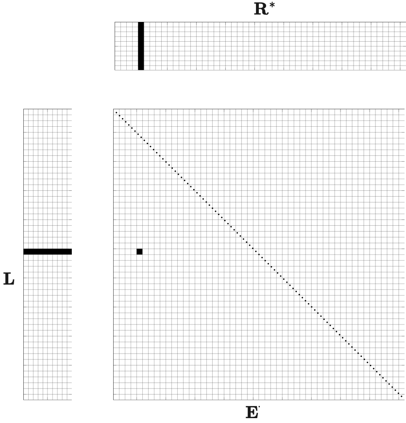
In situations where EIVs can be approximated accurately by a low-rank matrix, the result of the probing \(\mathbf{Y}_i\) accurately captures information on the range of \(\mathbf{E}_i\) as long as \(n_p\) is slightly larger than the rank \(k\) (Halko et al., 2011). Information reaped via the above probing, allows us to approximate EIVs via the following low-rank factorization: \[ \begin{equation} \mathbf{E}_i\approx \mathbf{L}_i\mathbf{R}_i^\ast, \label{LR} \end{equation} \] where the factors \(\mathbf{L}_i\) and \(\mathbf{R}_i \in \mathbf{C}^{N\times n_p}\) are computed with the rSVD (Halko et al., 2011) as described in Algorithm 5, included in Appendix A. This algorithm takes the above probing as input and produces \(\{\mathbf{L}, \mathbf{R}\}\) factors derived from an SVD on a flat system of equations (see Algorithm 5). Compared to a regular SVD, which takes \(\mathcal{O}(N^3)\) to factorize an \(N\times N\) matrix, the rSVD needs only \(\mathcal{O}(2 N n_p^2)\) operations. However, the rSVD requires the action of \(\mathbf{E}\) and \(\mathbf{E}^\ast\) on vectors at a cost of \(2n_p\) wave-equation solves each.
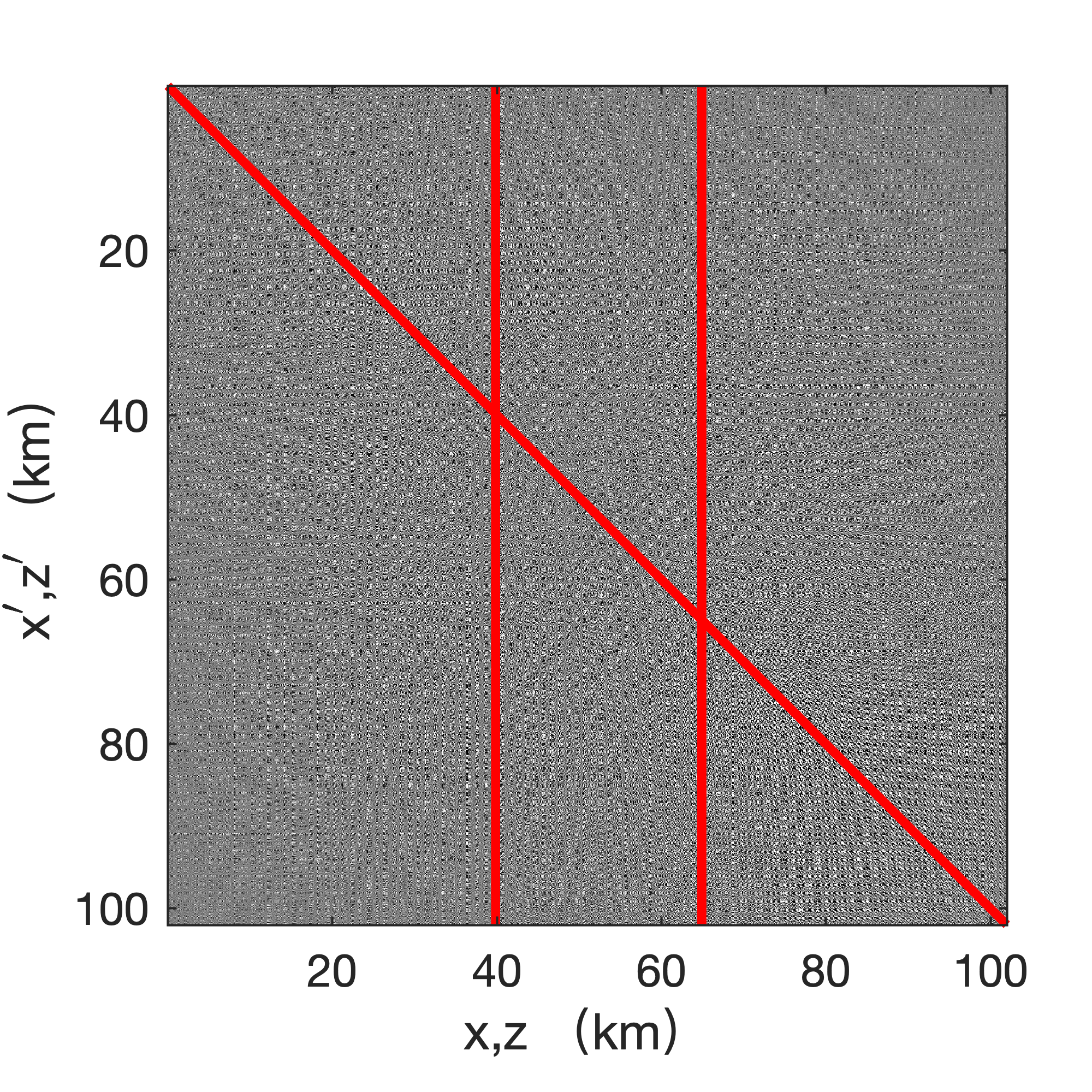
To illustrate the concept of factorizing EIVs with rSVDs, we consider a small EIV, with \((N=100\times 100)\), computed from a subset of the 2D synthetic Marmousi model (Versteeg, 1994) discretized at frequencies ranging between \(5\,\mathrm{Hz}\) and \(50\,\mathrm{Hz}\) with a step of \(0.5\,\mathrm{Hz}\). Given these rSVDs, the behavior of the singular values and the frequency dependence of its low-rank factored approximation is studied. In addition to allowing the formation of full subsurface-offset image gathers, the low-rank factorization also privides access to zero subsurface-offset migrated images via \[ \begin{equation} \delta\hat{\mathbf{m}}=\sum_{i=1}^{n_f}\operatorname{diag}(\mathbf{E}_i)\approx\sum_{i=1}^{n_f}(\mathbf{L}_i\odot\mathbf{\bar{R}}_i)\mathbf{1}. \label{eq:RTM-diag} \end{equation} \] In this expression, \(\operatorname{diag}(\,)\) extracts, for each frequency, the diagonal from the EIVs. The symbol \(\odot\) corresponds to elementwise multiplication also known as the Hadamard product. The symbol \(\bar{\,}\) represents complex conjugation and \(\mathbf{1}\) corresponds to a column vector with \(n_p\) \(1\)’s. In the first part of equation \(\ref{eq:RTM-diag}\), the sum over frequencies corresponds to the zero time-lag imaging condition (Jon F Claerbout, 1985; Berkhout, 1986), while extraction of the diagonal corresponds to imposing the zero subsurface-offset imaging condition. Then, the second part of equation \(\ref{eq:RTM-diag}\) reminds that the diagonal extraction is equivalent to taking the Hadamard product of the factors for each frequency, followed by summing over the columns.
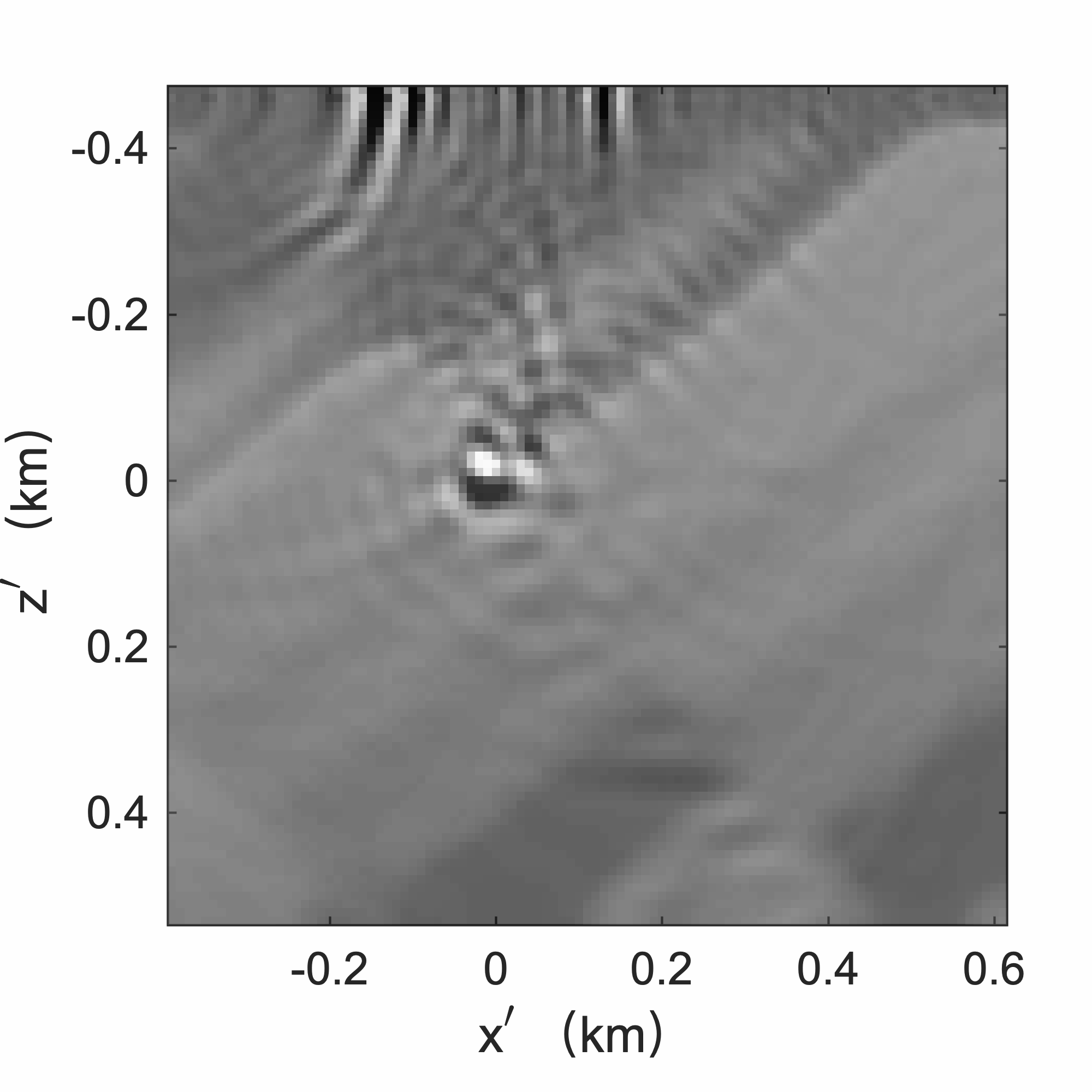
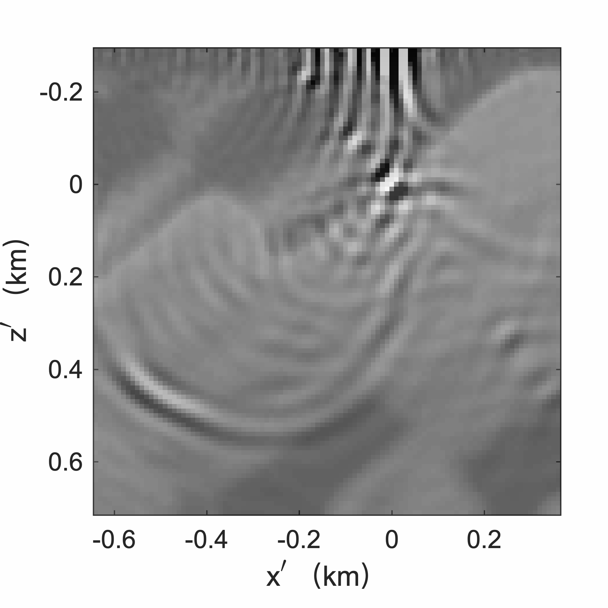
Results of this procedure are summarized in Figure 2, where we show how to extract a zero-subsurface offset migrated image (Figure 2b) from the diagonal of the EIV plotted in Figure 2a. In addition to including information on the migrated image, EIVs also contain CIPs. The latter can be formed by extracting columns from the EIVs, followed by summing the real part over frequency. As with migration (cf. equation \(\ref{eq:RTM-diag}\)), this information is accessible from the low-rank factored form given in equation \(\ref{LR}\). As long as we increase the rank from \(n_p=10\) to \(40\) for the higher frequencies, the low-rank approximation in equation \(\ref{eq:RTM-diag}\) yields images and CIPs close to those obtained via regular RTM, which require a loop over all \(n_s\) sources. Compared to conventional CIGs, CIPs contain full-subsurface offsets in all directions (van Leeuwen et al., 2017). As a result, they provide information on the directivity pattern and geologic dip of the various reflectors, as one can see from the overlays in Figures 2c and 2d.

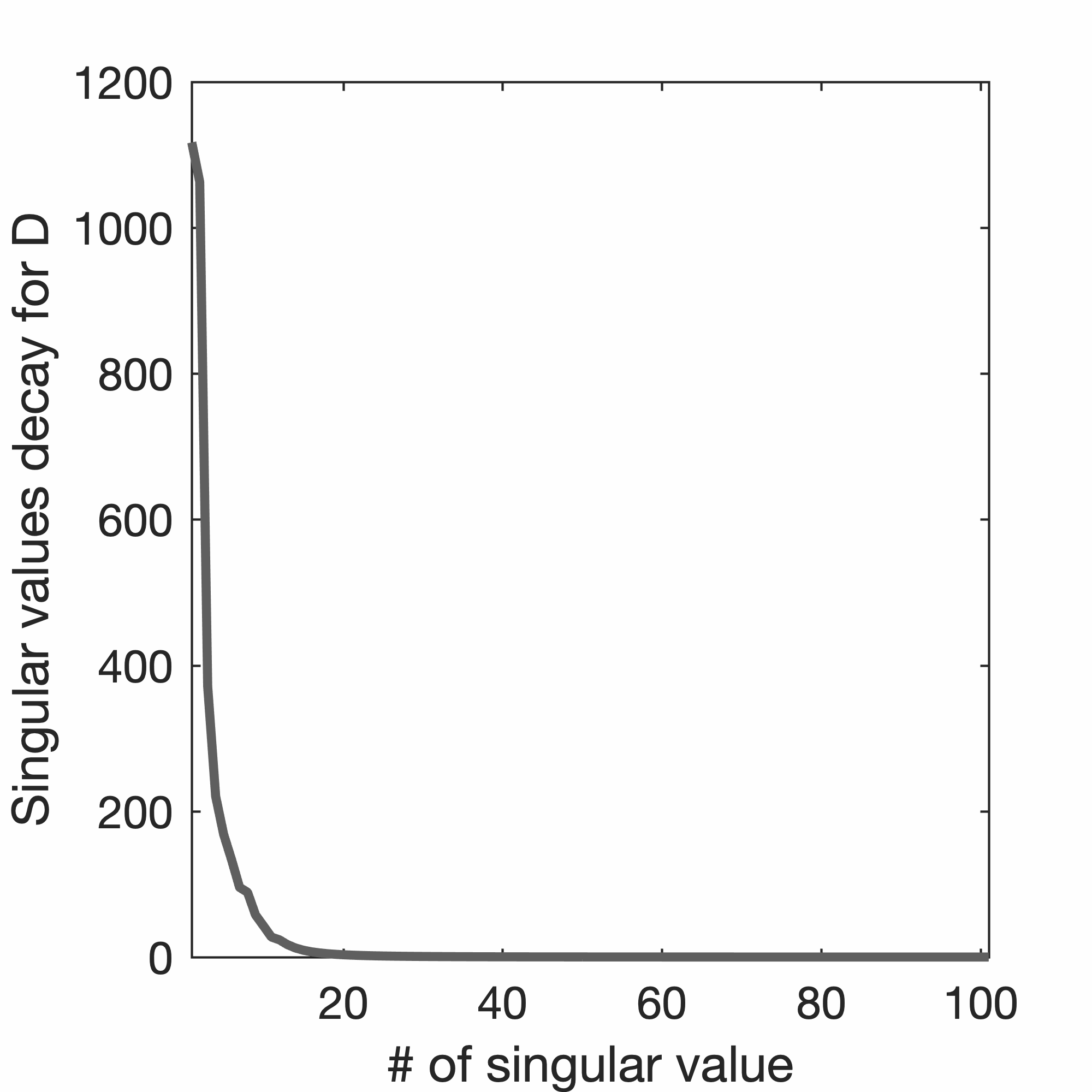
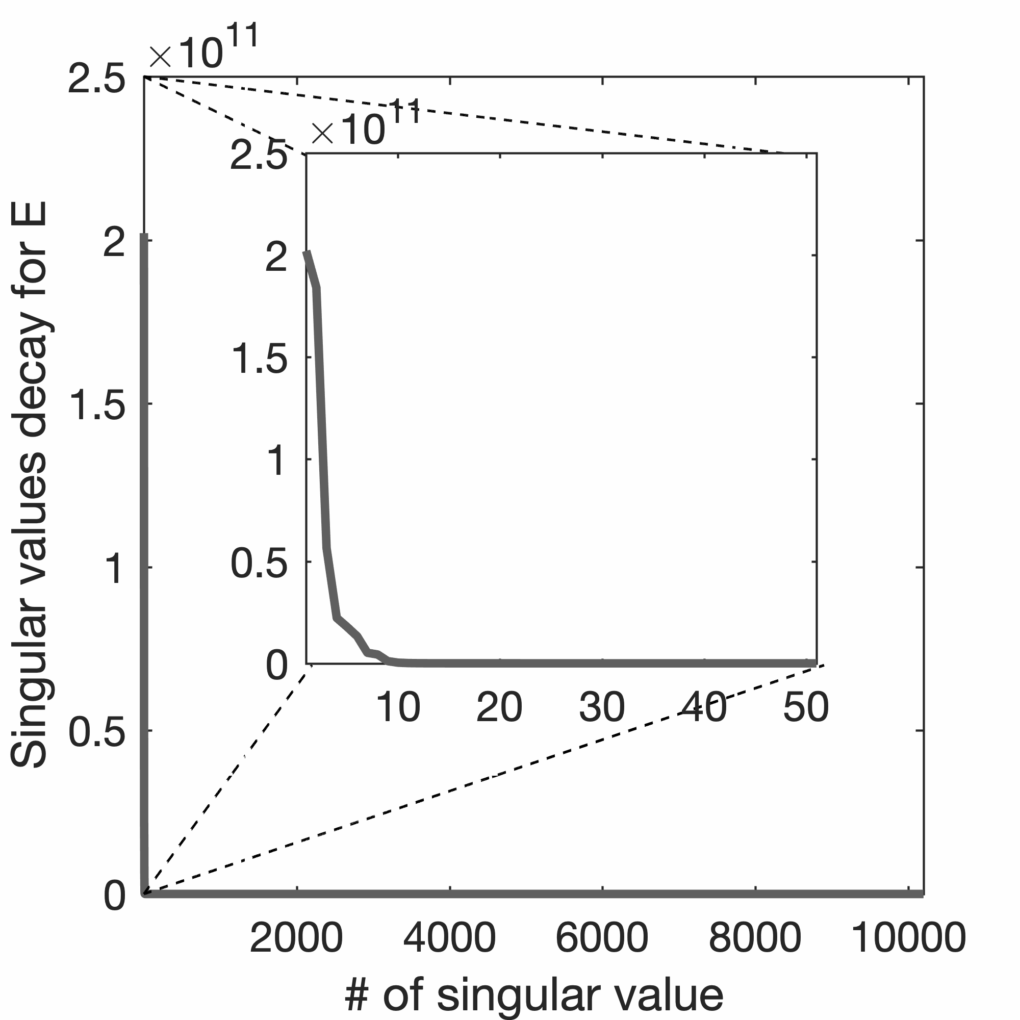
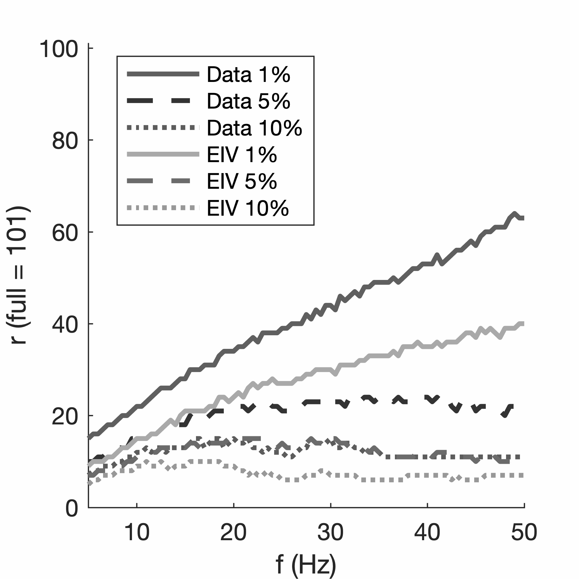
The results in Figure 2 are obtained by making use of the relative faster decay for the singular values of the EIVs compared to the decay for the singular values of the data matrix, as illustrated in Figures 3 and 4. This suggests that the real aim is to factorize EIVs rather than the data itself as proposed by Hu et al. (2009). However, this fast decay for the singular values slows down as the frequency increases. This effect is illustrated in Figure 4, which shows the rank to choose for each frequency in order to capture the singular values to within a \(1\%\), \(5\%\) or \(10\%\) of the largest singular value. Since the decay of the singular value decreases with frequency, the minimal rank to select increases with frequency. Fortunately, this effect does not appear to be as strong in the EIVs as it is in the data, and this explains why \(n_p=9 - 40\) is sufficient in the example included in Figure 2.
While the above approach allows for the formation and manipulation of EIVs in low-rank factored form without explicitly forming the EIV matrix, scaling this approach to more realistic imaging settings still entails several challenges, including larger 2D or even 3D imaging problems and higher frequencies. Both of these call for computationally more efficient wave propagators and randomized SVDs able to factor matrices that can not be approximated accurately by low-rank factorizations using standard randomized probing techniques. Before demonstrating our approach on more realistic examples, let us first discuss how to probe with time-stepping propagators and how to handle the factorization of high-frequency EIVs.
Time-domain EIVs
To substitute time-harmonic wave-equation solvers in equation \(\ref{fullEIV}\) with scalable time-stepping based on finite-difference operators, we introduce the discrete temporal forward, \(\mathsf{U}\), and adjoint wavefields \(\mathsf{V}\) as solutions of \[ \begin{equation} \mathcal{A}(\mathbf{m}) [\mathsf{U}]= \mathcal{P}_s^\top [ \mathsf{Q}] \label{forward_time} \end{equation} \] and \[ \begin{equation} \mathcal{A}^\top(\mathbf{m}) [ \mathsf{V}] = \mathcal{P}_r^\top [ \mathsf{D}]. \label{adjoint_time} \end{equation} \] In these expressions, the symbols \(\mathsf{U} \in \mathbb{R}^{n_t \times N \times n_s}\) and \(\mathsf{V} \in \mathbb{R}^{n_t\times N \times n_r}\) are tensors representing the forward and adjoint wavefields, respectively, where \(n_t\) is the number of time samples. The linear operator \(\mathcal{A}\) denotes the discretized wave-equation, which is solved via time stepping using Devito2. Similarly, the adjoint wavefield is solved for via backward time-stepping with the adjoint \(\mathcal{A}^\top\). The square brackets \([\,]\) are used to indicate the application of linear time-domain operators to wavefields represented as tensors. The source terms for these wave equations are given by impulsive sources and data, collected in the tensors \(\mathsf{Q}\) and \(\mathsf{D}\). These terms are injected into the computational grid via transposes of linear operators \(\mathcal{P}_s\) and \(\mathcal{P}_r\).
With these definitions for the time-domain wavefields, we can write the time-domain EIV as follows: \[ \begin{equation} \begin{aligned} \mathsf{E}&= &\dot{\mathsf{V}}\ast_t\dot{\mathsf{U}}^\top\\ &=& \mathcal{F}^\top[\dot{\mathbf{V}} \cdot \dot{\mathbf{U}}^\ast].\\ \end{aligned} \label{fullEIV_time_conv} \end{equation} \] As before, we absorb time differentiation denoted by the dot symbol \(\dot{}\). The symbol \(\ast_t\) stands for multi-dimensional temporal convolution3 between the two time-differentiated wavefields \(\dot{\mathsf{V}}\) and \(\dot{\mathsf{U}}^\top\). The convolutions are implemented via matrix-matrix multiplications of the monochromatic frequency slices \(\dot{\mathbf{V}_i}\) and \(\dot{\mathbf{U}^\ast_i}\), \(i=1\cdots n_f\). In the second part of equation \(\ref{fullEIV_time_conv}\), the \(\cdot\) operator is introduced as a shorthand for carrying out these multi-dimensional convolutions for each frequency. Finally, we obtain the time-domain EIV by applying the inverse Fourier transform \(\mathcal{F}^\top\) along the time coordinate.
To set the stage for the probing of EIVs formed with the above time-domain propagators, equation \(\ref{fullEIV_time_conv}\) can be rewritten as \[ \begin{equation} \begin{aligned} \mathbf{E} &= \overbrace{\mathcal{F} \circ \mathcal{A}^{-\top} \circ \mathcal{P}_r^\top [ \dot{\mathsf{D}}]}^{\dot{\mathbf{V}}} \cdot \overbrace{(\mathcal{F} \circ \mathcal{A}^{-1} \circ \mathcal{P}_s^\top [ \dot{\mathsf{Q}}])^\ast}^{\dot{\mathbf{U}}^\ast} \\ &= \mathcal{F} \circ \mathcal{A}^{-\top} \circ \mathcal{P}_r^\top \circ \mathcal{F}^\top [ \dot{\mathbf{D}} \cdot \dot{\mathbf{Q}}^* \cdot ( \mathcal{F}\circ \mathcal{P}_s \circ \mathcal{A}^{-\top} [\mathsf{I}] )]. \end{aligned} \label{fullEIV_time} \end{equation} \] In this expression, the symbol \(\circ\) refers to the composition operator of time-domain operators. The symbol \(\mathbf{E}\) is used as a shorthand for \(\{\mathbf{E}_i\}_{i=1}^{n_f}\). Clearly, the above expressions represent the double two-way wave equation (cf. equation \(\ref{eq:two-way}\)) as proposed by van Leeuwen et al. (2017) but they are now based on wave propagators computed via time-stepping. The temporal convolutions are carried out by the complex-valued matrix-matrix products in the temporal Fourier domain. The tensor \(\mathsf{I}\) contains a set of monochromatic identity matrices \(\mathbf{I}_i \in \mathbb{C}^{N \times N}\), where \(i=1\cdots n_f\).
Time-domain probing
While equations \(\ref{fullEIV_time_conv}\) and \(\ref{fullEIV_time}\) in principle allow us to form EIVs in the time or Fourier domain using time-domain propagators, these expressions do not lend readily themselves to probing. For instance, time-stepping propagators impose additional conditions on the wavefields they propagate. This means that the source wavefield has to be bandwidth-limited in the time domain to ensure stability of finite-difference schemes. To make sure that this requirement is met, a single temporal source signature is defined for all sources. In addition, we the sources are modelled by Dirac distributions in space—i.e., \(\dot{\mathbf{Q}}_i=j\omega_i\alpha_i\mathbf{I}_{n_s}\), where \(\alpha_i\) is the \(i^\text{th}\) Fourier coefficient of the temporal source signature and \(\mathbf{I}_{n_s}\) an identity matrix of size \(n_s\times n_s\). Because of this particular choice, the action of the source commutes with the other operators, so that probing (van Leeuwen et al., 2017) the EIVs with independent realizations of bandwidth-limited Gaussian random noise is possible; thus, this yields \[ \begin{equation} \begin{aligned} \mathbf{Y} &= \mathcal{F} \circ \mathcal{A}^{-\top} \circ \mathcal{P}_r^\top [ \dot{\mathsf{D}} \ast_t (\mathcal{P}_s \circ \mathcal{A}^{-\top} [ \mathsf{W}] )]\\ &= \mathcal{F} \circ \mathcal{A}^{-\top} \circ \mathcal{P}_r^\top \circ \mathcal{F}^\top [ \dot{\mathbf{D}} \cdot ( \mathcal{F}\circ \mathcal{P}_s \circ \mathcal{A}^{-\top} [\mathsf{W}])]. \end{aligned} \label{EIVprob_time2} \end{equation} \] In this expression, the probing is carried out by the tensor \(\mathsf{W}\in\mathbb{R}^{n_t\times N\times n_p}\), which contains zero-centered Gaussian noise that is filtered by the time signature of the source-time function. As explained below, the tall matrix \(\mathbf{Y}\) contains the necessary information to factor EIVs from which subsurface-offset gathers can be computed. Unlike subsurface-offset gathers calculated via image-domain cross-correlations of the forward and adjoint wavefields, the size of each being \(N\times n_t\), the above probing for each probing vector involves a single matrix-vector multiplication with the \(n_s\times n_r\times n_f\) data matrices. Since \(n_s\times n_r\ll N\) and \(n_f\ll n_t\), the probings are relatively cheap especially because they contain all necessary information to compute subsurface image gathers as we will demonstrate below.
Equation \(\ref{EIVprob_time2}\) for time-domain probing forms the basis for the remainder of this work where the randomized SVD and other manipulations are carried out for each frequency, indexed by \(i=1\cdots n_f\), separately. To simplify notation, we will tacitly assume loops over frequency whenever we referring to monochromatic entities. For instance, \(\mathbf{Y}=f(\mathbf{X})\) corresponds to \(\mathbf{Y}_i=f(\mathbf{X}_i)\) for \(i=1\cdots n_f\) and \(f(\cdot)\) some arbitrary function. As before, migrated images and CIPs are obtained by extracting the diagonal or various columns from the EIVs, followed by summing over frequency. As we will show below, however, these image volumes can be obtained without explicitly forming the EIVs.
Even though the use of time-domain propagators allows us to probe EIVs in a computationally feasible way, the singular values for high-frequency EIVs decay slowly (displayed in Figure 4), which prevents us from forming low-rank factorizations at these frequencies. Unless a solution is provided for this problem, the lack of low-rank representations for the EIVs prohibits manipulations such as extracting subsurface-offset images and CIPs. In addition, the slow decay of the singular values calls for a larger number of probings, which may render our approach computationally infeasible.
Low-rank factorization with the power method
To address the problem of forming and manipulating EIVs at high frequencies, we propose an alternative approach, where the decay of the singular values is increased via linear algebra manipulations. More specifically, we follow recent work by C. Musco and Musco (2015), which provably offers guarantees on the accuracy of low-rank factorizations in both the Frobenius and spectral norms. This work also offers control on the accuracy of the factors themselves compared to \(k\)-term factorizations based on unattainable singular value decompositions of the original matrix, that is, the fully formed EIV in our case. Their core idea for improving the accuracy is to use the fact that the decay of the singular values of a matrix increases when this matrix is raised to some power. Due to this property, the accuracy of low-rank factorizations improves as the truncation error decreases because of the increased decay of the singular values. As one can see from Algorithm 1, however, such improvement comes at the cost of having to solve more wave equations. This increase in computational cost depends on the selected power \(q\) in line 1 of Algorithm 1, which involves depending on \(q\) multiple applications of \(\mathbf{E}\) and its adjoint.
0. Input: \(q\) and \(n_p\) random Gaussian vectors \(\mathbf{W}=[\mathbf{w}_1, \cdots, \mathbf{w}_{n_p}]\)
1. \(\mathbf{K}:=(\mathbf{E}\mathbf{E}^*)^q \mathbf{E} \mathbf{W}, \mathbf{K} \in \mathbb{C}^{N \times n_p}\) with probing according to equation \(\ref{EIVprob_time2}\)
2. \([\mathbf{Q}, \sim]=\text{qr}(\mathbf{K}), \mathbf{Q} \in \mathbb{C}^{N \times n_p}\)
3. \(\mathbf{Z}= \mathbf{E}^* \mathbf{Q} , \mathbf{Z} \in \mathbb{C}^{N \times n_p}\)
4. \([\mathbf{\Phi}, \mathbf{\Sigma}, \mathbf{\Psi}]=\text{svd}(\mathbf{Z}^*)\), svd computes the top \(n_p\) singular vectors
5. set \(\mathbf{\Phi} \leftarrow \mathbf{Q} \mathbf{\Phi}\)
6. \(\mathbf{L} = \mathbf{\Phi}\sqrt{\mathbf{\Sigma}}, \mathbf{R}=\mathbf{\Psi}\sqrt{\mathbf{\Sigma}}\)
7. Output: factors \(\{\mathbf{L},\, \mathbf{R}\}\) yielding \(\mathbf{E}\approx \mathbf{L}\mathbf{R}^*\)
For each frequency, Algorithm 1 computes a rank \(k\) factorization using \(n_p>k\) probings (actions of the double wave equations on random probing factors, see equation \(\ref{EIVprob_time2}\)), a QR-factorization on a tall matrix and an SVD on a flat matrix of size \(n_p\times N\). After the QR factorization, the range of EIVs in the matrix \(\mathbf{Q}\) is captured, not to be confused with the source matrix as introduced earlier. After applying the SVD, the left and right singular vectors collected in \(\mathbf{\Phi}\) and \(\mathbf{\Psi}\) are calculated. The matrix \(\mathbf{\Sigma}\), is a diagonal \(k\times k\) matrix with the singular values on its diagonal. As with the rSVD, the output of Algorithm 1 are the left and right factors \(\mathbf{L}\) and \(\mathbf{R}\) for each frequency. While these factors, formally approximate EIVs, these volumes are never formed explicitly.
Compared to the original rSVD (see Algorithm 5 in Appendix A), Algorithm 1 includes more involved probing (line 1), which now includes the action of \(\mathbf{E}\) and \((\mathbf{EE}^\ast)^q\). The latter requires \(q\) iterations of \(\mathbf{K}:=(\mathbf{EE}^\ast)\mathbf{K}\) where \(\mathbf{K}\) is initialized by \(\mathbf{K}=\mathbf{EW}\). Actions of \(\mathbf{EE}^*\) in the definition of \(\mathbf{K}\) involve \(4n_p\) additional wave-equation solves. This leads to a total of \((4q+2)n_p\) PDE solves to build the matrix \(\mathbf{K}\) without increasing the storage size. For increasing powers of \(q\), the accuracy improves (C. Musco and Musco, 2015) as \(\epsilon=\mathcal{O}(\frac{\text{log} N}{q})\), which in practice means that the low-rank factorizations at the higher frequencies become more accurate. Nevertheless, this comes at the price of having to carry out an extra \(4q n_p\) probings as shown in the computational cost analysis of Step 1 listed in Table 1. The memory imprint of Algorithm 1 is roughly the same as that of the original rSVD presented in Appendix A.
While the simultaneous power iterations (SI) in Algorithm 1 allow for an improvement in accuracy by increasing the largest singular values in comparison to the small singular values in the tail, the error decays only linearly in \(q\) because of issues related to finite precision arithmetic. To overcome this problem, we follow C. Musco and Musco (2015) and introduce Algorithm 2, which involves more intricate block Krylov iterations (BKI) that are better capable of capturing the tail of the singular values using finite precision arithmetic. The use of these iterations (C. Musco and Musco, 2015) results in reducing the error (\(\epsilon=\mathcal{O}(\frac{\text{log} N}{q^2})\)), which now decreases quadratically with \(q\). As a consequence, algorithms based on BKI allow for smaller \(q\) to attain the same accuracy. However, as line 1 of Algorithm 2 shows, such improvement comes at the expense of extra memory use because the algorithm now works with multiple vectors defined in terms of the intermediate iterations used to compute \((\mathbf{EE}^\ast)^q\mathbf{K}\). Aside from extra memory use, these additional vectors lead to higher computational costs during the subsequent QR and SVD factorizations, which now involve \((q+1)\cdot n_p\) vectors rather than \(n_p\) vectors as before. The number of probings, however, remains the same.
0. Input: \(q\) and \(n_p\) random Gaussian vectors \(\mathbf{W}=[\mathbf{w}_1, \cdots, \mathbf{w}_{n_p}]\)
1. \(\mathbf{K} := [ \mathbf{E}\mathbf{W}, (\mathbf{E}\mathbf{E}^*)\mathbf{E}\mathbf{W},\cdots, (\mathbf{E}\mathbf{E}^*)^q \mathbf{E}\mathbf{W} ], \mathbf{K} \in \mathbb{C}^{N \times (q+1) n_p}\)
2. \([\mathbf{Q},\sim]=\text{qr}(\mathbf{K}), \mathbf{Q} \in \mathbb{C}^{N \times (q+1) n_p}\)
3. \(\mathbf{Z}= \mathbf{E}^* \mathbf{Q} , \mathbf{Z} \in \mathbb{C}^{N \times (q+1) n_p}\)
4. \([\mathbf{\Phi}, \mathbf{\Sigma}, \mathbf{\Psi}]=\text{svd}(\mathbf{Z}^*)\), svd computes the top \(n_p\) singular vectors
5. set \(\mathbf{\Phi} \leftarrow \mathbf{Q} \mathbf{\Phi}\), \(\mathbf{Q}\) chooses the first \(n_p\) singular vectors
6. \(\mathbf{L} = \mathbf{\Phi}\sqrt{\mathbf{\Sigma}}, \mathbf{R}=\mathbf{\Psi}\sqrt{\mathbf{\Sigma}}\)
7. Output: factors \(\{\mathbf{L},\, \mathbf{R}\}\) yielding \(\mathbf{E}\approx \mathbf{L}\mathbf{R}^*\)
| Step | Size | Cost |
|---|---|---|
| 1. Form \(\mathbf{Y}=(\mathbf{E}\mathbf{E}^*)^q\mathbf{E} \mathbf{W}\) | \(N \times n_p\) | \(2n_p+ 4q n_p \) PDE-solves |
| 2. Construct \([\mathbf{Q}, \sim]=qr(\mathbf{Y})\) | \(N \times n_p\) | \(\mathcal{O}(N n_p^2)\) flops |
| 3. Form \(\mathbf{Z}=\mathbf{E}^*\mathbf{Q}\) | \(N \times n_p\) | \(2n_p\) PDE-solves |
| 4. \([\mathbf{\Phi},\mathbf{\Sigma},\mathbf{\Psi}] =\text{svd}(\mathbf{Z}^*)\) | \(n_p \times n_p, n_p, N \times n_p\) | \(\mathcal{O}(Nn_p^2)\) flops |
| 5. Update \(\mathbf{\Phi}\leftarrow\mathbf{Q}\mathbf{\Phi}\) | \(N\times n_p, n_p,N\times n_p\) | - |
| Step | Size | Cost |
|---|---|---|
| 1. Form \(\mathbf{K}=[\mathbf{E}\mathbf{W}, \cdots,(\mathbf{E}\mathbf{E}^*)^q\mathbf{E} \mathbf{W}]\) | \(N\times (q+1)n_p\) | \(2n_p + 4q n_p \) PDE-solves |
| 2. Construct \([\mathbf{Q},\sim]=qr(\mathbf{K})\) | \(N \times (q+1)n_p \) | \(\mathcal{O}(N(q+1)n_p^2)\) flops |
| 3. Form \(\mathbf{Z}=\mathbf{E}^*\mathbf{Q}\) | \(N\times (q+1)n_p\) | \(2(q+1)n_p\) PDE-solves |
| 4. \([\mathbf{\Phi},\mathbf{\Sigma},\mathbf{\Psi}] =\text{svd}(\mathbf{Z}^*)\) with only \(n_p\) singular vectors | \(n_p \times n_p, n_p, N\times n_p \) | \(\mathcal{O}(N(q+1)n_p^2)\) flops |
| 5. Update \(\mathbf{\Phi}\leftarrow\mathbf{Q}\mathbf{\Phi}\) | \(N\times n_p, n_p, N \times n_p\) |
In an effort to deal with the challenge of factorizing large-scale EIVs at high frequencies, we introduce an algorithm based on probing alone, rSVD (see Algorithm 5 in Appendix A), and more involved algorithms based on SI (Algorithm 1) and BKI (Algorithm 2). The latter approaches handle situations where the singular values decay more slowly. These three algorithms differ in attainable accuracy as a function of the number of probings, memory use, and computational expense required to carry out the QR and SVD factorizations. With these three approaches, we have the freedom to select the algorithm that best fits our needs. Tables 1 and 2 summarize this selection and provide the following observations: (1) the accuracy of the factorizations based on SI and BKI increases as the power \(q\) increases; (2) as \(q\) increases, the computational cost increases for both SI and BKI ; and (3) as \(q\) increases, the memory use and computational cost of BKI increase, and the error decreases quadratically. Recall that these errors refer to differences between computationally feasible SVDs, based on random-probings, and the computationally infeasible ground truth given by the \(k\)-term SVD derived from fully formed EIVs.
Given the fact that the computational budget is usually limited, our main goal is to obtain the most accurate \(k\)-term factorization of EIVs through \(n_p=k\) random probings with the double wave equation (cf. equation \(\ref{EIVprob_time2}\)). Because all subsequent manipulations on the factored form of these EIVs scale with \(k\), whether CIPs are extracted, subsurface-offset images are formed, data are redatum, or velocity continuation (van Leeuwen and Herrmann, 2012; Kumar et al., 2018) is carried out, the error needs to be controlled. Unlike truncation errors in conventional SVD-based approximations, factorizations based on randomized probing have additional inaccuracies related to the tail of the singular values. Thus, when moving to higher frequencies, we need to control these additional errors because the singular values decay more slowly at these frequencies.
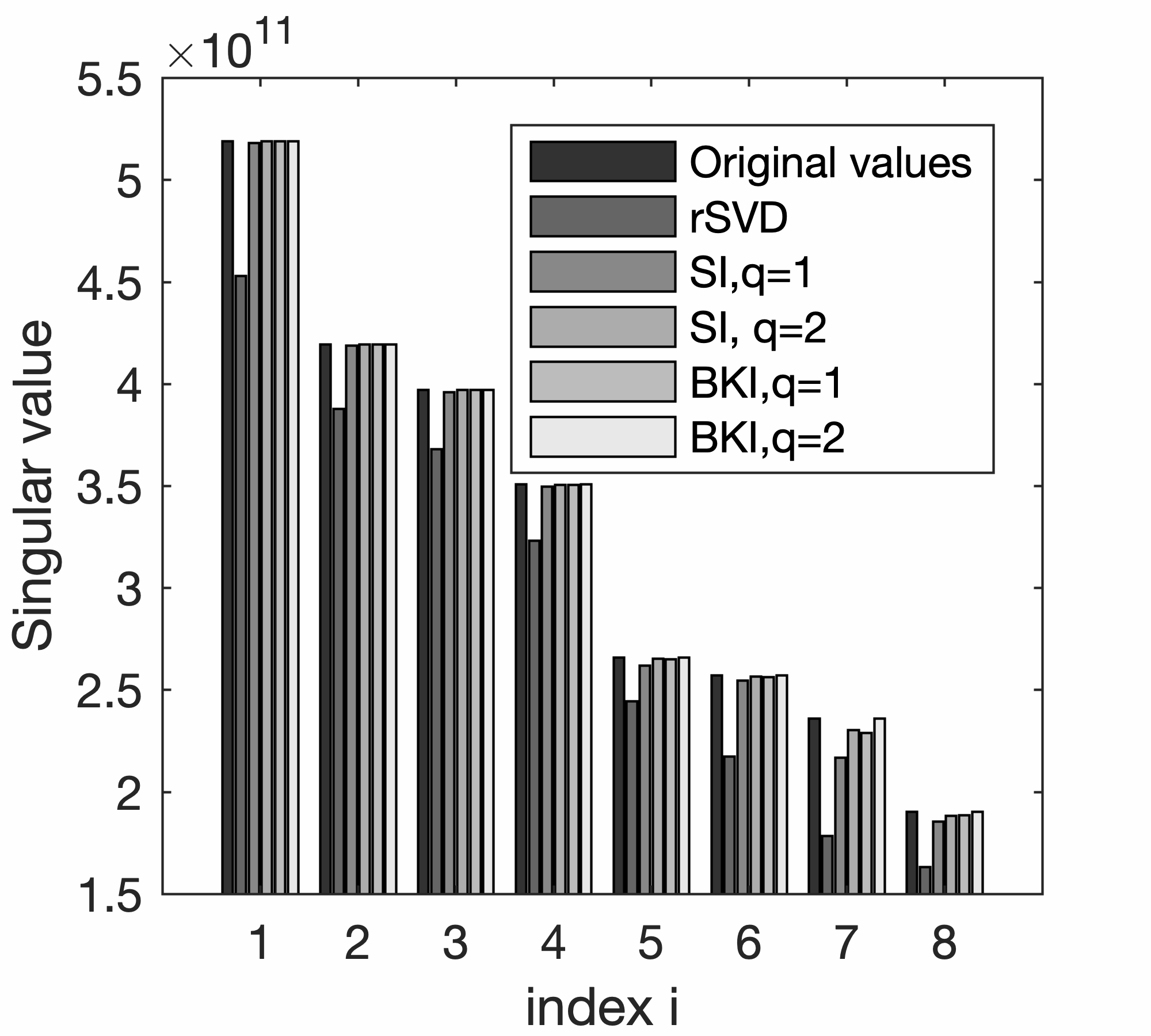
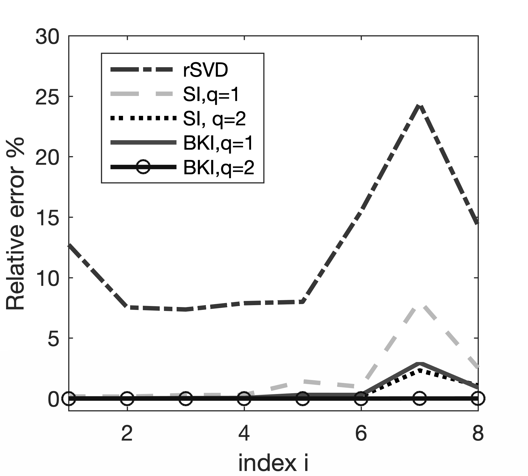
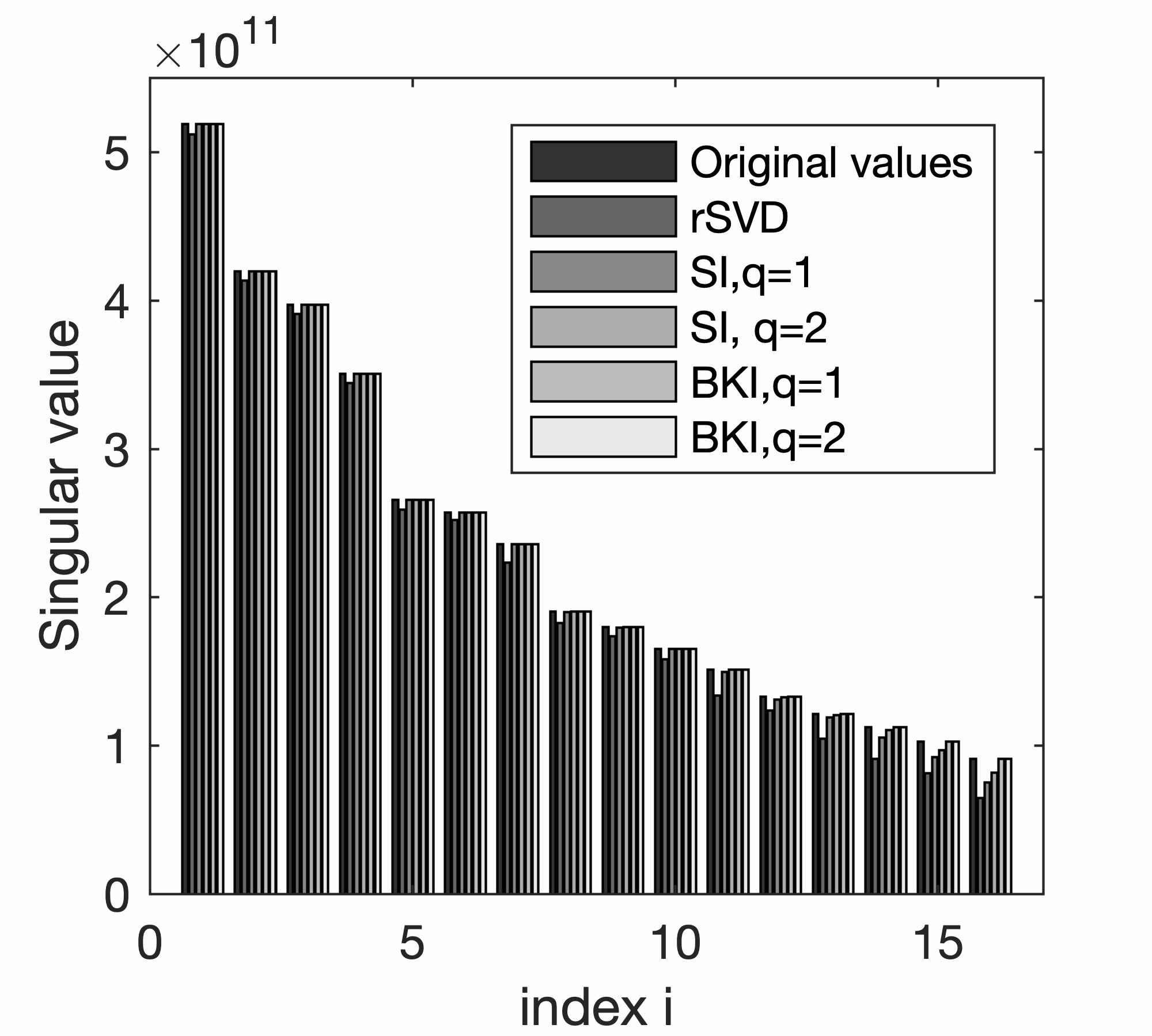
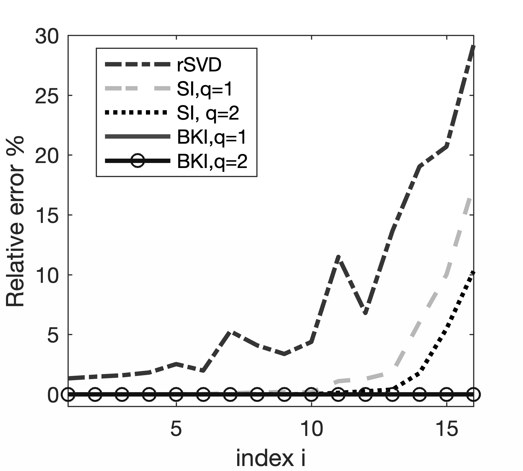
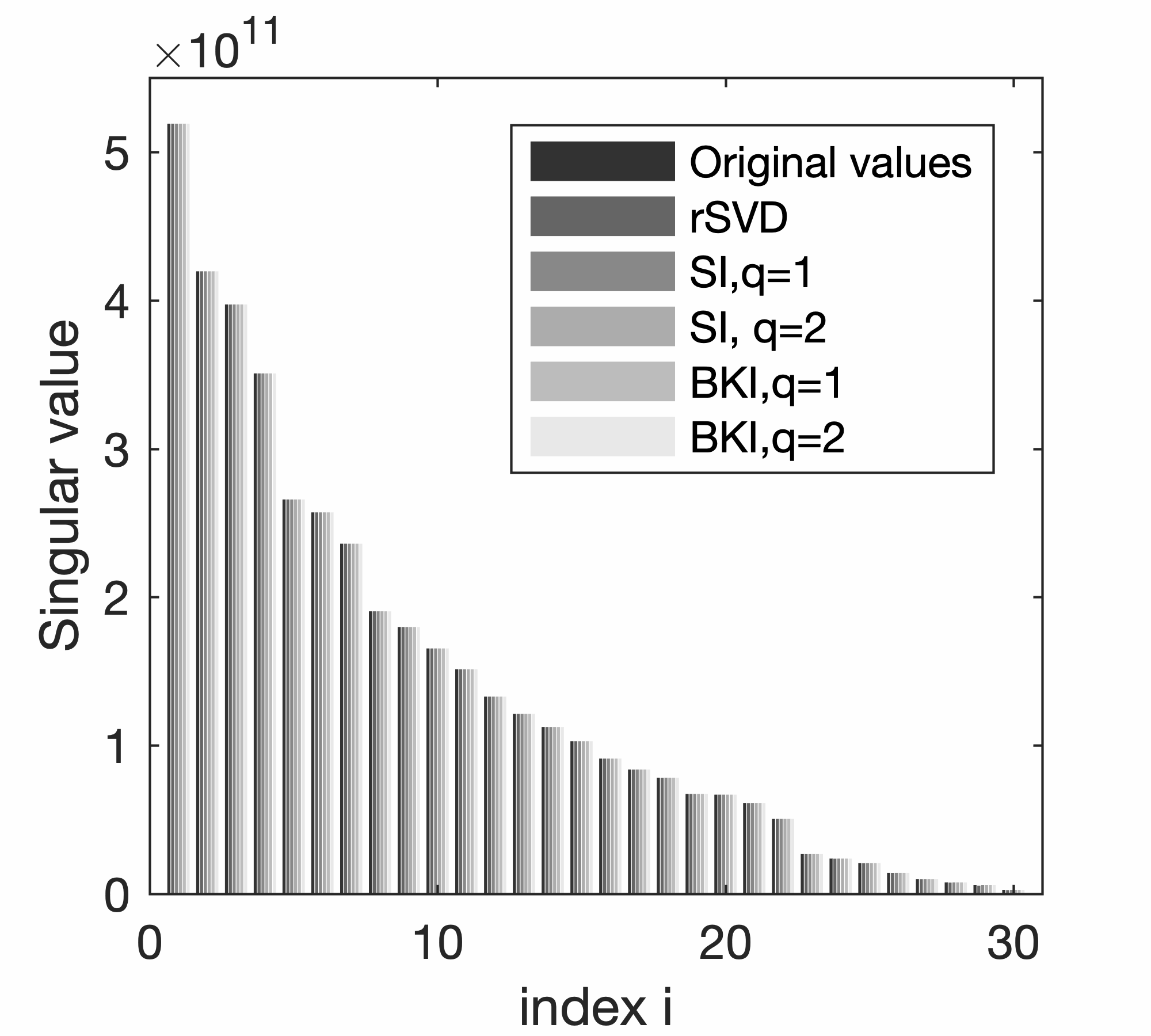
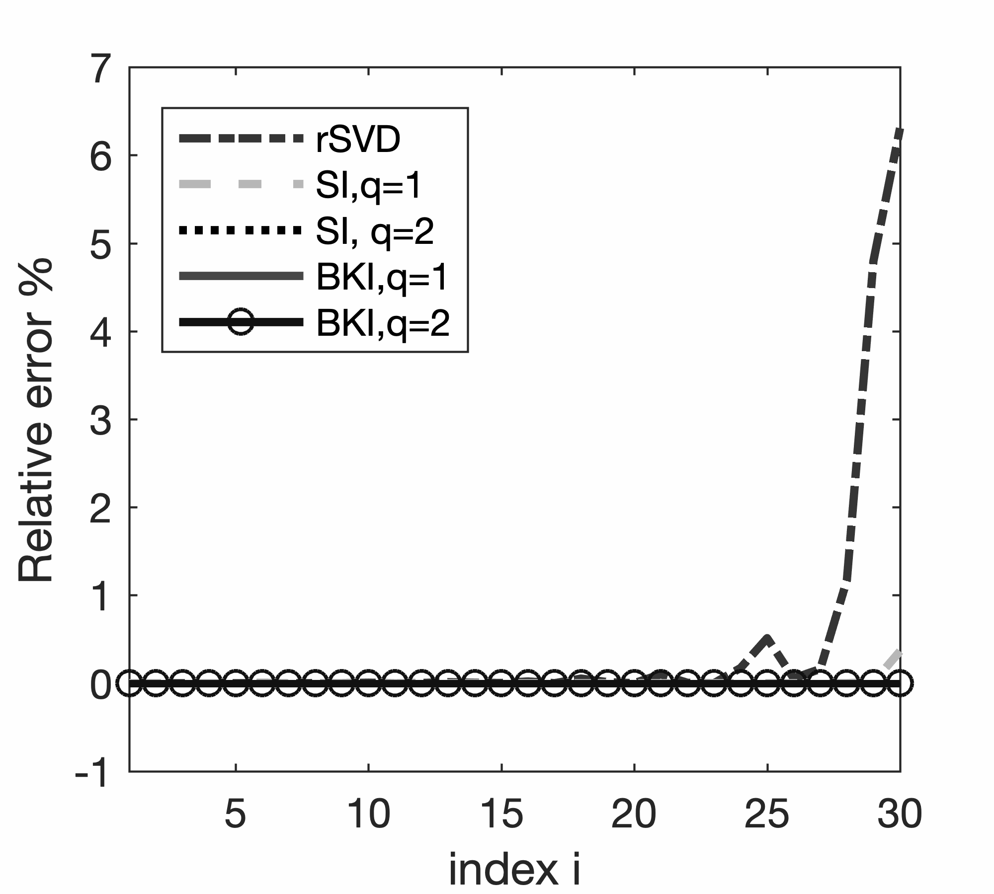
To illustrate the performances of SI and BKI compared to those of conventional rSVD, we conduct additional experiments on a small \(25 \text{Hz}\) monochromatic frequency slice of the EIV included in Figure 2. Because this example is small, we are able to explicitly form the EIV itself and compute its factorization via a conventional SVD. Numerical results are summarized in Figure 5, which displays a plot of the first \(n_p\) singular values for factorization based on probings with \(n_p=8,16,30\). A comparison of the bar plots in Figure 5a, 5c, and 5e leads to the following observations. First, inaccuracies in the estimates for the singular values are greater with a large truncation error, that is, when a substantial amount of energy remains in the tail. In this case, the actual singular values (depicted in dark blue) and the singular values obtained by the standard rSVD method differ significantly. These errors are much smaller when factorizations are based on SI and BKI for either \(q=1\) or \(q=2\). Smaller errors in the singular values lead to smaller errors in the factorization. The plots of the relative errors in Figure 5b, 5d, and 5f show a rapid increase towards the smaller singular values. Even for a probing size \(n_p\) as high as \(30\) where only \(0.4\%\) of the total energy is left in the tail, the relative error for the \(30\text{th}\) singular value calculated by rSVD exceeds \(7\%\) . Both SI and BKI power methods accurately recover the singular values and decrease the relative errors. On the other hand, for a very small probing size of \(n_p=8\), where \(11.4\%\) of the energy in the tail remains, the BKI method with power \(q=2\) recovers the first \(n_p\) singular values with much smaller errors, while SI with power \(q=1,2\) leaves errors in the recovery. Finally, for \(n_p=16\), the remaining energy in the tail decreases to \(5\%\), and the BKI recovers the \(n_p\) singular values very well with \(q=1,2\). We also find that BKI with \(q=1\) recovers the \(n_p\) singular values more accurately than SI with \(q=2\). In summary, both the SI and BKI methods help in decreasing the relative errors in the singular values. Nevertheless, with the same probing size \(n_p\) and power \(q\), BKI always outperforms the other methods.
Typically, BKI with \(q=1\) satisfies the requirement of accurate recovery of the first \(n_p\) singular values. As Figure 6 shows, the errors in the RTM recovered by the rSVD method (cf. Figures 6a and 6b) for \(n_p=8\) are more obvious than those from the BKI with \(q=1\) (cf. Figures 6a and 6c). For the rSVD, coherent energy is lost (cf. Figures 6d and 6e that contain difference plots with respect to the conventional SVD plotted in Figure 6a ). Only the first eight singular values are used in this experiment—i.e., \(n_p=8\ll n_s\) with \(n_s=100\).


Slicing and dicing
Now that we have established a method of factorizing EIVs based on randomized probing with time-domain propagators, we will discuss how to extract various gathers without having to explicitly form the EIVs themselves (see also Da Silva et al. (2019), who accomplishes the same when using a tensor factorization based on the hierarchical Tucker format). Aside from having major advantages regarding memory use and storage, all described operations scale with the rank of the factorization, and as long as this rank \(k< \frac{n_s}{4}\), we benefit computationally compared to methods that loop over shots. In addition, after factoring the EIVs, no additional wave-equation solves are needed to extract the gathers. Three different gathers will be considered, namely Common Image Point gathers (CIPs), Common Image Gathers (CIGs), and geologic dip-corrected CIGs. The latter correspond to CIGs that entail computation of the subsurface offset in the direction parallel to the geologic dip. As outlined by van Leeuwen et al. (2017), including this rotation has advantages for amplitude-versus-offset analyses. We will also show that it leads to improved focusing.
To set the stage, we use the following notation for the discretized image volume \(\mathbf{E}[i_z,i_x;j_z, j_x]\) with \(i_z=1\cdots n_z\), \(i_x=1\cdots n_x\), the indices along the spatial coordinates (using the column-major convention where the first index indicates the rows) and with \(j_z=1\cdots n_z\), \(j_x=1\cdots n_x\), the indices that run over the second set of coordinates. For notational simplicity, the frequency index is dropped. By summing over different gathers for each frequency, the zero-time imaging condition is imposed.
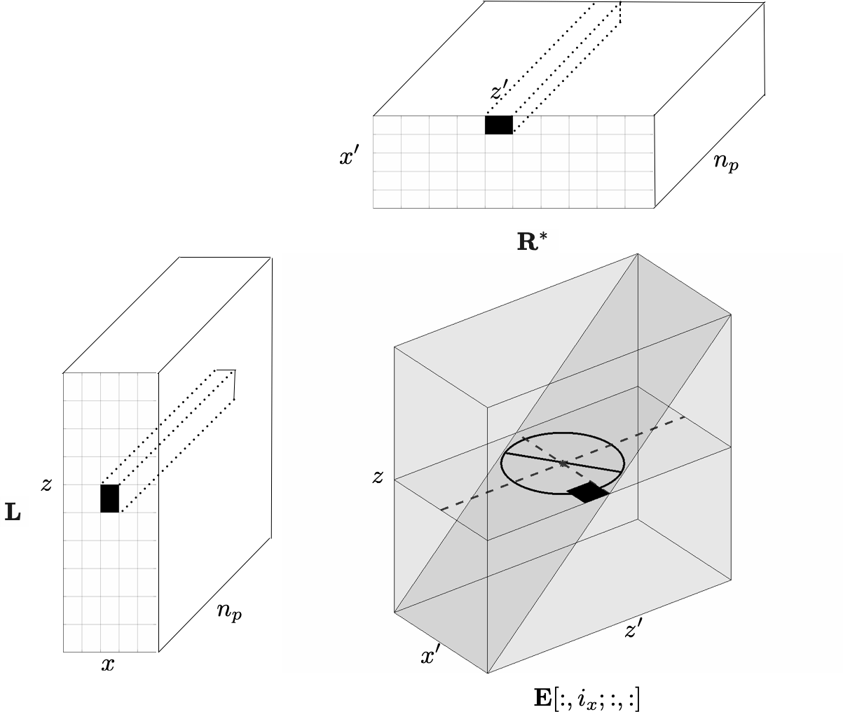
While formally a matrix of size \(N\times N\), the discretized image volume can be considered as a four-dimensional array. Similarly, the factors can be regarded as multi-dimentional arrays—i.e., we have \(\mathbf{L}[i_z,i_x;i_p]\) with \(i_p=1\cdots n_p\) and \(\mathbf{R}[j_z,j_x;i_p]\) as depicted in Figure 7a). However, whenever we operate on the factors we consider them as matrices of size \(N\times n_p\), so they can be multiplied. To extract vectors or matrices from these multi-dimensional arrays, the symbol \(:\) is introduced and refers to all entries along the corresponding dimension.
According to van Leeuwen et al. (2017), a CIP gather indexed by a single point \((i_z,i_x)\) is given by the following 2D slice \(\mathbf{E}[i_z, i_x;\, :,\,:]\), indicated by the horizontal plane in Figure 7b. To avoid forming EIVs explicitly, we implement the extraction of CIPs directly from the factors as performed in Algorithm 3. By applying this algorithm, the vector \(\mathbf{l}=\mathbf{L}[i_z, i_x;\,:] \in \mathbb{C}^{1\times n_p}\) is extracted, followed by a loop over depth, during which this vector is applied to the transpose of the matrix \(\mathbf{R}[j,\, :;\, :]\in\mathbb{C}^{n_x\times n_p}\) for \(j=1\cdots n_z\).
0. Input: location CIP \((i_z,i_x)\) and low rank factors \(\{\mathbf{L},\mathbf{R}\}\)
1. extract the vector \(\mathbf{l}=\mathbf{L}[i_z, i_x;:] \in \mathbb{C}^{1\times n_p}\)
2. for j=1:\(n_z\)
3. \(\mathbf{E}[i_z,i_x;j,\, :] = \mathbf{l} \mathbf{R}^*[j,\, :;\, :]\)
4. end
5. Output: Real part of \(\mathbf{E}[i_z,i_x;\, :,\, :]\)
CIG gathers for the horizontal subsurface offset correspond to taking out \(\mathbf{E}[i_z,i_x;j_z=i_z,\, :],\quad i_z=1 \dots n_z\), as depicted by the inclined plane in Figure 7b. Algorithm 4 extracts CIGs along all depths and at a single lateral index \(i_x\), by taking out the vector \(\mathbf{l}=\mathbf{L}[j,i_x,\, :]\in \mathbb{C}^{1\times n_p}\) within the loop over the vertical coordinate, followed by a multiplication with the matrix \(\mathbf{R}^\ast[j,\, :;\, :]\). The resulting CIG correspondes to the real part of \(\mathbf{E}[i_z,i_x;j_z=i_z,\,:]\) for \(i_z=1\cdots n_z\).
0. Input: lateral index of the CIG \(i_{x}\) and low rank factors \(\{\mathbf{L},\mathbf{R}\}\)
1. for j=1:\(n_z\)
2. extract the vector \(\mathbf{l}=\mathbf{L}[j,i_x;\, :] \in \mathbb{C}^{1\times n_p}\)
3. \(\mathbf{E}[j,i_x;j,\, :] = \mathbf{l} \mathbf{R}^\ast[j,\, :;\, :]\)
4. end
5. Output: Real part of \(\mathbf{E}[i_z,i_x;j_z=i_z,\, :]\) for \(i_z=1\cdots n_z\)
In addition to CIPs and CIGs, geologic dip-corrected CIGs can be formed, which combine information from both gathers by estimating the geologic dip as a function of depth along the CIG. This geologic dip is calculated by maximizing the stack power of CIPs. As shown by van Leeuwen et al. (2017) and Biondi and Tisserant (2004), CIGs computed with horizontal offsets poorly focus when reflectors are steeply dipping. According these authors, there is a complete lack of focusing of vertical reflectors when using horizontal subsurface offsets. The same applies to horizontal reflectors when using vertical subsurface offsets. Following the work, we compute the geologic dip and subsequently correct for this dip so that the selected subsurface offset direction is always parallel to the geologic dip. Our approach differs from recent work (Dafni and Symes, 2016b, 2016a) because we rely on cheap access to CIPs for each depth level without the need to carry out expensive cross correlations on spatio-temporal wavefields. Our method also does not require additional wave-equation solves and excessive storage.
Invariance relationship of EIVs
So far, we have focused on finding representations for EIVs using factorizations informed by randomized probings. Our factorizations incur an upfront cost dominated by the number of randomized probings that determines the number of wave-equation solves. All subsequent manipulations, such as forming CIPs and (angle corrected) CIGs, do not involve wave-equation solves, so they are relatively inexpensive. Moreover, the number of probing vectors is often smaller than the number of source experiments, i.e., \(n_p\ll n_s\).
To allow for more realistic imaging workflows, during which various imaging scenarios are conducted involving different background velocity models, we leverage an important invariance property of EIVs. This invariance of the double two-way wave equations, which model EIVs, allows us to carry out velocity continuation (van Leeuwen and Herrmann, 2012; Kumar et al., 2018)—i.e., to directly map an image volume obtained for one background velocity model to an image volume yielded by another background velocity model without the need to remigrate involving a loop over \(n_s\) shots. To arrive at this formulation, this invariance of the double two-way wave equation is applied directly to the low-rank factorizations of EIVs as introduced earlier. Since \(n_p\ll n_s\), this formulation allows for imaging with varying background velocity models—e.g., for different picks of top salt, at a greatly reduced cost. To firmly establish this possibility, we first introduce the invariance relationship in factored form in the Fourier domain, followed by its time-domain counterpart.
Monochromatic invariance relationship
By using the observation that the right-hand-side of the double two-way wave-equation (cf. equation \(\ref{eq:two-way}\)) does not depend on the background velocity model, van Leeuwen et al. (2017) and Kumar et al. (2018) derive an invariance relationship directly relating image volumes \(\mathbf{E}_1\) and \(\mathbf{E}_2\) that pertain to two different background velocity models \(\mathbf{m}_i,\, i=1,2\) (For simplicity, we abandon the frequency subscript, so the subscript now specifies extended image volumes associated with the velocity models of scenarios \(1\) and \(2\)). According to the double two-way wave equation, these image volumes can be related via
\[
\begin{equation}
\mathbf{H}_1^{*} \cdot \mathbf{E}_1 \cdot \mathbf{H}_1^{*} = \mathbf{H}_2^{*} \cdot \mathbf{E}_2 \cdot \mathbf{H}_2^*,
\label{eq:invar_double}
\end{equation}
\]
where the Helmholtz operators \(\mathbf{H}_i=\mathbf{H}(\mathbf{m}_i),\, i=1,2\) depend on the two different background velocity models for the two imaging scenarios. This relationship allows us to directly calculate EIV \(\mathbf{E}_2\) for imaging scenario \(2\) from the EIV of imaging scenario \(1\) via the relationship
\[
\begin{equation}
\mathbf{E}_2 = \mathbf{H}_{2}^{-*} \cdot \mathbf{H}_{1}^{*} \cdot \mathbf{E}_{1} \cdot \mathbf{H}_{1}^{*} \cdot \mathbf{H}_{2}^{-*}.
\label{InvForm}
\end{equation}
\]
Since EIVs can be represented in factored form, the factors for both imaging scenarios are also related by
\[
\begin{equation}
\begin{aligned}
\mathbf{L}_{2} &= \mathbf{H}_{2}^{-*} \cdot \mathbf{H}_{1}^{*} \cdot \mathbf{L}_{1}, \\ \\
\mathbf{R}_{2} &= \mathbf{H}_{2}^{-1} \cdot \mathbf{H}_{1} \cdot \mathbf{R}_{1}.
\end{aligned}
\label{eq:factors}
\end{equation}
\]
With this established relationship, EIVs only need to be factored once, i.e., for the velocity model of scenario \(1\). All subsequent factorizations for various imaging scenarios can be derived with equation \(\ref{eq:factors}\), precluding the computationally expensive step of randomized probing, followed by the BKI. As a result, we arrive at a formulation where the factorization costs of EIVs are incurred only once up-front. After the initial factorization, only \(2n_p\) wave-equation solves per factor are needed per factor, which eliminates the computational overhead associated with the initial factorization. This finding is significant in situations where the background velocity model contains uncertainties. In the next section, we will discuss the implementation of these invariance relationships based on time-domain wave-equation solvers.
Velocity continuation in the time domain
The combination of low-rank factorizations with the above invariance relationship enables us to directly form factored EIVs for various velocity models without the need to redo the factorization, including the probing. According to equation \(\ref{eq:factors}\), we need access only to the factors in the current velocity model, the action of the forward and adjoint wave equation in the current and the new velocity model, and the solution to these wave equations for the two velocity models.
While the monochromatic invariance relationship allows for a mapping of the factors from one velocity model to another, the formulation hinges on the action of discrete wave-equation operators and their inverses. Unfortunately, the need for the latter may become problematic since Helmholtz solvers do not scale well to high frequencies and 3D models. To address this issue, we employ wave-equation solvers, including the action of the wave-equation itself and not its inverse, based on time-stepping and finite differences implemented with Devito (Louboutin et al., 2018). Based on this time-domain implementation, the new factors, which now become tensors, can be written as follows: \[ \begin{equation} \begin{aligned} \mathbf{L}_2 &= \mathcal{F} \circ \mathcal{A}_2^{-\top} \circ \mathcal{A}_1^{\top} [\mathsf{L}_1] \quad & \text{with} \quad & \mathsf{L}_1 = \mathcal{F}^\top [\mathbf{L}_1],\\ \mathbf{R}_2 &= \mathcal{F} \circ \mathcal{A}_2^{-1} \circ \mathcal{A}_1[\mathsf{R}_1] \quad & \text{with} \quad & \mathsf{R}_1 = \mathcal{F}^\top [\mathbf{R}_1]. \end{aligned} \label{eq:factors-time} \end{equation} \] Here \(\mathcal{A}_2^{-1}\) represents forward modeling in velocity model \(\mathbf{m}_2\) for scenario \(2\), and \(\mathcal{A}_2^{ -\top}\) is the corresponding adjoint operator. The linear operator \(\mathcal{A}_1\) is the inverse forward modeling operator for imaging scenario \(1\) with the velocity model \(\mathbf{m}_1\), and \(\mathcal{A}_1^{ \top}\) is the corresponding adjoint operator. As in the monochromatic case, the direct mapping of the factored form of one EIV onto another velocity model involves only \(2n_p\) actions of the forward/adjoint wave equations and their inverses. Note that compared to the frequency domain formulation, the computational costs of the time-domain operators and their inverses is roughly the same while the cost of applying the Helmholtz operator is low compared to applying its inverse.
In addition to reducing the cost (from \(\mathcal{O}(n_s)\) to \(\mathcal{O}(n_p)\) actions with wave operators and their inverses), the main advantage of working with factored EIVs is that we incur only the costs of the initial factorization once, which involves randomized probing and a SVD based on BKI. After this initial cost, factorizations of the EIVs can be performed for various imaging scenarios with different velocity models repeatedly. This is possible because the mapping in equation \(\ref{eq:factors-time}\) preserves the accuracy of the original factorization. We make this claim because the action of the wave-equation operators on their inverses is by definition the identity; that is, if we apply the wave operator to a factor, we will undo possible wave simulation errors, such as numerical dispersion. In view of these properties, we argue the benefits of developing a strategy that requires as few factors (\(n_p\)) as possbile calculated with as high accuracy as possible.
Numerical experiments
In this section, we present carefully selected numerical experiments to demonstrate our ability to represent and manipulate EIVs with low-rank factorizations obtained via randomized probing and BKI. We argue that these factorizations are natural parameterizations for full-subsurface EIVs. We show how to apply these factorizations to a series of imaging problems with an emphasis on how to make informed choices on the rank and the order of the BKI method given computational constraints. As we observed from the example with the explicit EIV calculated from a small subset of the Marmousi model, the BKI method with power \(q=1\) outperforms the rSVD and SI. Therefore, we will employ BKI for \(q=1\) for will be employed for the remainder of the paper.
Our first imaging experiments will be conducted on the Marmousi model and are designed to demonstrate our ability to compute RTM images, CIPs, CIGs, and geologic dip-corrected CIGs, with factorizations obtained from randomized probing and BKI. To establish the accuracy of the proposed method, a comparision is made between true CIPs and CIGs and their approximate counterparts derived from the low-rank factorization without having to form the full EIV. To handle imaging problems with steep dips, we show how to calculate CIGs that correct for the local geologic dips. We conclude by examining a large-scale complex imaging problem with salt. To mimic realistic imaging, we examine a scenario where the background velocity model for the top salt is wrong. We demonstrate that our velocity continuation technique is capable of mapping the low-rank representation from the wrong velocity model to corrected factors that produce a well-focused image without refactorization.
Validation of the factored EIV representation
To verify the validity of the proposed factorization method, a series of imaging experiments are conducted involving the Marmousi model. This model is \(8\) km wide and \(3.2\) km deep and discretized on a \(6\) m \(\times 6\) m grid. The data is acquired from \(650\) co-located sources and receivers positioned at a depth of \(18\) m and sampled with a \(12\) m interval horizontally. Data are simulated with the acoustic constant density wave equation with absorbing boundaries all around and a Ricker wavelet centered \(23\) Hz. Before imaging, the direct wave from the simulated “observed” data is removed.
As illustrated previously, the quality of the factorization of EIVs depends on the probing size \(n_p\), which also determines the computational cost. To choose a value for the probing size, we plot in Figure 8 the rank of the SVD we need to capture \(95\%\) of the energy in the observed data. According to this plot, the observed data need to be approximated with a rank \(266\) factorization to reduce the error to \(5\%\). As observed in Figure 4, the singular values of EIVs decay roughly twice as fast suggesting \(n_p=130\) for the factorization with BKI and \(q=1\).
Given this factorization, we compute a migrated image via equation \(\ref{eq:RTM-diag}\) for comparison with a regular RTM image computed over all \(n_s=650\gg 130\) sources. Aside from some noise, the migrated images obtained from the factorization and conventional RTM are close (cf. Figure 9b and 9a). Although the quality of the extracted RTM from the recovered low-rank factorization of the EIV is high, the image as shown by Figure 9 is not perfect due to the loss of energy in the singular values beyond the \(130^\text{th}\) singular value. Since the factorization is approximate, the image is somewhat noisy and has slightly less well resolved amplitudes. However, this is not surprising because the factorization is approximate with an error that can be controlled by increasing \(n_p\). Nevertheless, this slight image deterioration is a relatively small price to pay compared to the benefit of having access to full subsurface offset image volumes that include information on the underlying scattering mechanism and the quality of the velocity model. This information can be calculated without the need to compute additional wave-equation solves.
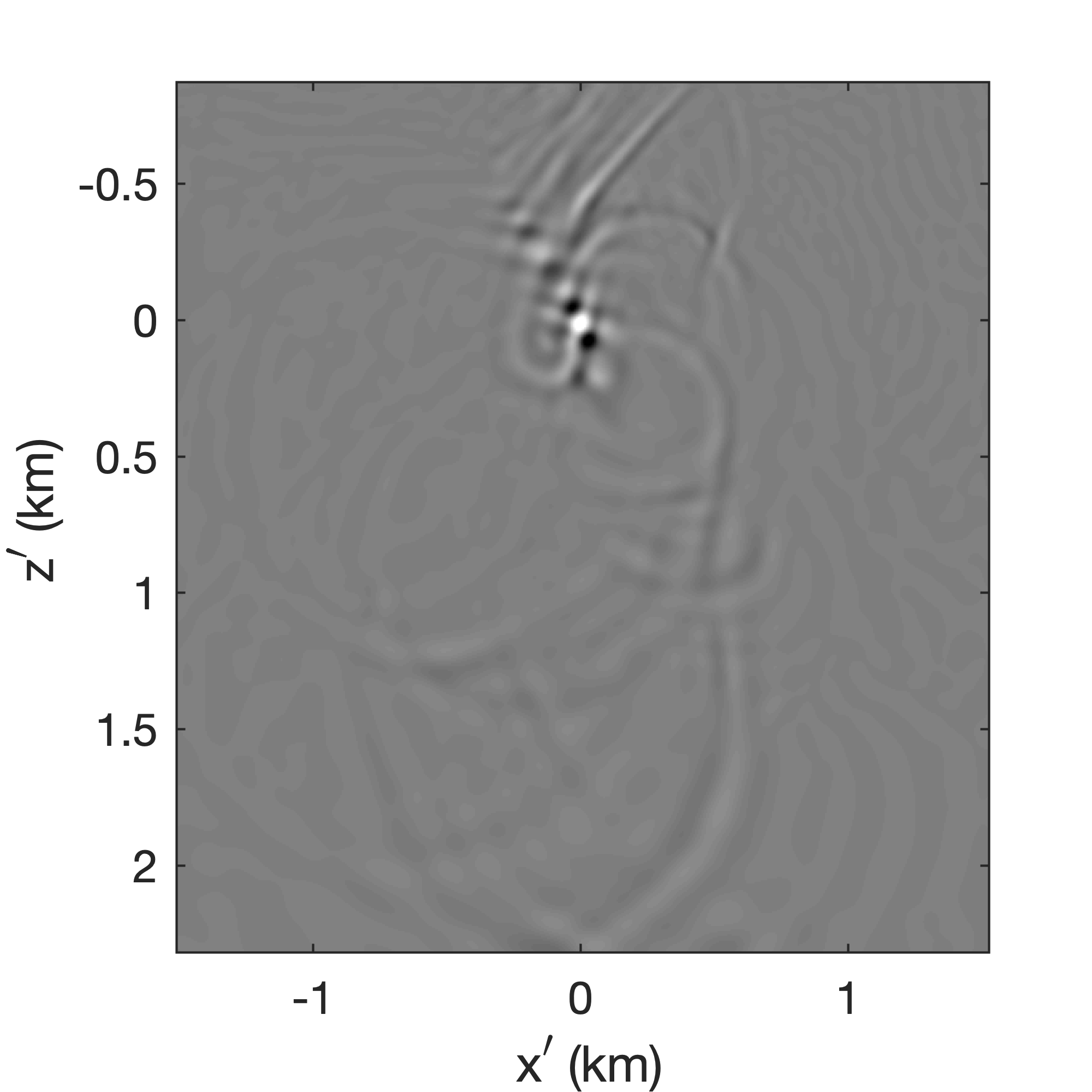
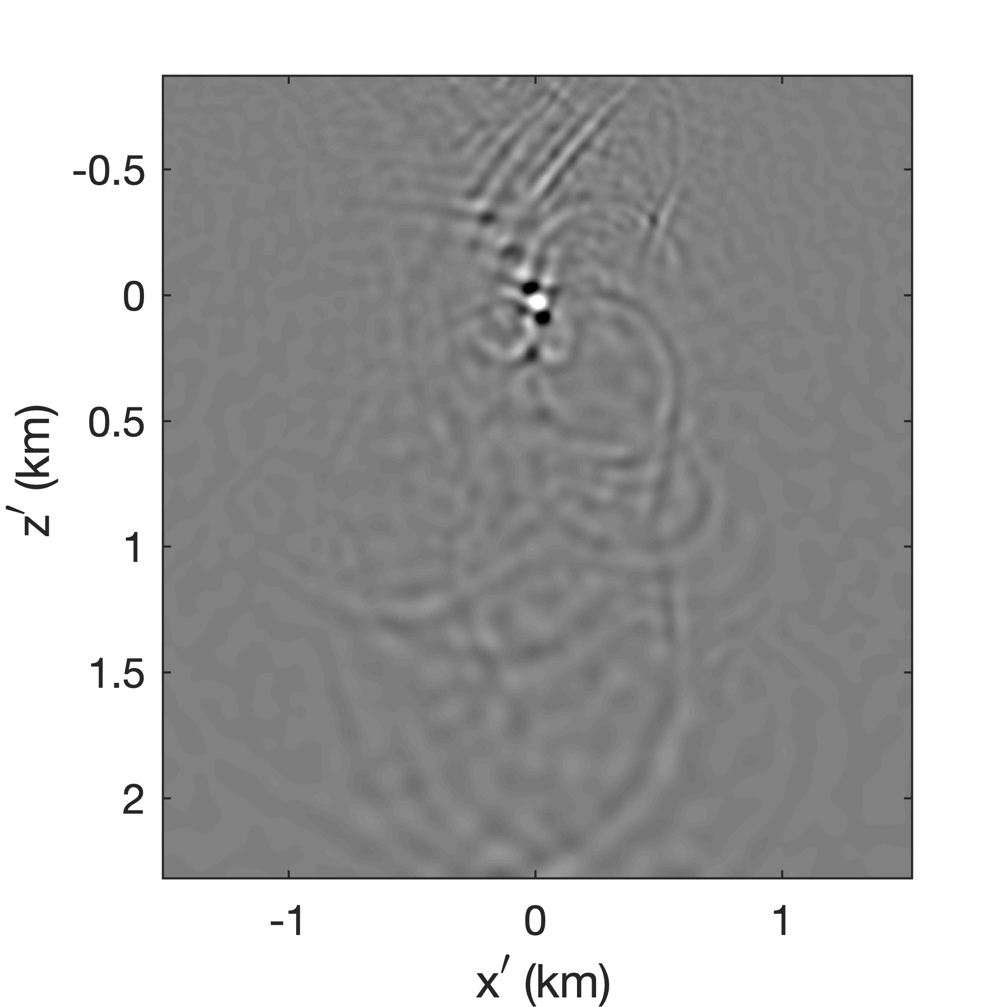
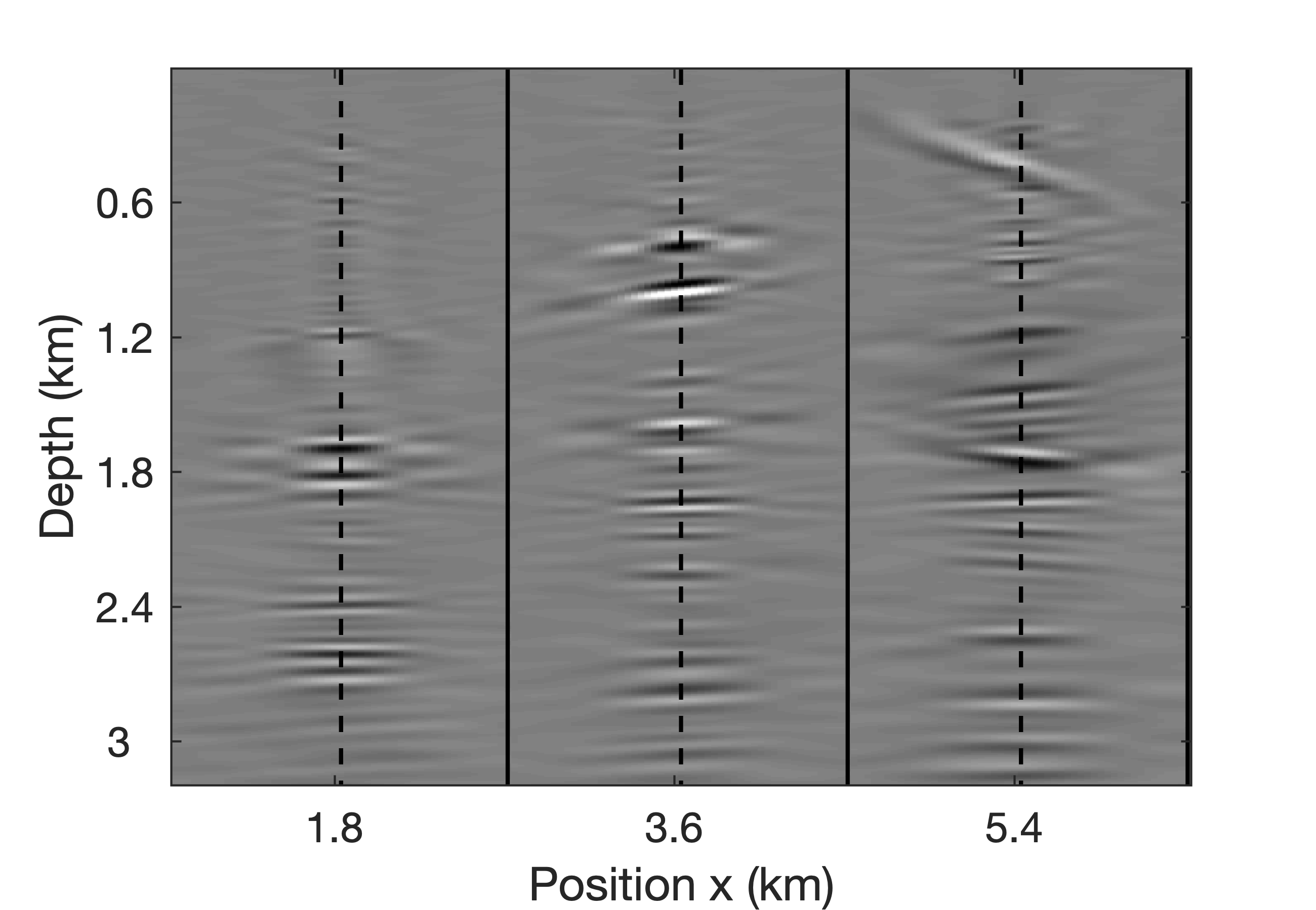
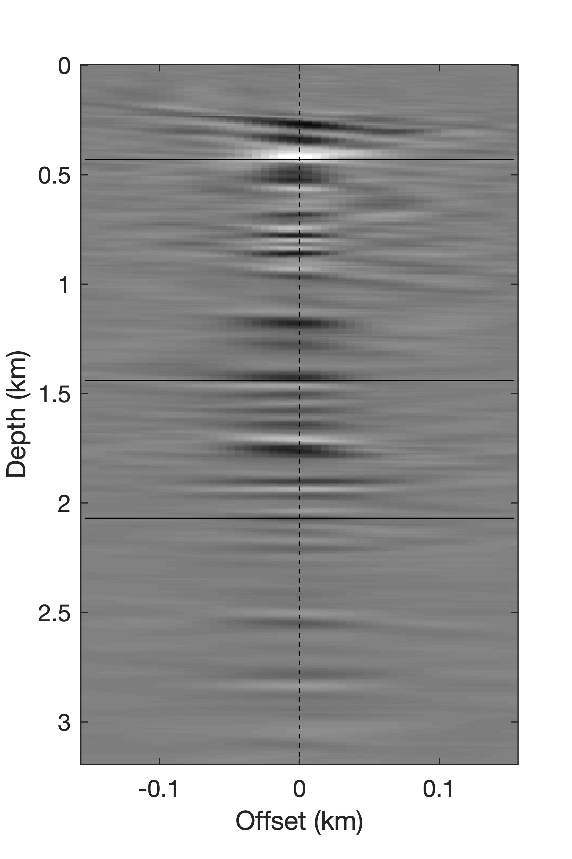
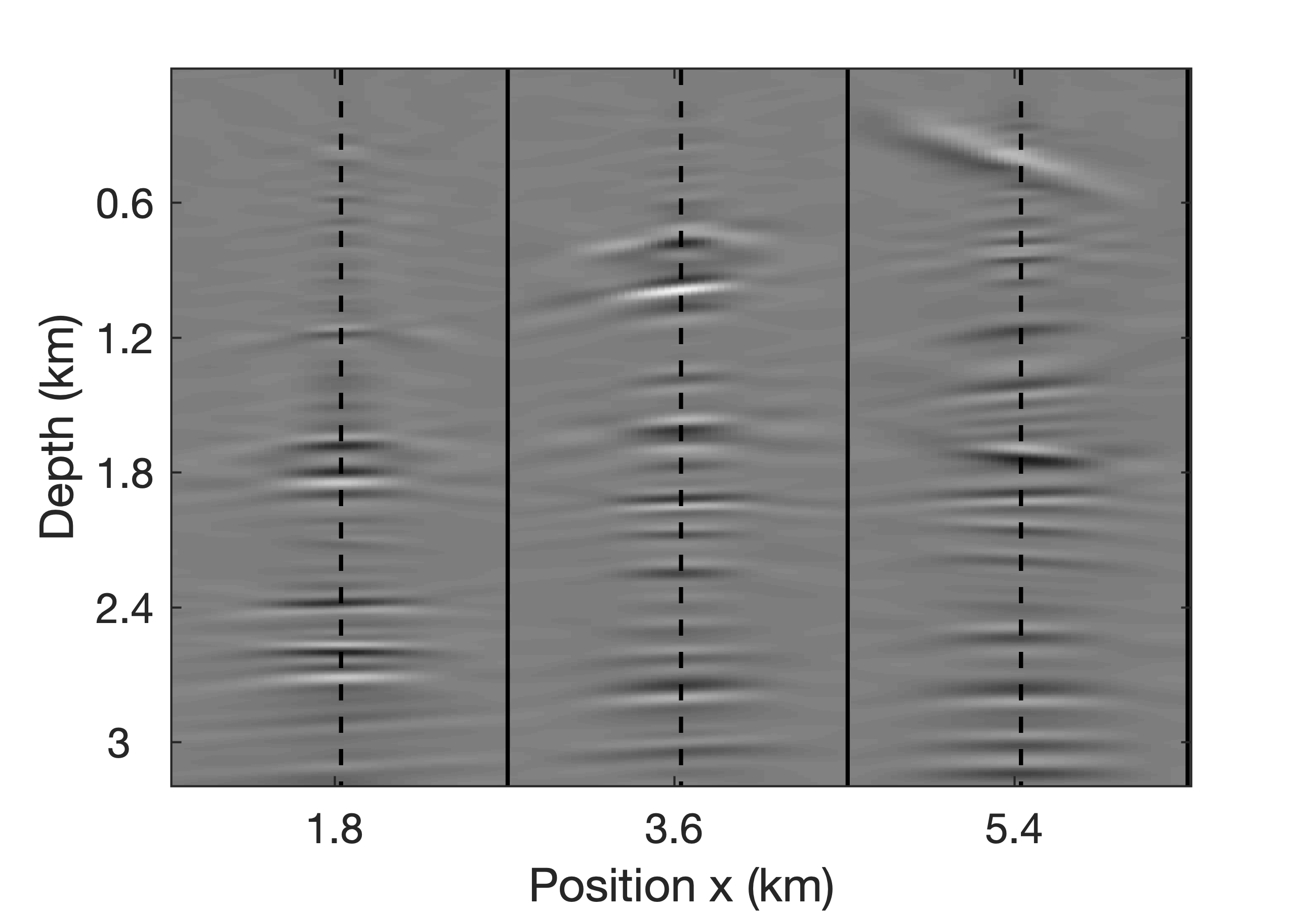
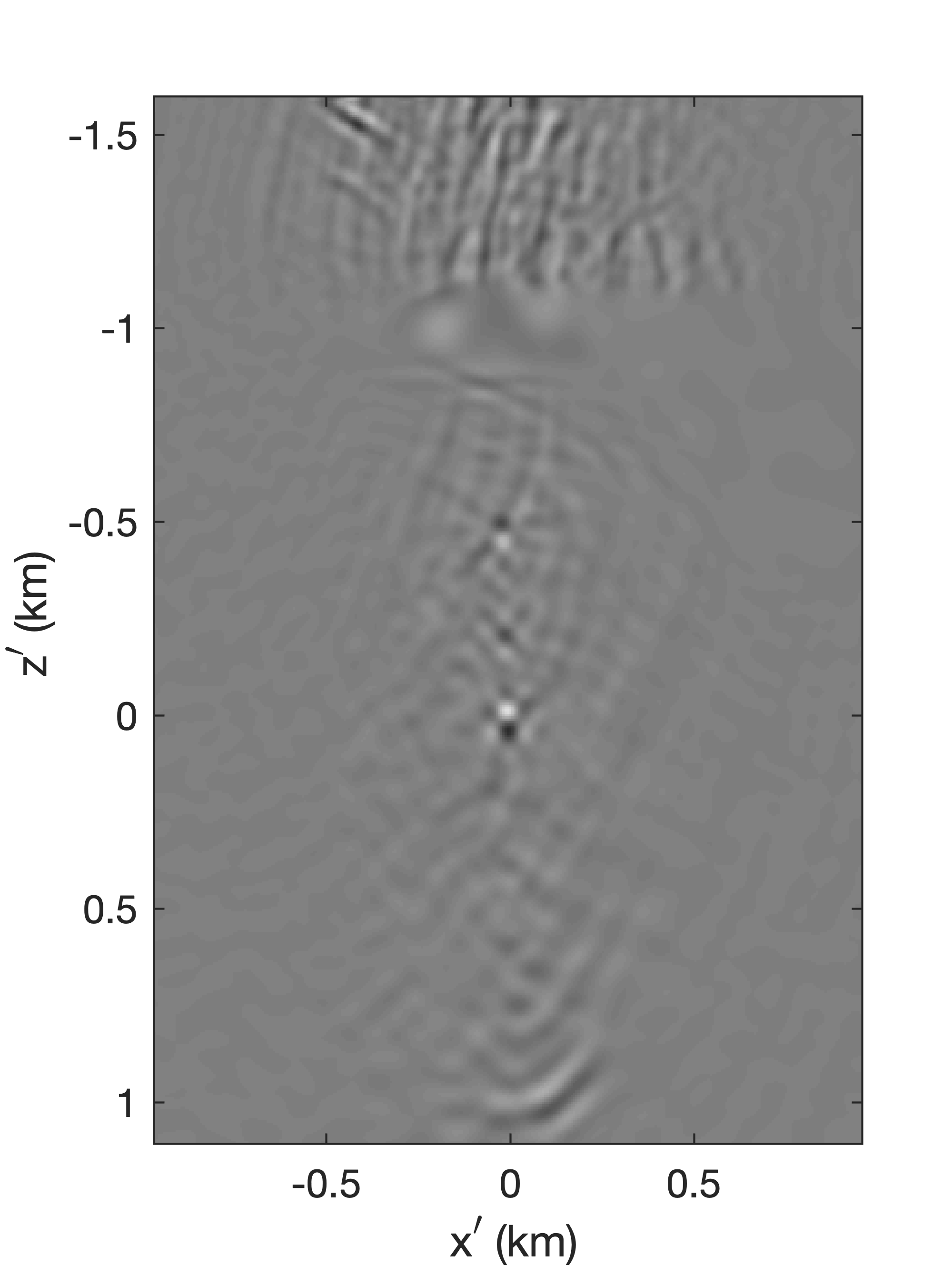
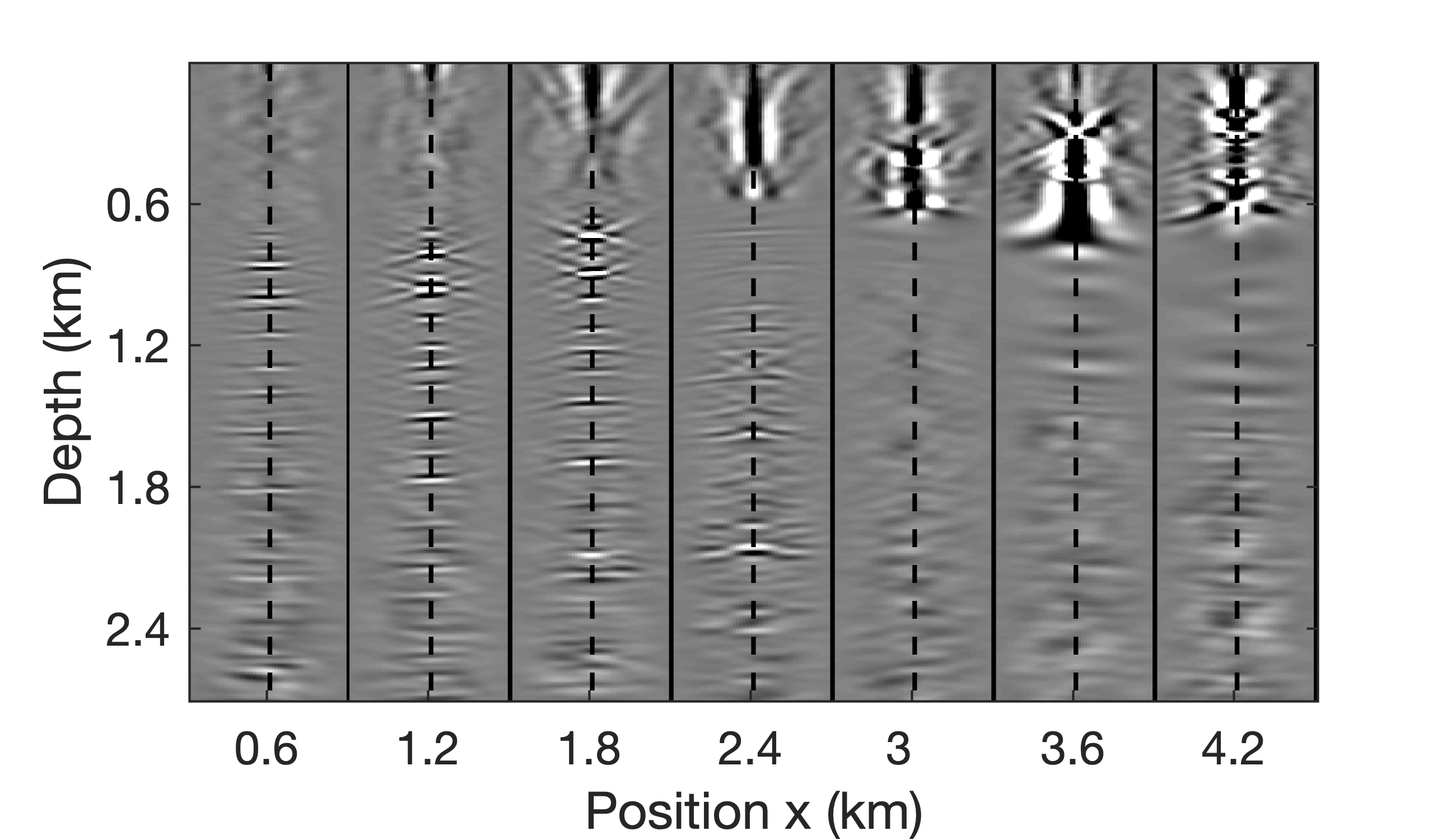
To demonstrate access to full-subsurface-offset gathers, a comparision is made in Figure 10 between a true CIP, obtained by the time-domain probing of the EIV with a single bandwidth-limited point source located at \((z=870\mathrm{m}, x=5250\mathrm{m})\) (for details, see van Leeuwen et al. (2017)), and a CIP computed from the factors using Algorithm 3. As with the RTM image itself, the CIP derived from the factors, albeit noisy, captures most of the energy. As with the true CIP, the approximate CIP shows a clear directivity pattern with a rotation that is consistent with the geologic dip. Remember that the approximate CIP does not require additional wave-equation solves. Finally, we also include comparisions for three CIGs located at \(x=1.8, 3.6, 5.4\)km over an offset range from \(-150\) to \(150\)m. Figure 11 juxtaposes true CIGs and their approximations computed from the factorization with Algorithm 4. As before, the approximate CIGs are consistent with the true CIGs. Except for the presence of some noise, the approximate CIGs (Figure 11b) capture the behavior of the true CIGs (Figure 11b). As expected, the energy is well focused for flat reflectors because the background velocity model is kinematically correct. All approximate results are computed from a factorization with the BKI method for \(q=1\) and \(n_p=130\).


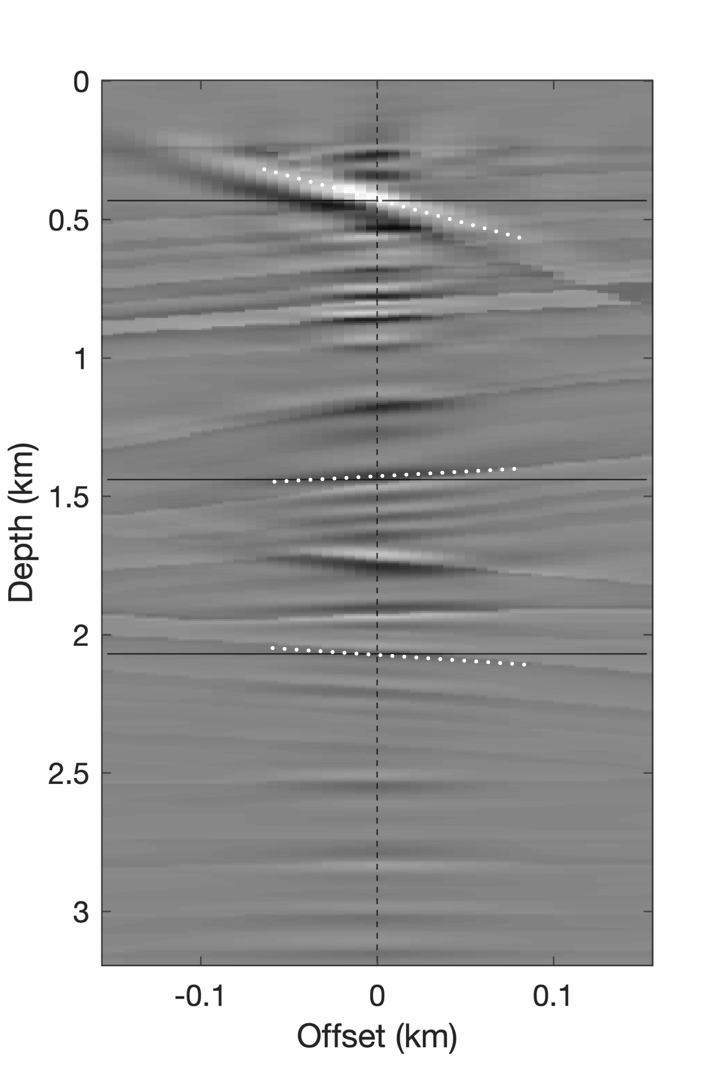
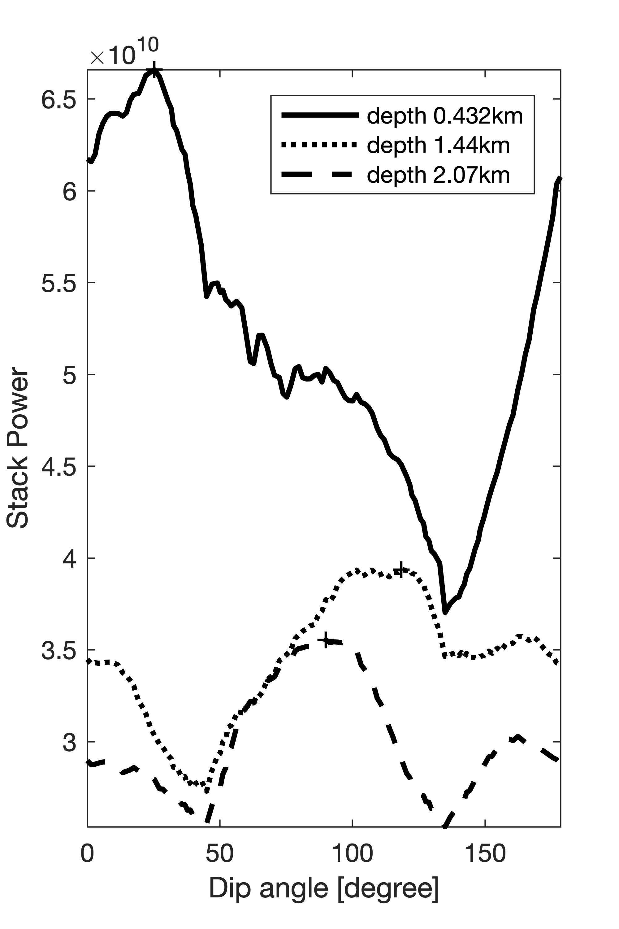
To improve the focus of CIGs for steeply dipping reflectors, we apply dip-corrected CIP at \(x=5.4\) km. This correction compensates for geologic dips so that the subsurface offset is always in the direction parallel to the specular reflector. As Figure 12a shows, the focus of the CIG is not clear in locations where the geologic dip is steep. By computing the stack power of CIPs for each depth level along lines with various angles this dip can be estimated. As plotted in Figure 12 for three different depth levels, the stack power is maximum when the angle is close to that of the geologic dip. Using the angles with maximum stack power, the geologic dip can be corrected by rotating the direction of the subsurface offset by \(90^\circ\) with respect to the angle where the stack power is maximum. The dashed white lines in Figure 12a correspond to the estimated geologic dips, which are close to the true geologic dips. The CIG computed with this correction is included in Figure 12c. Compared to the original CIG in Figure 12a, the focus of the corrected CIG is much clearer in areas with steep geologic dips.
The above examples demonstrate the capability of our factored formulation to acquire accurate imaging results. In addition to approximating RTM images well, the factored formulation also provides rapid access to CIPs and (dip-corrected) CIGs without additional wave-equation solves or expensive cross-correlations between spatio-temporal wavefields. This is made possible by working with the low-rank factored form without forming the full EIVs.
Robustness with respect to additive noise
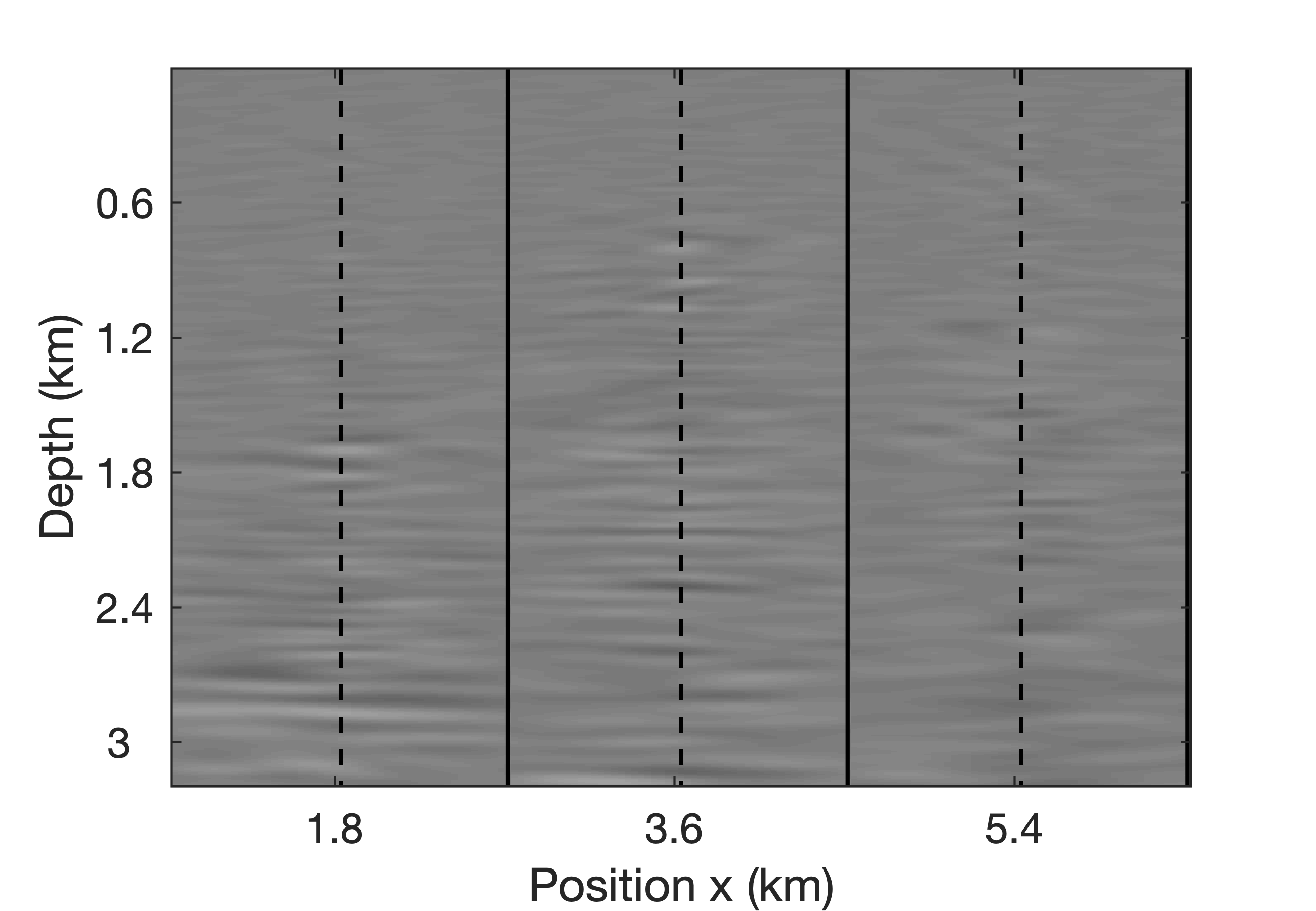
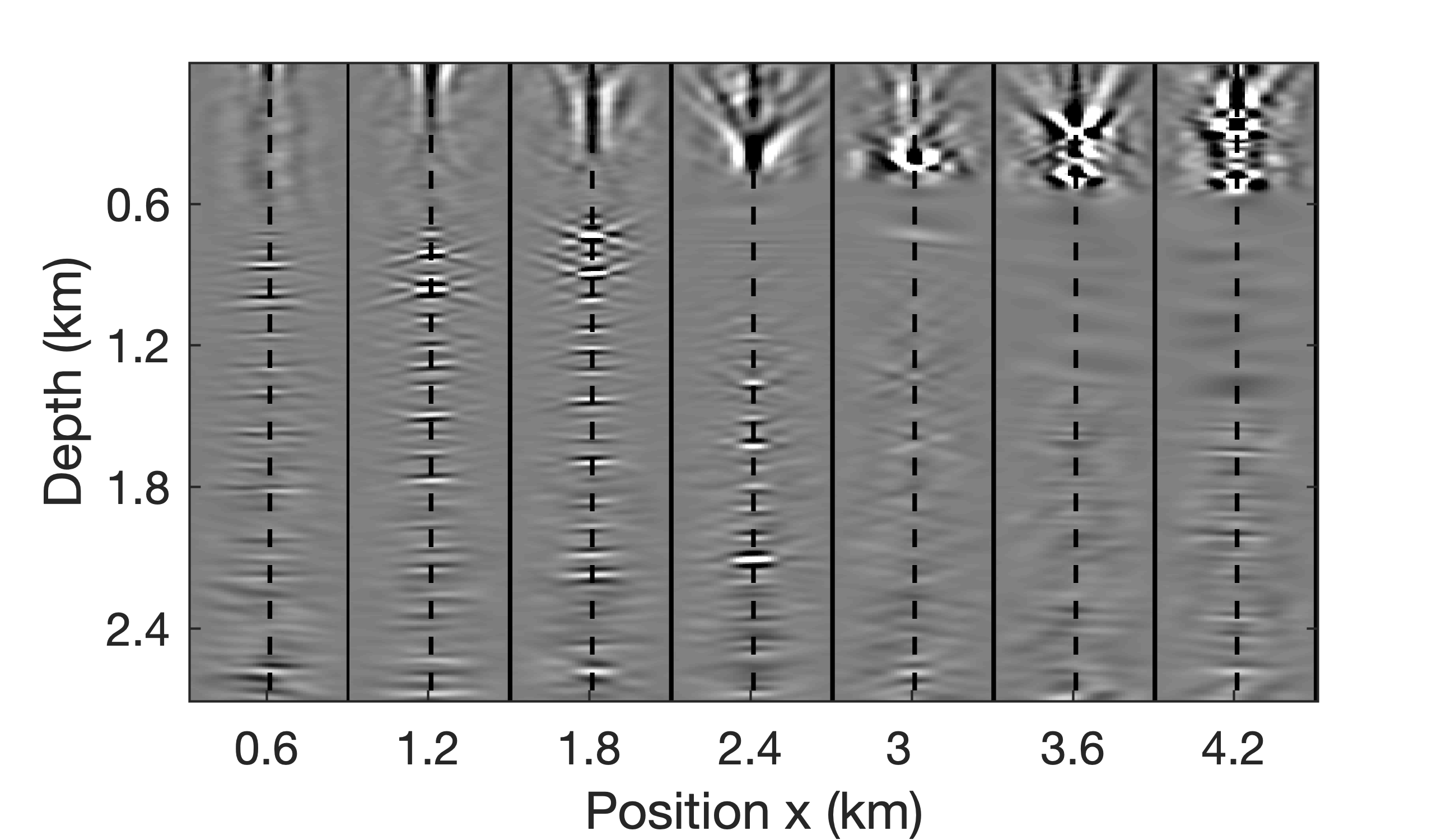
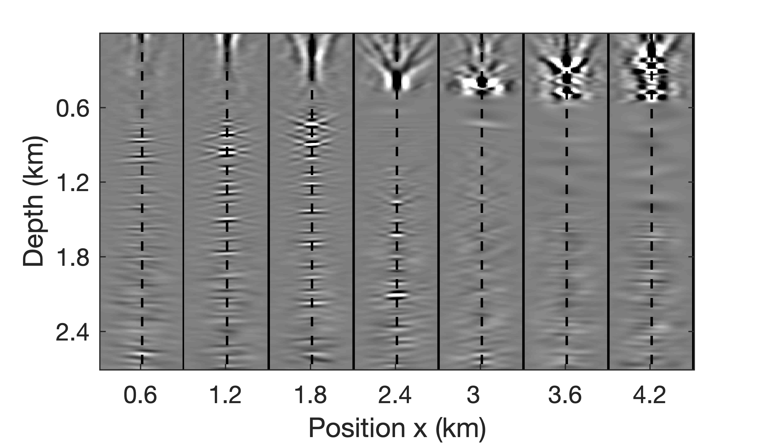
So far, we assume ideal noise-free data. To test the robustness of our low-rank factorization with respect to noise, we add band-limited noise with an energy equal to \(50\%\) of the data’s energy, resulting in SNR of 6.02. Approximate CIGs derived from the low-rank factorization for the noisy data, and their differences with respect to the noise-free case plotted in Figure 11b, are included in Figure 13. From this figure we observe that additive noise has a relative minor effect on the CIGs, a behavior that is consistent with migration where incoherent noise is known to “stack out”.
Salt imaging scenario
Although EIVs in factored form provide us with access to accurate RTM images and subsurface-offset gathers at limited costs, imaging in complex areas remains challenging because of inaccuracies in the background velocity model. For instance, errors in top salt can result in a rapid deterioration of the imaging quality beneath the salt. In practice, this means that imaging teams must go through several cycles of updating the velocity model, followed by imaging. Thus, by using the invariance relationship for EIVs, we propose to use a velocity-continuation technique instead. This technique is based on our factorization method and captured by equation \(\ref{eq:factors}\). By applying these formulas, the left and right factors of one velocity model can be mapped directly to those of another background velocity model without the need to recompute the factorization. In this way, we incur a cost of \(4n_p\), which is relatively small when \(n_p\) is small. Also, these costs are much smaller than a conventional imaging requiring loops over shots.
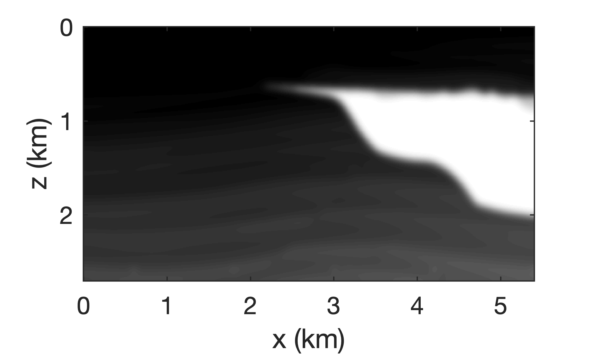
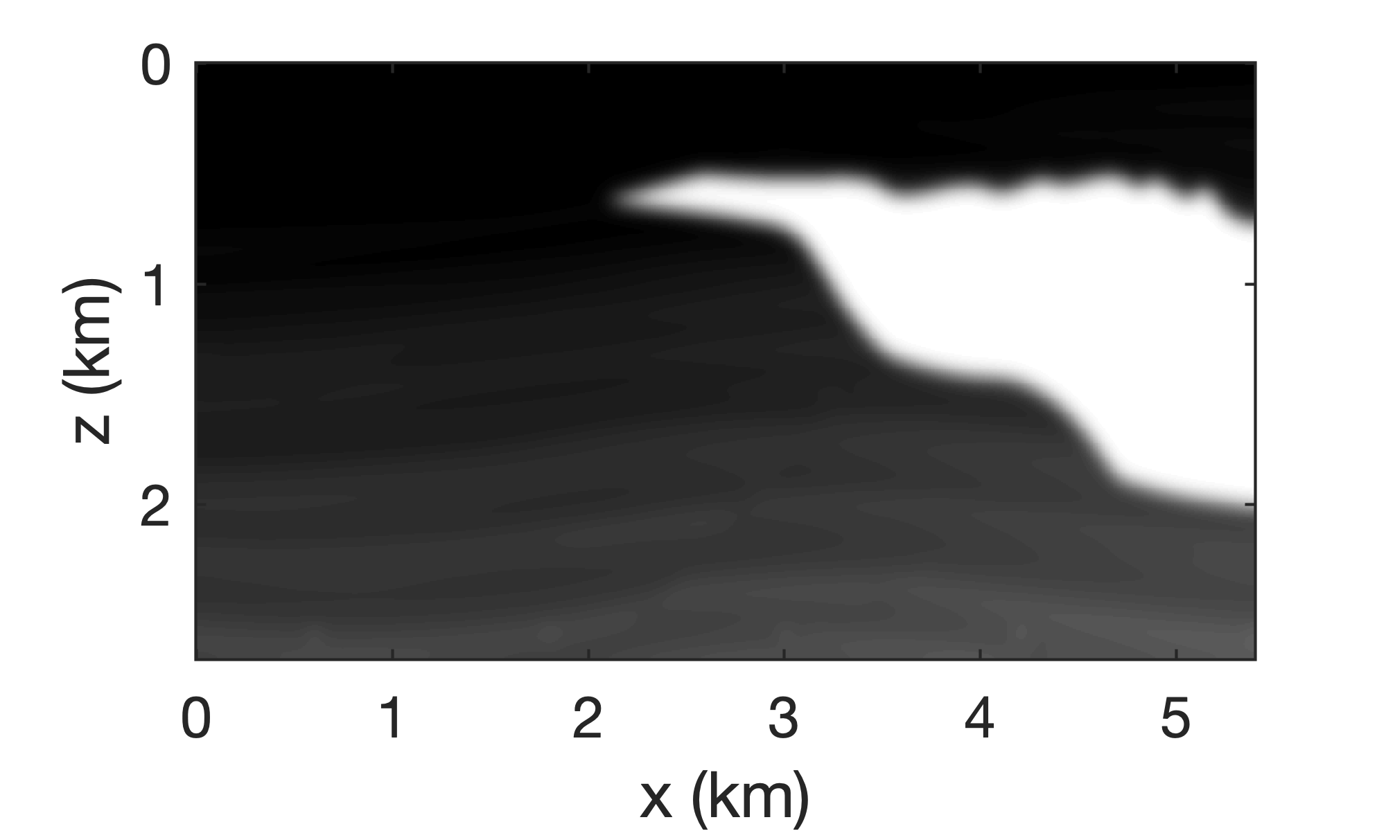
To mimic a realistic subsalt imaging scenario, we compare three scenarios that derive from a subset of the Sigsbee model (Paffenholz et al., 2002). In the first scenario, an image for a background velocity model is computed where the top salt is wrong. We compare this result to that of the second scenario, in which the background velocity model is corrected but from which we remigrate the data by recomputing the factorization. In the third scenario, we use equation \(\ref{eq:factors}\) to compute the image by mapping the EIV in factored form. To avoid salt-related imaging artifacts, the inverse-scattering imaging condition (N. Whitmore and Crawley, 2012, Witte et al. (2017),Crawley et al. (2018)) is used on linearized data simulated from the correct background velocity model depicted in Figure 14b and the true perturbation given by the difference between the \(2.7\)km \(\times 5.4\) km true velocity model and the correct background velocity model, sampled on a \(6\) m \(\times 6\) m grid. Data are simulated for \(450\) co-located sources and receivers spread over the top of the model and located at a depth of \(18\)m sampled with \(12\) m intervals. The source signature is a \(23\) Hz Ricker wavelet.
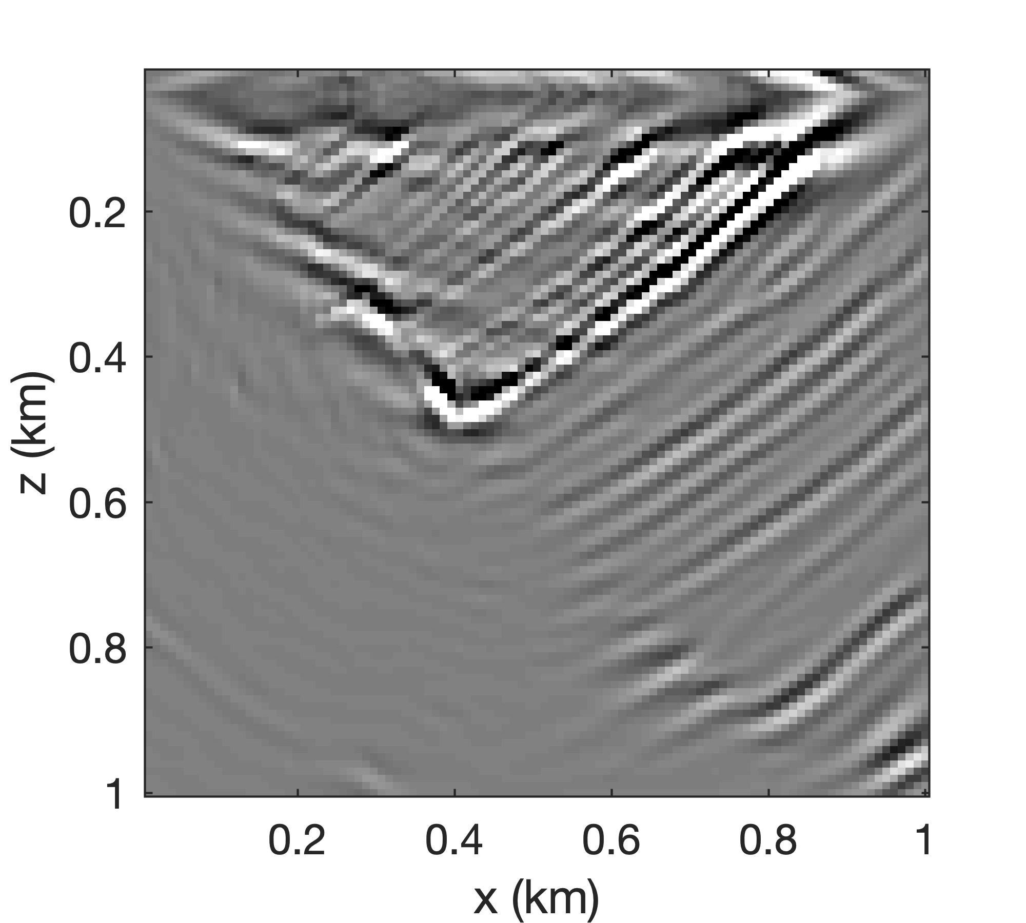
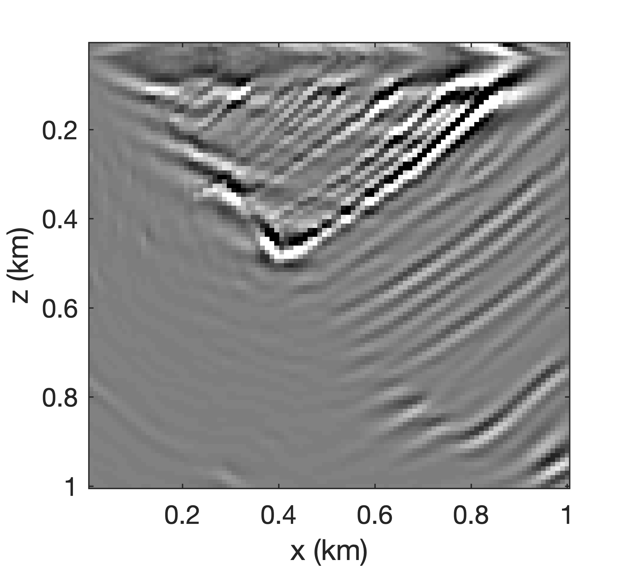
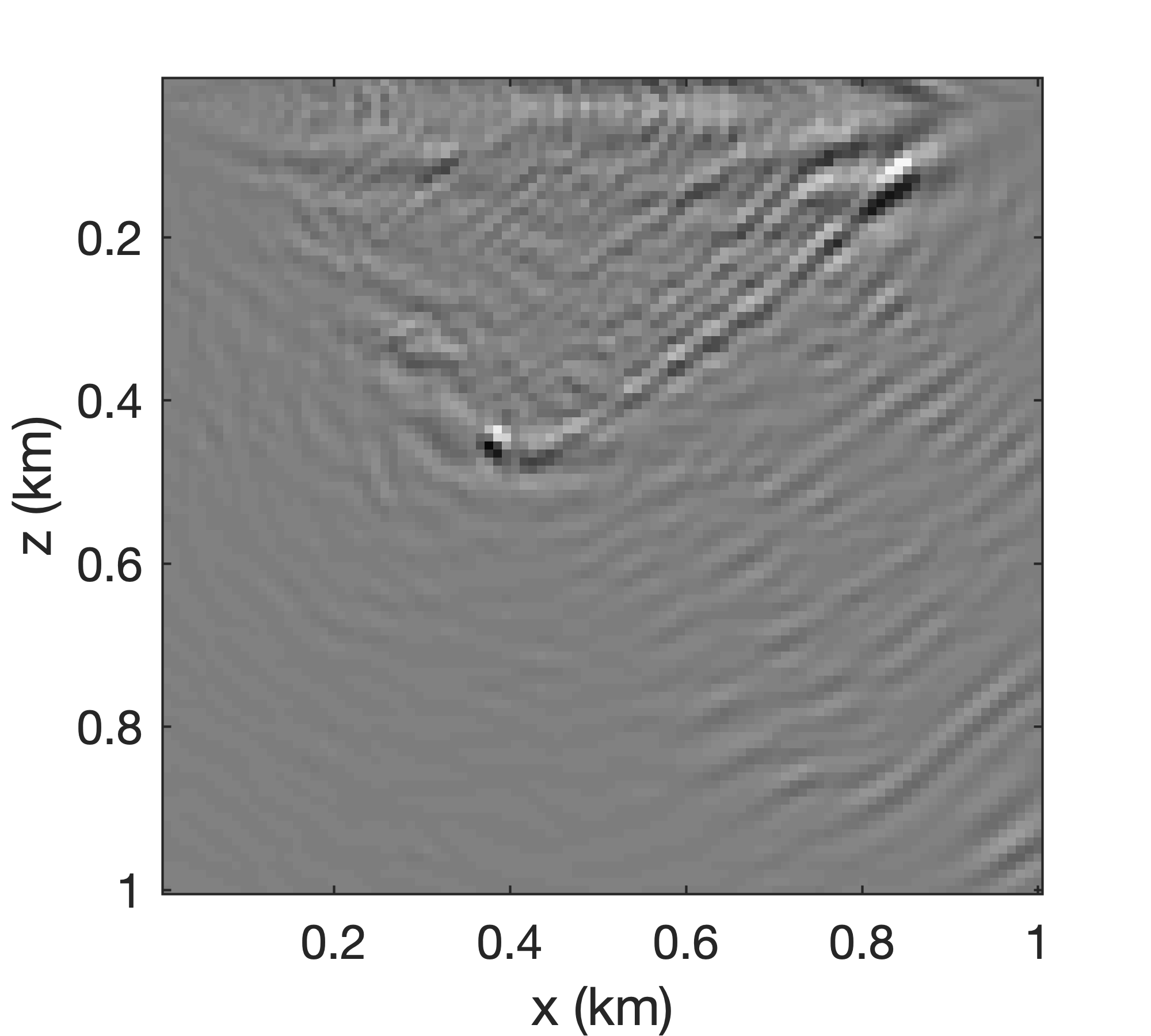
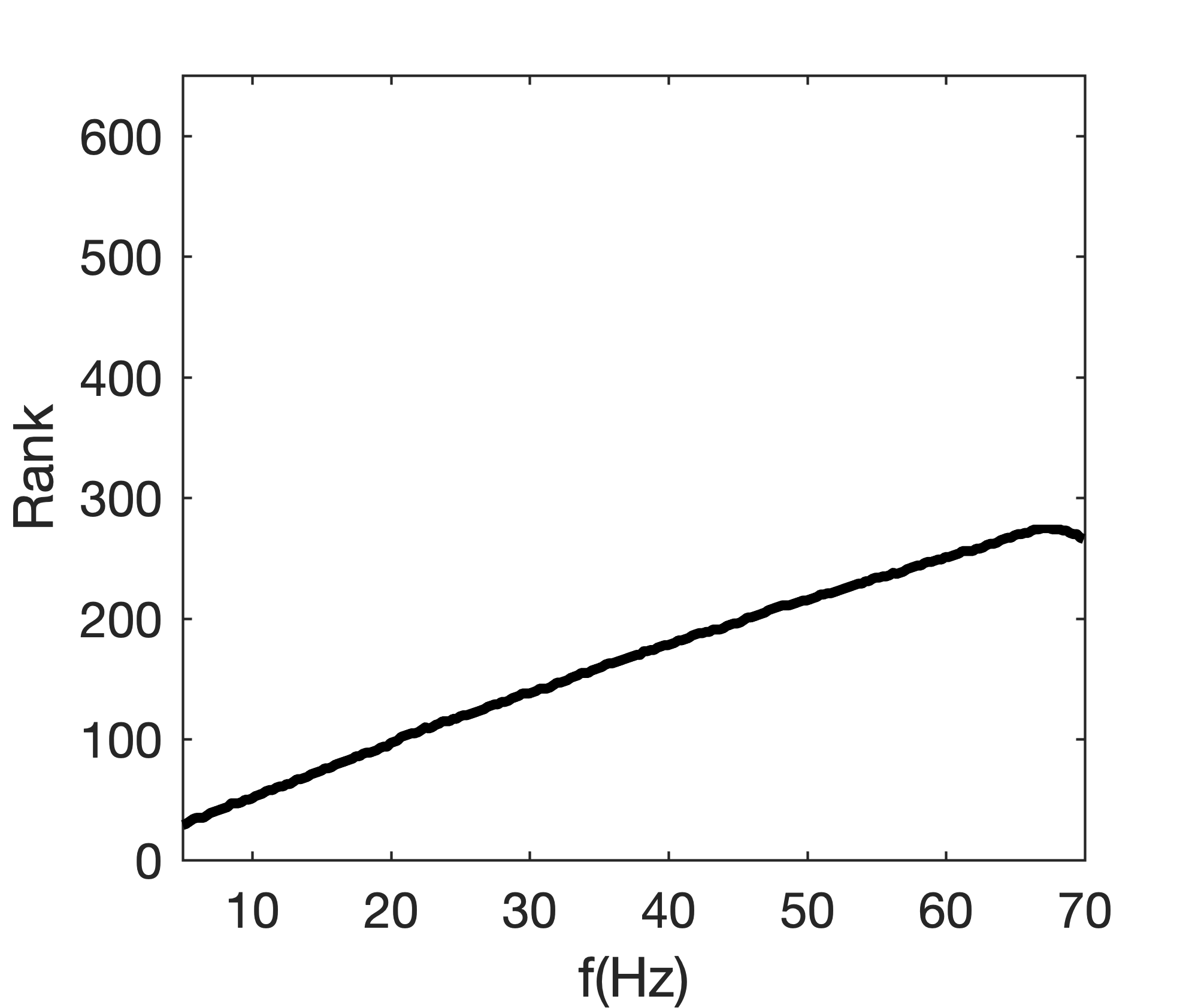
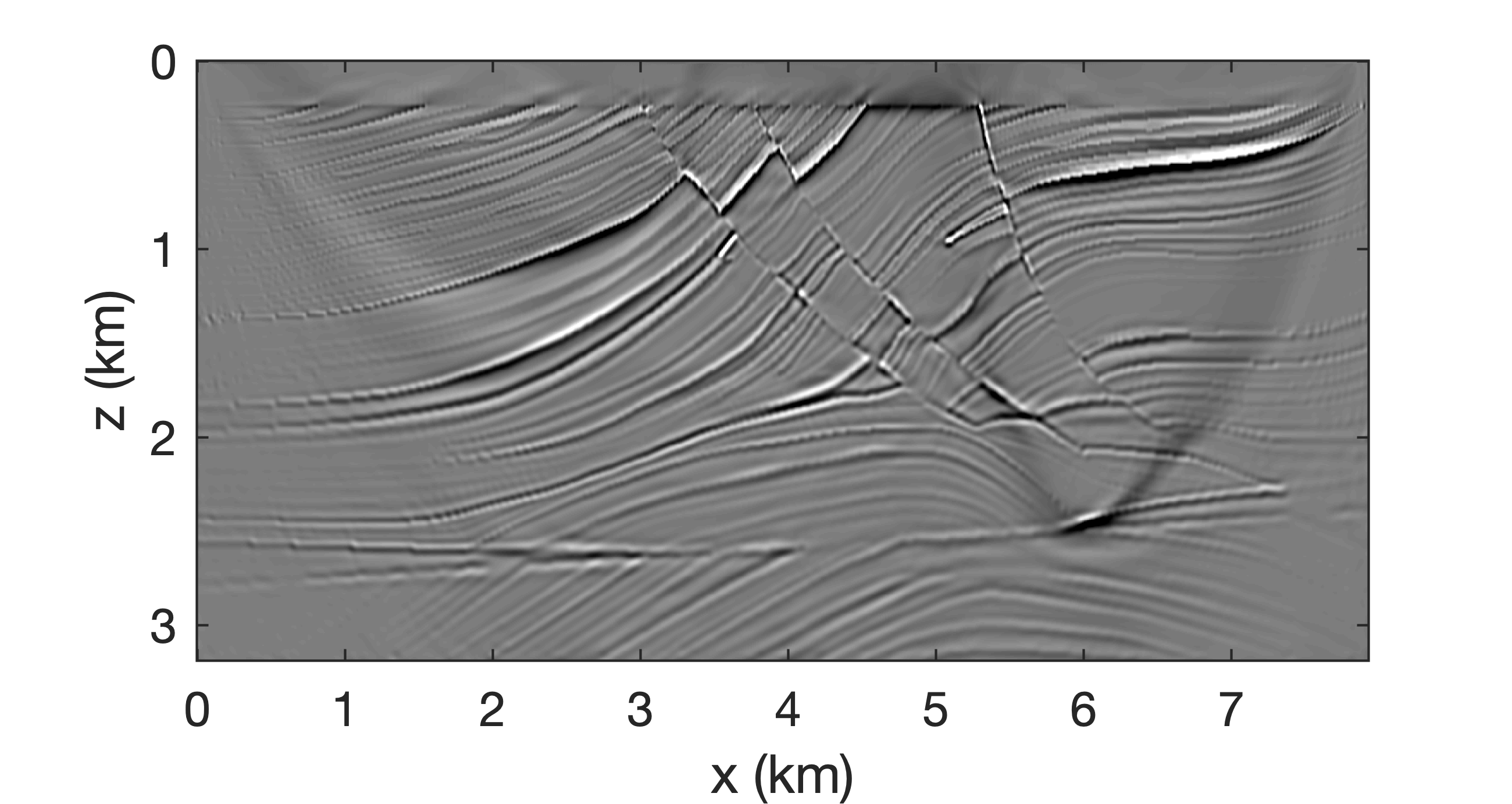
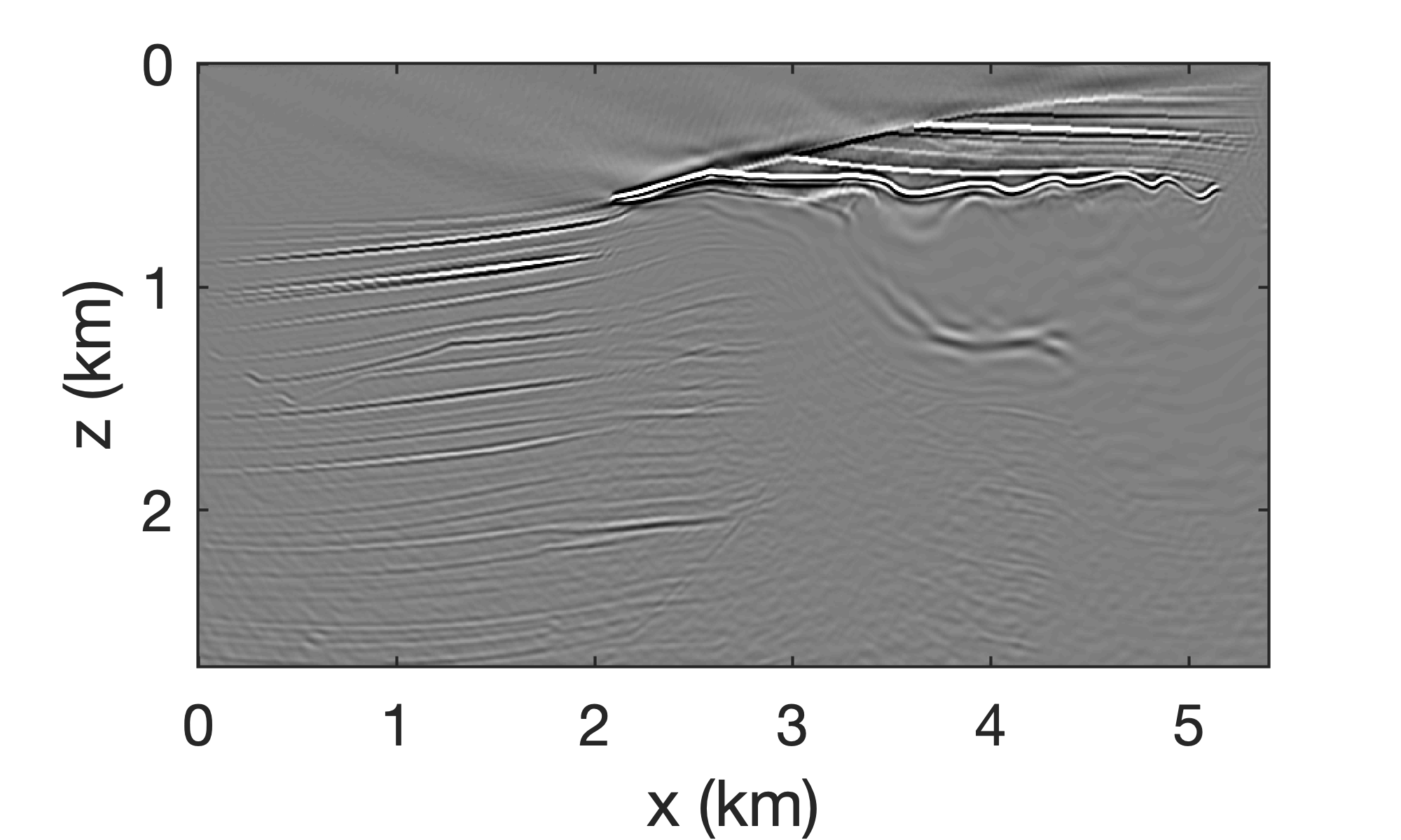
As before, we choose \(n_p\) according to the rank needed to capture \(95\%\) of the energy in the data. We plot this rank in Figure 15. Because the singular values of EIVs decay more rapidly, \(n_p=100\) is chosen, which corresponds to roughly half of the maximum rank needed to accurately represent the data at \(70\)Hz. Figure 16a contains the image obtained with a background velocity model that contains errors in the definition of top salt (Figure 14a). Compared to the image obtained with the correct background velocity model (Figure 14b), the image of Figure 14a misses key details on the salt-sediment boundary and this has a detrimental effect on the image beneath the salt. Not only is the bottom salt out of focus, so are the sediments and fault beneath the salt. By carrying out a complete new probing, factorization, and application of equation \(\ref{eq:RTM-diag}\), for the correct background velocity model, the improved result plotted in Figure 14b was obtained, which is of reasonably high quality. This shows that our factorization is capable of handling complex imaging problems in salt areas, an observation confirmed by the CIPs (cf. Figures 17a and 17b) and CIGs (cf. Figures 18a and 18b). While all slightly noisy, the images and subsurface-offset gathers behave as expected with energy focused onto the reflectors. More importantly, when we directly map the original factorization, obtained for the wrong velocities in scenario one, to the factorization for the correct velocity model using equation \(\ref{eq:factors}\) instead of recomputing the factorization after probing, the same image quality is attained for the RTM and subsurface-offset gathers. As a result, we are able to obtain the RTM image (Figure 16c), CIP (Figure 17) and CIGs (Figure 18) during scenario three with only \(4n_p\) additional wave-equation solves. For comparison, conventional RTM, without having access to EIVs, would have cost \(2n_s\) wave-equation solves; scenario two, according to Table 2 for \(q=1\), would have cost \(2n_p+4n_p+4n_p=10n_p\) solves while the direct map would have cost only \(4n_p\). Due to the chosen \(n_p=100\ll n_s=450\), we incur only a slightly higher cost compared to conducting a single migration (i.e., \(1000\) wave-equation solves versus \(900\) for conventional RTM). After the factorization, each additional RTM costs only \(400\) wave-equation solves. Moreover, factored EIVs also provide easy access to subsurface-offset gathers.


Discussion
In addition to incurring the cost of solving two wave equations per source, conventional imaging sustains substantial costs for computing subsurface-offset gathers such as CIGs (Rickett and Sava, 2002; William W Symes, 2008; Stolk et al., 2009) or angle-domain CIGs (de Bruin et al., 1990; P. Sava and Fomel, 2003; Kühl and Sacchi, 2003; Mahmoudian and Margrave, 2009; Kroode, 2012; Dafni and Symes, 2016b, 2016a). CIGs are routinely used during migration-velocity and amplitude-versus offset analysis (de Bruin et al., 1990) and in quality control during (automatic) velocity model building (W W Symes and Carazzone, 1991; Shen and Symes, 2008). The calculation of these gathers often occurs via brute force cross-correlations between the space, or sometimes, time-shifted versions of the forward and adjoint wavefields (Paul Sava and Fomel, 2006). Depending on the number of offsets and the number of CIGs, conducting these multi-dimensional cross-correlations (Paul Sava and Vasconcelos, 2011) can be as costly as calculating the wave-equation solves themselves.
Probing techniques based on the double two-way wave equation (cf. equation \(\ref{eq:two-way}\)) avoid some of these costs by computing CIPs for all subsurface offsets at the price of only two wave-equation solves and a multi-dimensional convolution with the data matrix per probing vector. While this probing technique, introduced by van Leeuwen et al. (2017), provides access to objects (e.g., CIPs) that we would normally not have access to, its complexity scales linearly with the number of CIPs, which rapidly becomes computationally infeasible. Using randomized probing techniques in combination with block Krylov iterations, we overcome this shortcoming by casting EIVs in an approximate low-rank factored form. As we have shown, this factored form allows access to conventional RTM images (cf. equation \(\ref{eq:RTM-diag}\)), various subsurface-offset gathers (Algorithms 3 and 4), and multi-scenario imaging at costs that scale with the number of factors \(n_p\). This number is typically much smaller than the number of source experiments –i.e., \(n_s\gg n_p\).
Although all of the presented examples are in 2-D, the proposed formulation is suitable to scale to 3-D for the following reasons: (1) the use of highly optimized time-domain finite-difference propagators from Devito (Luporini et al., 2018), which in addition to embracing parallelism over source experiments, supports parallelism via domain decomposition, through the Message Passing Interface (MPI)(Walker, 1992), and through multi-threading via Open Multi-Processing (OMP) (Eichenberger et al., 2013); (2) the Fourier-domain implementation of the multi-dimensional convolutions with the data matrix (see equations \(\ref{EIVprob}\) or \(\ref{EIVprob_time2}\)), which allows us to work with subsets of frequencies in parallel; and (3) the factorizations themselves, for which parallel algorithms are available (Demmel et al., 2012; Sayadi et al., 2014) to handle large problem sizes. Because we work with subsets of frequencies, we are able to limit the use of memory and computation for the factorizations. For now, we implement the probing with the regular Fourier transform, followed by subsampling, which requires storage of the full wavefield. As shown recently by Witte et al. (2019b), we do not have to store the full wavefield when using on-the-fly Fourier transforms. Since the factors are in the Fourier domain, implementing the zero-time lag imaging condition can be done via a simple summation over frequency.
In addition to the computationally feasible and manipulatable representation for EIVs, our factorization method allows for the establishment of a completely new iterative seismic imaging workflow during which
we follow the heuristic explained in the experiment section and select \(n_p\), followed by probing with random Gaussian vectors to calculate \(\mathbf{K} := [ \mathbf{E}\mathbf{W}, (\mathbf{E}\mathbf{E}^*)\mathbf{E}\mathbf{W},\cdots, (\mathbf{E}\mathbf{E}^*)^q \mathbf{E}\mathbf{W} ]\) (line 1 Algorithm 2) requiring \(6n_p\) wave-equation solves when we set \(q=1\). From \(\mathbf{K}\), we compute its QR factorization, followed by another probing with \(\mathbf{E}^*\) at \(2n_p\) wave-equation solves, in turn followed by an SVD producing the factorization \(\{\mathbf{L},\mathbf{R}\}\) with \(\mathbf{E}\approx\mathbf{L}\mathbf{R}^\ast\) for each frequency.
we have access to migrated images via equation \(\ref{eq:RTM-diag}\), to CIPs (via Algorithm 3), and (geologic dip-corrected) CIGs (via Algorithms 4) at costs that scale with \(n_p\) and that do not require additional wave-equation solves. We compute these gathers for each frequency, followed by summing over frequency to impose the zero-time lag imaging condition.
we have the option to repeat step 2 with a different background velocity model and without the need to factor the EIV again but instead, we use equation \(\ref{eq:factors-time}\) at the cost of only \(2n_p\) actions of the forward/adjoint wave equation and their inverses.
Aside from having access to different kinds of subsurface offset CIGs or angle-domain CIGs (Dafni and Symes, 2016b), this new imaging scheme has the advantage of recomputing CIGs with a different background velocity model via velocity continuation at a relatively low cost. We consider this as a highly desirable feature. For instance, this feature would allow us to recompute CIGs for quality control during velocity model building or as part of the evaluation of different background velocity model scenarios during redatuming (Kumar et al., 2019).
Subsurface-offset image gathers, which exist in various forms, are generally parameterized by horizontal subsurface offsets as in CIGs or by angles as in angle-domain CIGs (ADCIGs). In either case, the parameterization of these gathers and their recent extensions including dip-angle decompositions (Dafni and Symes, 2016b, 2016a) or micro-local parameterizations (see Kroode (2012)), does not make use of the underlying low-rank structure of EIVs. By explicitly using this low-rank structure, based on probing, factorizing, and velocity continuation, we offer an alternative formulation where the underlying linear algebra enables a natural and scalable parameterization of full-subsurface-offsete EIVs. Informed by the singular-value decay of the data and the tolerance for errors, we can make a calculated decision on the underlying rank \(n_p\). This number determines the overall computational complexity. As long as \(n_p\) is sufficiently small, our formulation can arguably compete computationally while offering unique features such as access to arbitrary subsurface-offset or angle gathers, to geologic dips, and to the option to recompute these gathers for different background velocity models at a significantly reduced cost.
The above workflow, during which we produce geologic dip-corrected CIGs, is one example of what this factored approach can offer. Other imaging schemes are possible. Since we have access to omnidirectional subsurface-offset gathers, we have the flexibility to derive filters designed to remove certain imaging artifacts as recently proposed by Dafni and Symes (2016a). Since CIPs contain the full scattering information for each point in the subsurface, we have access to the local geologic dip and to the intricacies of the wavefield interactions with the reflectors. The geologic dip corresponds to the specular dip angle of reflection introduced in recent work by Dafni and Symes (2016a).
Besides from carrying out possible filtering operations, the proposed low-rank factorization method also allows us to include recently introduced preconditioners relatively easily so that the resulting extended image volumes we produce become approximate pseudo-inverses of the extended Born modeling operator (Hou and Symes, 2015, 2017). These preconditioners remove certain imaging artifacts that may have an adverse effect on migration velocity analysis. For example, Figure 1 of a paper by Hou and Symes (2018) showed that wrong inferences can be made on the velocity because of these imaging artifacts. By including a combination of data- and image-space corrections, these imaging artifacts can be removed.
In addition to allowing for manipulations of full subsurface-offset EIVs, the proposed formulation essentially boils down to an imaging paradigm with a computational complexity that scales with the number of probing factors \(n_p\) instead of with the number of shots \(n_s\). We empirically find that the singular values of EIVs decay faster than those of monochromatic data matrices. This enables us to choose a probing size that is smaller than the number of shots \(n_s\) and arguably also smaller than a low row-rank approximation of the data matrix as proposed by Hu et al. (2009). As a result, we end up with an imaging paradigm where all imaging costs scale with the rank of the EIV factorization. In future work, we plan to select the rank adaptively per frequency, which should further enhance the performance of our low-rank factorization method.
Conclusions
Wave equation-based imaging techniques such as reverse-time migration, including the formation and manipulation of subsurface-offset gathers, are becoming more and more commonplace in modern seismic imaging workflows. While subsurface-offset image gathers carry important information on the velocity model and the local scattering mechanism, they are difficult to form and manipulate because of their high dimensionality. By combining the probing of full subsurface offset-extended image volumes via the double two-way wave equation with techniques from randomized linear algebra, we are able to cast these extended image volumes into a highly compressed and manipulatable factored form. To meet the demands of high-resolution imaging, we base the proposed low-rank factorization on probing with the time-domain wave equation and an advanced block Krylov randomized singular-value decomposition technique. The latter is designed to increase the accuracy of the factorization for high frequencies where the singular values decay more slowly. Given this factorization, we demonstrate how various subsurface image gathers can be computed without having to explicitly form the extended image volume.
While the initial cost of the factorization may exceed the cost of regular reverse-time migration, the factors provide access to gathers as a function of the omni-directional subsurface offset. These gathers allow for the computation of geologic dip-corrected common-image gathers that remain focused in situations where the reflectors are strongly dipping. Common image gathers based on a horizontal offset alone are not focused in this scenario even when the background velocity model is correct.
Because we are able to map directly the factors from one background velocity model to another without having to factorize again, the relatively high initial factorization costs are justifiable. This direct mapping of the factors is known as velocity continuation. We argue that our approach is one of the first concrete examples that show how this technique may result in a viable workflow for imaging involving salt. We demonstrate the capability of carrying out a completely new imaging experiment without having to refactorize and accomplished by using the invariance relation of extended image volumes whose applicability extends to its factored form. Since our factorization is low rank, the costs of repeated imaging experiments are small since the rank is typically much smaller than the number of shots in an imaging experiment.
Acknowledgements
All time-domain wave simulations performed in this paper are carried out with the open-source package Devito (Kukreja et al., 2016), the open source code of which is available at https://www.devitoproject.org. And this work is a collaborative effort of all the co-authors.
Appendix A - EIV’s low-rank factorization via rSVD
Due to the low-rank property of the EIV, we expect to express the monochromatic \(\mathbf{E}_i\) as the products of small or tall matrices. For instance, \(\mathbf{E}_i\) can be approximated with the singular value decomposition truncated for the \(n_p\) larger singular values of \(\mathbf{E}_i\): \[ \begin{equation} \mathbf{E}_i \approx \mathbf{\Phi}_i\mathbf{\Sigma}_i\mathbf{\Psi}^*_i, \label{LRSVD} \end{equation} \] where \(\mathbf{\Phi}_i\) and \(\mathbf{\Psi}_i\) are the \(N \times n_p\) matrices containing the \(n_p\) left and right singular vectors, respectively, associated to the \(n_p\) larger singular values listed in the \(n_p \times n_p\) diagonal matrix \(\mathbf{\Sigma}_i\). As \(n_p \ll N\), we expect to be able to store the matrices \(\mathbf{\Phi}_i\), \(\mathbf{\Psi}_i\) and the diagonal of matrix \(\mathbf{\Sigma}_i\), and extract information such as RTM or CIPs by matrix-vector multiplication successively.
In the same spirit, we may write \(\mathbf{E}\) as the product \[ \begin{equation} \mathbf{E}_i \approx \mathbf{L}_i \mathbf{R}^*_i, \label{LREIV} \end{equation} \] with \(\mathbf{L}_i\) and \(\mathbf{R}_i\) being two \(N \times n_p\) matrices, obtained from the SVD \(\eqref{LRSVD}\): \[ \begin{equation} \begin{split} \mathbf{L}_i = \mathbf{\Phi}_i \sqrt{\mathbf{\Sigma}_i}, \\ \mathbf{R}_i = \mathbf{\Psi}_i \sqrt{\mathbf{\Sigma}_i}. \end{split} \label{SVDtoLR} \end{equation} \] Note that for this monochromatic \(\mathbf{E}_i\), matrix \(\mathbf{\Sigma}_i\) is real, positive and diagonal, so the computation of its square root is implemented element-wisely on the diagonal. Once the SVD decomposition of \(\mathbf{E}_i\) performed, the construction of \(\mathbf{L}_i\) and \(\mathbf{R}_i\) is really cheap. The basic SVD method, however, has limitations in computation that involves (1) \(2n_s\) PDE solves that are extraordinarily expensive for large-scale models, and (2) the cost of SVD on the full EIV, which is of the order of \(\mathcal{O}(N^3)\) according to Holmes et al. (2007).
To circumvent the computational cost of the basic SVD, we propose using the randomized SVD-based approach (Halko et al., 2011) to obtain the low-rank representation of the full EIV. Note that we have already wrapped up the monochromatic EIV as a linear operator \(\mathbf{E}_i\) based on Helmholtz equation solves, and EIVs along frequency as a linear operator \(\mathsf{E}\) based on time-stepping solves. To keep it simple and concise, we adopt the monochromatic notations in all the low-rank recovery algorithms below and follow up with explanations of the implementation in both the frequency harmonic domain and the time-domain. The randomized SVD algorithm with the subscript neglected, is listed as Algorithm 5:
0. generate \(n_p\) random Gaussian vectors \(\mathbf{W} = [\mathbf{w}_1,\ldots,\mathbf{w}_{n_p}]\)
1. \(\mathbf{Y} = \mathbf{E}\mathbf{W}\), \(\mathbf{Y} \in \mathbb{C}^{N \times n_p}\)
2. \([\mathbf{Q},\mathbf{T}] = \text{qr}(\mathbf{Y})\),\(\mathbf{Q} \in \mathbb{C}^{N \times n_p}\), build an orthonormal basis of the range of \(\mathbf{E}\)
3. \(\mathbf{Z} = \mathbf{E}^*\mathbf{Q}, \mathbf{Z} \in \mathbb{C}^{N \times n_p}\)
4. \([\mathbf{\Phi}, \mathbf{\Sigma}, \mathbf{\Psi}] = \text{svd} (\mathbf{Z}^*)\), svd computes the top \(n_p\) singular vectors
5. set \(\mathbf{\Phi} \leftarrow \mathbf{Q}\mathbf{\Phi}\)
6. \(\mathbf{L}=\mathbf{\Phi}\sqrt{\mathbf{\Sigma}}\), \(\mathbf{R}=\mathbf{\Psi}\sqrt{\mathbf{\Sigma}}\), here \(\mathbf{L}\) and \(\mathbf{R}\) are \((N \times n_p)\) matrices
7. \(\mathbf{E} \approx \mathbf{L} \mathbf{R}^*\)
Here in line \(0\) the vector \(\mathbf{w}_{n_p}\) is one Gaussian vector. The following steps in Algorithm 5 are implemented monochromatically. Corresponding step \(0\) in the time-domain version generates tensor \(\mathsf{W}\), which is the band-limited noisy simultaneous shots located at every subsurface grid point used in the time-domain probing method. Analogously, the following steps in the time-domain version get the corresponding monochromatic tensors: \(\mathbf{Y}\), \(\mathbf{Q}\), \(\mathbf{Z}\), \(\mathbf{\Phi}\), \(\mathbf{\Psi}\), \(\mathbf{L}\) and \(\mathbf{R}\). Also the qr and svd factorizations are overloaded and implemented over all frequency slices of the corresponding tensors \(\mathbf{Y}\) and \(\mathbf{Z}^*\). Finally this algorithm combined with time-domain wave equation solver can get the recovered EIVs along all frequencies.
Baysal, E., Kosloff, D. D., and Sherwood, J. W., 1983, Reverse time migration: Geophysics, 48, 1514–1524.
Berkhout, A., 1986, Seismic inversion in terms of pre-stack migration and multiple elimination: Proceedings of the IEEE, 74, 415–427.
Biondi, B., and Symes, W. W., 2004, Angle-domain common-image gathers for migration velocity analysis by wavefield-continuation imaging: Geophysics, 69, 1283.
Biondi, B., and Tisserant, T., 2004, 3D angle-domain common-image gathers for migration velocity analysis: Geophysical Prospecting, 52, 575–591.
Castagna, J. P., and Backus, M. M., 1993, Offset-dependent reflectivity—Theory and practice of AVO analysis: Society of Exploration Geophysicists.
Castagna, J. P., Swan, H. W., and Foster, D. J., 1998, Framework for AVO gradient and intercept interpretation: Geophysics, 63, 948–956.
Claerbout, J. F., 1970, Coarse grid calculations of waves in inhomogeneous media with application to delineation of complicated seismic structure: Geophysics, 35, 407–418.
Claerbout, J. F., 1985, Imaging the earth’s interior: (Vol. 1). Blackwell scientific publications Oxford.
Crawley, S., Klochikhina, E., and Whitmore, D., 2018, A deconvolution inverse-scattering imaging condition for rTM separated wavefield imaging: In SEG technical program expanded abstracts 2018 (pp. 4372–4376). Society of Exploration Geophysicists.
Da Silva, C., and Herrmann, F. J., 2015, Optimization on the hierarchical tucker manifold - applications to tensor completion: Linear Algebra and Its Applications, 481, 131–173.
Da Silva, C., Zhang, Y., Kumar, R., and Herrmann, F. J., 2019, Applications of low-rank compressed seismic data to full waveform inversion and extended image volumes: Geophysics, 84, R371–R383.
Dafni, R., and Symes, W. W., 2016a, Kinematic artifacts in the subsurface-offset extended image and their elimination by a dip-domain specularity filter: Geophysics, 81, S477–S495.
Dafni, R., and Symes, W. W., 2016b, Scattering and dip angle decomposition based on subsurface offset extended wave-equation migration: Geophysics, 81, S119–S138.
de Bruin, C., Wapenaar, C., and Berkhout, A., 1990, Angle-dependent reflectivity by means of prestack migration: Geophysics, 55, 1223–1234.
Dell, S., and Gajewski, D., 2011, Common-reflection-surface-based workflow for diffraction imaging: Geophysics, 76, S187–S195.
Demmel, J., Grigori, L., Hoemmen, M., and Langou, J., 2012, Communication-optimal parallel and sequential qR and lU factorizations: SIAM Journal on Scientific Computing, 34, A206–A239.
Eichenberger, A. E., Mellor-Crummey, J., Schulz, M., Wong, M., Copty, N., Dietrich, R., … Lorenz, D., 2013, OMPT: An openMP tools application programming interface for performance analysis: In International workshop on openMP (pp. 171–185). Springer.
Etgen, J., Gray, S. H., and Zhang, Y., 2009, An overview of depth imaging in exploration geophysics: Geophysics, 74, WCA5–WCA17.
Halko, N., Martinsson, P.-G., and Tropp, J. A., 2011, Finding structure with randomness: Probabilistic algorithms for constructing approximate matrix decompositions: SIAM Review, 53, 217–288.
Holmes, M., Gray, A., and Isbell, C., 2007, Fast sVD for large-scale matrices: In Workshop on efficient machine learning at nIPS (Vol. 58, pp. 249–252).
Hou, J., and Symes, W. W., 2015, An approximate inverse to the extended born modeling operator: Geophysics, 80, R331–R349.
Hou, J., and Symes, W. W., 2017, An alternative formula for approximate extended born inversion: Geophysics, 82, S1–S8.
Hou, J., and Symes, W. W., 2018, Inversion velocity analysis in the subsurface-offset domain: Geophysics, 83, R189–R200.
Hu, W., Abubakar, A., and Habashy, T. M., 2009, Simultaneous multifrequency inversion of full-waveform seismic data: Geophysics, 74, R1–R14.
Kalita, M., and Alkhalifah, T., 2016, Common-image gathers using the excitation amplitude imaging condition: Geophysics, 81, S261–S269.
Kroode, F. ten, 2012, A wave-equation-based kirchhoff operator: Inverse Problems, 28, 115013.
Kukreja, N., Louboutin, M., Vieira, F., Luporini, F., Lange, M., and Gorman, G., 2016, Devito: Automated fast finite difference computation: In Domain-specific languages and high-level frameworks for high performance computing (wOLFHPC), 2016 sixth international workshop on (pp. 11–19). IEEE.
Kumar, R., Graff-Kray, M., van Leeuwen, T., and Herrmann, F. J., 2018, Low-rank representation of extended image volumes: Applications to imaging and velocity continuation: In SEG technical program expanded abstracts 2018 (pp. 4418–4422). Society of Exploration Geophysicists.
Kumar, R., Graff-Kray, M., Vasconcelos, I., and Herrmann, F. J., 2019, Target-oriented imaging using extended image volumesa low-rank factorization approach: Geophysical Prospecting, 67, 1312–1328.
Kühl, H., and Sacchi, M. D., 2003, Least-squares wave-equation migration for AVO/AVA inversion: Geophysics, 68, 262–273.
Louboutin, M., Lange, M., Luporini, F., Kukreja, N., Witte, P. A., Herrmann, F. J., … Gorman, G. J., 2018, Devito: An embedded domain-specific language for finite differences and geophysical exploration: ArXiv Preprint ArXiv:1808.01995.
Luporini, F., Lange, M., Louboutin, M., Kukreja, N., Hückelheim, J., Yount, C., … Gorman, G. J., 2018, Architecture and performance of devito, a system for automated stencil computation: CoRR, abs/1807.03032.
Mahmoudian, F., and Margrave, G. F., 2009, A review of angle domain common image gathers: CREWES Research Report, 21, 1–22.
Musco, C., and Musco, C., 2015, Randomized block Krylov methods for stronger and faster approximate singular value decomposition: In Advances in neural information processing systems (pp. 1396–1404).
Norris, M. W., Hares, M., and Wood, G., 1999, Quality control seismic data processing system:. Google Patents.
Paffenholz, J., Stefani, J., McLain, B., and Bishop, K., 2002, Sigsbee_2a synthetic subsalt dataset-image quality as function of migration algorithm and velocity model error: In 64th eAGE conference & exhibition (pp. cp–5). European Association of Geoscientists & Engineers.
Rickett, J. E., and Sava, P. C., 2002, Offset and angle-domain common image-point gathers for shot-profile migration: Geophysics, 67, 883–889.
Sava, P., and Fomel, S., 2003, Angle domain common image gathers by wavefield continuation methods: Geophysics, 68, 1065–1074.
Sava, P., and Fomel, S., 2006, Time-shift imaging condition in seismic migration: Geophysics, 71, S209–S217.
Sava, P., and Vasconcelos, I., 2011, Extended imaging conditions for wave-equation migration: Geophysical Prospecting, 59, 35–55.
Sayadi, T., Hamman, C., and Schmid, P., 2014, Parallel qR algorithm for data-driven decompositions: In Center for turbulence research, proceedings of the summer program (pp. 335–343).
Shen, P., and Symes, W. W., 2008, Automatic velocity analysis via shot profile migration: Geophysics, 73, VE49–VE59.
Stolk, C. C., Hoop, M. V. de, and Symes, W. W., 2009, Kinematics of shot-geophone migration: Geophysics, 74, WCA19–WCA34.
Symes, W. W., 2007, Reverse time migration with optimal checkpointing: Geophysics, 72, SM213–SM221.
Symes, W. W., 2008, Migration velocity analysis and waveform inversion: Geophysical Prospecting, 56, 765–790.
Symes, W. W., and Carazzone, J. J., 1991, Velocity inversion by differential semblance optimization: Geophysics, 56, 654–663.
van Leeuwen, T., and Herrmann, F. J., 2012, Wave-equation extended images: Computation and velocity continuation: EAGE annual conference proceedings.
van Leeuwen, T., Kumar, R., and Herrmann, F. J., 2017, Enabling affordable omnidirectional subsurface extended image volumes via probing: Geophysical Prospecting, 65, 385–406.
Versteeg, R., 1994, The marmousi experience: Velocity model determination on a synthetic complex data set: The Leading Edge, 13, 927–936.
Walker, D. W., 1992, Standards for message-passing in a distributed memory environment:. Oak Ridge National Lab., TN (United States).
Whitmore, N., and Crawley, S., 2012, Applications of rTM inverse scattering imaging conditions: In SEG technical program expanded abstracts 2012 (pp. 1–6). Society of Exploration Geophysicists.
Witte, P. A., Louboutin, M., Kukreja, N., Luporini, F., Lange, M., Gorman, G. J., and Herrmann, F. J., 2019a, A large-scale framework for symbolic implementations of seismic inversion algorithms in julia: Geophysics, 84, F57–F71.
Witte, P. A., Louboutin, M., Luporini, F., Gorman, G. J., and Herrmann, F. J., 2019b, Compressive least-squares migration with on-the-fly fourier transforms: Geophysics, 84, R655–R672.
Witte, P. A., Yang, M., and Herrmann, F. J., 2017, Sparsity-promoting least-squares migration with the linearized inverse scattering imaging condition: In 79th eAGE conference and exhibition 2017 (Vol. 2017, pp. 1–5). European Association of Geoscientists & Engineers.
Yang, M., Graff, M., Kumar, R., and Herrmann, F. J., 2019, Low-rank representation of subsurface extended image volumes with power iterations: In SEG technical program expanded abstracts 2019 (pp. 4470–4474). Society of Exploration Geophysicists.
We can relax this assumption by using fast Fourier-based probing methods (van Leeuwen et al., 2017).↩
In our implementation, we use Devito (https://www.devitoproject.org) for the time-domain finite difference simulations and gradient computations (Luporini et al., 2018) and JUDI (https://github.com/slimgroup/JUDI.jl) as an abstract linear algebra interface to our Algorithms (Witte et al., 2019a).↩
With some abuse of notation, we assume that the wavefields collected in the tensors are multiplied as an outer product.↩