![]()
![]()
Abstract
Nonlinear inverse problems are often hampered by non-uniqueness and local minima because of missing low frequencies and far offsets in the data, lack of access to good starting models, noise, and modeling errors. A well-known approach to counter these deficiencies is to include prior information on the unknown model, which regularizes the inverse problem. While conventional regularization methods have resulted in enormous progress in ill-posed (geophysical) inverse problems, challenges remain when the prior information consists of multiple pieces. To handle this situation, we propose an optimization framework that allows us to add multiple pieces of prior information in the form of constraints. Compared to additive regularization penalties, constraints have a number of advantages making them more suitable for inverse problems such as full-waveform inversion. The proposed framework is rigorous because it offers assurances that multiple constraints are imposed uniquely at each iteration, irrespective of the order in which they are invoked. To project onto the intersection of multiple sets uniquely, we employ Dykstra’s algorithm that scales to large problems and does not rely on trade-off parameters. In that sense, our approach differs substantially from approaches such as Tikhonov regularization, penalty methods, and gradient filtering. None of these offer assurances, which makes them less suitable to full-waveform inversion where unrealistic intermediate results effectively derail the iterative inversion process. By working with intersections of sets, we keep expensive objective and gradient calculations unaltered, separate from projections, and we also avoid trade-off parameters. These features allow for easy integration into existing code bases. In addition to more predictable behavior, working with constraints also allows for heuristics where we built up the complexity of the model gradually by relaxing the constraints. This strategy helps to avoid convergence to local minima that represent unrealistic models. We illustrate this unique feature with examples of varying complexity.
Introduction
We propose an optimization framework to include prior knowledge in the form of constraints into nonlinear inverse problems that are typically hampered by the presence of parasitic local minima. We favor this approach over more commonly known regularization via (quadratic) penalties because including constraints does not alter the objective, and therefore first- and second-order derivative information. Moreover, constraints do not need to be differentiable, and most importantly, they offer guarantees that the updated models meet the constraints at each iteration of the inversion. While we focus on seismic full-waveform inversion (FWI), our approach is more general and applies in principle to any linear or nonlinear geophysical inverse problem as long as its objective is differentiable so it can be minimized with local derivative information to calculate descent directions that reduce the objective.
In addition to the above important features, working with constraints offers several additional advantages. For instance, because models always remain within the constraint set, inversion with constraints mitigates the adverse effects of local minima which we encounter in situations where the starting model is not accurate enough or where low-frequency and long-offset data are missing or too noisy. In these situations, derivative-based methods are likely to end up in a local minimum mainly because of the oscillatory nature of the data and the non-convexity of the objective. Moreover, costs of data acquisition and limitations on available compute also often force us to work with only small subsets of data. As a result, the inversions may suffer from artifacts. Finally, noise in the data and modeling errors can also give rise to artifacts. We will demonstrate that by adding constraints, which prevent these artifacts from occurring in the estimated models, our inversion results can be greatly improved and make more geophysical and geological sense.
To deal with each of the challenging situations described above, geophysicists traditionally often rely on Tikhonov regularization, which corresponds to adding differentiable quadratic penalties that are connected to Gaussian Bayesian statistics on the prior. While these penalty methods are responsible for substantial progress in working with geophysical ill-posed and ill-conditioned problems, quadratic penalties face some significant shortcomings. Chiefly amongst these is the need to select a penalty parameter, which weights the trade-off between data misfit and prior information on the model. While there exists an extensive literature on how to choose this parameter in the case of a single penalty term (e.g., Vogel, 2002; Zhdanov, 2002; M. Sen and Roy, 2003; Farquharson and Oldenburg, 2004; Mueller and Siltanen, 2012), these approaches do not easily translate to situations where we want to add more than one type of prior information. There is also no simple prior distribution to bound pointwise values on the model without making assumptions on the underlying and often unknown statistical distribution (see Backus, 1988; Scales and Snieder, 1997; Stark, 2015). By working with constraints, we avoid making these type of assumptions.
Outline
Our primary goal is to develop a comprehensive optimization framework that allows us to directly incorporate multiple pieces of prior information in the form of multiple constraints. The main task of the optimization is to ensure that the inverted models meet all constraints during each iteration. To avoid certain ambiguities, we will do this with projections so that the updated models are unique, lie in the intersection of all constraints and remain as close as possible to the model updates provided by FWI without constraints.
There is an emerging literature on working with constrained optimization, see Lelièvre and Oldenburg (2009); Zeev et al. (2006); Bello and Raydan (2007); Baumstein (2013); Smithyman et al. (2015); Esser et al. (2015); Esser et al. (2016); Esser et al. (2018) and B. Peters and Herrmann (2017). Because this is relatively new to the geophysical community, we first start with a discussion on related work and what the limitations are of unconstrained regularization methods. Next, we discuss how to include (multiple pieces of) prior information with constraints. This discussion includes projections onto convex sets and how to project onto intersections of convex sets. After describing these important concepts, we combine them with nonlinear optimization and describe concrete algorithmic instances based on spectral-projected gradients and Dykstra’s algorithm. We conclude by demonstrating our approach on an FWI problem
Notation
Before we discuss the advantages of constrained optimization for FWI, let us first establish some mathematical notation. Our discretized unknown models live on regular grids with \(N\) grid points represented by the model vector \(\bm \in \mathbb{R}^N\), which is the result of lexicographically ordering the 2 or 3D models. In Table 1 we list a few other definitions we will use.
| description | symbol |
|---|---|
| data-misfit | \(f(\bm)\) |
| gradient w.r.t. medium parameters | \(\nabla_{\bm} f(\bm)\) |
| set (convex or non-convex) | \(\mathcal{C}\) |
| intersection of sets | \(\bigcap_{i=1}^p \mathcal{C}_i\) |
| any transform-domain operator | \(\TA \in \mathbb{C}^{M \times N}\) |
| discrete derivative matrix in 1D | \(\TD_z\) or \(\TD_x\) |
| cardinality (number of nonzero entries) or \(\ell_0\) ‘norm’ |
\(\textbf{card}(\cdot) \Leftrightarrow \| \cdot \|_0\) |
| \(\ell_1\) norm (one-norm) | \(\| \cdot \|_1\) |
Related work
A number of authors use constraints to include prior knowledge in nonlinear geophysical inverse problems. Most of these works focus on only one or maximally two constraints. For instance; Zeev et al. (2006); Bello and Raydan (2007) and Métivier and Brossier (2016) consider nonlinear geophysical problems with only bound constraints, which they solve with projection methods. Because projections implement these bounds exactly, these methods avoid complications that may arise if we attempt to approximate bound constraints by differentiable penalty functions. While standard differentiable optimization can minimize the resulting objective with quadratic penalties, there is no guarantee the inverted parameters remain within the specified range at every grid point during each iteration of the inversion. Moreover, there is also no consistent and easy way to add multiple constraints reflecting complementary aspects (e.g., bounds and smoothness) of the underlying geology. Bound constraints in a transformed-domain are discussed by Lelièvre and Oldenburg (2009).
Close in spirit to the approach we propose is recent work by Becker et al. (2015), who introduces a quasi-Newton method with projections and proximal operators (see e.g., Parikh and Boyd, 2014) to add a single \(\ell_1\) norm constraint or penalty on the model in FWI. These authors include this non-differentiable norm to induce sparsity on the model by constraining the \(\ell_1\) norm in some transformed domain or on the gradient as in total-variation minimization. While their method uses the fact that it is relatively easy to project on the \(\ell_1\)-ball, they have to work on the coefficients rather than on the physical model parameters themselves, and this makes it difficult to combine this transform-domain sparsity with say bound constraints that live in another transform-domain. As we will demonstrate, we overcome this problem by allowing for multiple constraints in multiple transform-domains simultaneously.
Several authors present algorithms that can incorporate multiple constraints simultaneously, but there are some subtle, but important algorithmic details that we discuss in this paper. For instance, the work by Baumstein (2013) employs the well-known projection-onto-convex-sets (POCS) algorithm, which can only be shown to converge to the projection of a point in special cases, see, e.g., work by Escalante and Raydan (2011) and Heinz H. Bauschke and Combettes (2011). Projecting the updated model parameters onto the intersection of multiple constraints solves this problem and offers guarantees that each model iterate (model after each iteration) remains after projection the closest in Euclidean distance to the unconstrained model and at the same time satisfies all the constraints. Different methods exist to ensure that the model iterates remain within the non-empty intersection of multiple constraint sets. Most notably, we would like to mention the work by the late Ernie Esser (Esser et al., 2018), who developed a scaled gradient projection method for this purpose involving box constraints, total-variation, and hinge-loss constraints. Esser et al. (2018) arrived at this result by using a primal-dual hybrid gradient (PDHG) method, which derives from Lagrangians associated with total-variation and hinge-loss minimization. To allow for more flexibility in the number and type of constraints, we propose the use of Dykstra’s algorithm (Dykstra, 1983; Boyle and Dykstra, 1986) instead. As we will show, this approach offers maximal flexibility in the number and complexity—i.e., we do not need closed-form expressions for the projections, of the constraints we would like to impose. We refer to Smithyman et al. (2015) and B. Peters and Herrmann (2017) for examples of successful geophysical applications of multiple constraints to FWI and its distinct advantages over adding constraints as weighted penalties.
Limitations of unconstrained regularization methods
In the introduction, we stated our requirements on a regularization framework for nonlinear inverse problems. While there are a number of successful regularization approaches such as Tikhonov regularization, a change of variables, gradient filtering and modified Gauss-Newton, these methods miss one or more of our desired properties listed in the introduction. Below we will show why the above methods do not generalize to multiple constraints or do so at the cost of introducing additional manual tuning parameters.
Tikhonov and quadratic regularization
Perhaps the most well known and widely used regularization technique in geophysics is the addition of quadratic penalties to a data-misfit function. Let us denote the model vector with medium parameters by \(\bm \in \mathbb{R}^N\) (for example velocity) where the number of grid points is \(N\). The total objective with quadratic regularization \(\phi(\bm): \mathbb{R}^N \rightarrow \mathbb{R}\) is given by \[ \begin{equation} \phi(\bm) = f(\bm) + \frac{\alpha_1}{2}\|\TR_1 \bm \|^{2}_2 + \dots + \frac{\alpha_p}{2}\|\TR_p \bm \|^{2}_2. \label{obj_qp} \end{equation} \] In this expression, the data misfit function \(f(\bm): \mathbb{R}^N \rightarrow \mathbb{R}\) measures the difference between predicted and observed data. A common choice for the data-misfit is \[ \begin{equation} f(\bm)=\frac{1}{2}\| \bd^\text{pred}(\bm) - \bd^\text{obs} \|^2_2, \label{data_misfit} \end{equation} \] where \(\bd^\text{obs}\) and \(\bd^\text{pred}(\bm)\) are observed and predicted (from the current model \(\bm\)) data, respectively. The predicted data may depend on the model parameters in a nonlinear way.
There are \(p\) regularization terms in equation \(\ref{obj_qp}\), all of which describe different pieces of prior information in the form of differentiable quadratic penalties weighted by scalar penalty parameters \(\alpha_1, \alpha_2, \dots , \alpha_p\). The operators \(R_i \in \mathbb{C}^{M_i \times N}\) are selected to penalize unwanted properties in \(\bm\)—i.e., we select each \(R\) such that the penalty terms become large if the model estimate does not lie in the desired class of models. For example, we will promote smoothness of the model estimate \(\bm\) if we add horizontal or vertical discrete derivatives as \(\TR_1\) and \(\TR_2\).
Aside from promoting certain properties on the model, adding penalty terms also changes the gradient and Hessian—i.e., we have \[ \begin{equation} \nabla_{\bm} \phi(\bm) = \nabla_{\bm}f(\bm) + \alpha_1 \TR_1^* \TR_1 \bm + \alpha_2 \TR_2^* \TR_2 \bm \label{quad_grad} \end{equation} \] and \[ \begin{equation} \nabla_{\bm}^2 \phi(\bm) = \nabla_{\bm}^2 f(\bm) + \alpha_1 \TR_1^* \TR_1 + \alpha_2 \TR_2^* \TR_2. \label{quad_hess} \end{equation} \] Both expressions, where\(^\ast\) refers to the complex conjugate transpose, contain contributions from the penalty terms designed to add certain features to the gradient and to improve the spectral properties of the Hessian by applying a shift to the eigenvalues of \(\nabla_{\bm}^2 \phi(\bm)\).
While regularization of the above type has been applied successfully, it has two important disadvantages. First, it is not straightforward to encode one’s confidence in a starting model other than including a reference model (\(\bm_\text{ref}\)) in the quadratic penalty term—i.e., \(\alpha/2 \|\bm_\text{ref} - \bm \|^2_2\) (see, e.g., Farquharson and Oldenburg (2004) and Asnaashari et al. (2013)). Unfortunately, this type of penalty tends to spread deviations with respect to this reference model evenly so we do not have easy control over its local values (cf. box constraints) unless we provide detailed prior information on the covariance. Secondly, quadratic penalties are antagonistic to models that exhibit sparse structure—i.e., models that can be well approximated by models with a small total-variation or by transform-domain coefficient (e.g. Fourier, wavelet, or curvelet) vectors with a small \(\ell_1\)-norm or cardinality (\(\|\cdot\|_0\) “norm”). Regrettably, these sparsifying norms are non-differentiable, which often leads to problems when they are added to the objective by smoothing or reweighting the norms. In either case, this can lead to slower convergence, to unpredictable behavior in nonlinear inverse problems (Amsalu Y Anagaw, 2014, p. 110; Lin and Huang, 2015, @doi:10.1190/tle36010094.1) or to a worsening of the conditioning of the Hessian (Akcelik et al., 2002). Even without smoothing non-differential penalties, there are still penalty parameters to select (Farquharson and Oldenburg, 1998; Becker et al., 2015; Lin and Huang, 2015; Xue and Zhu, 2015; Qiu et al., 2016). Finally, these issues with quadratic penalties are not purely theoretical. For instance, when working with a land dataset, (Smithyman et al., 2015) found that the above limitations of penalty terms hold in practice and found that constraint optimization overcomes these limitations, an observation motivating this work.
Gradient filtering
Aside from adding penalties to the data-misfit, we can also remove undesired model artifacts by filtering the gradients of \(f(\bm)\). When we minimize the data objective (cf. Equation \(\ref{obj_qp}\)) with standard gradient descent, this amounts to applying a filter to the gradient when we update the model—i.e., we have \[ \begin{equation} \bm^{k+1}=\bm^k - \gamma s(\nabla_{\bm}f(\bm)), \label{grad_filter} \end{equation} \] where \(\gamma\) is the step-length and \(s(\cdot)\) a nonlinear or linear filter. For instance; Brenders and Pratt (2007) apply a 2D spatial low-pass filter to prevent unwanted high-wavenumber updates to the model when inverting low-frequency seismic data. The idea behind this approach is that noise-free low-frequency data should give rise to smooth model updates. While these filters can remove unwanted high-frequency components of the gradient, this method has some serious drawbacks.
First, the gradient is no longer necessarily a gradient of the objective function (Equation \(\ref{obj_qp}\)) after applying the filter. Although the filtered gradient may under certain technical conditions remain a decent direction, optimization algorithms, such as spectral projected gradient (SPG) (Birgin et al., 1999) or quasi-Newton methods (Nocedal and Wright, 2000), expect true gradients when minimizing (constrained) objectives. Therefore gradient filtering can generally not be used in combination with these optimization algorithms, without giving up their expected behavior. Second, it is not straightforward to enforce more than one property on the model in this way. Consider, for instance, a two-filter case where \(s_1(\cdot)\) is a smoother and \(s_2(\cdot)\) enforces upper and lower bounds on the model. In this case, we face the unfortunate ambiguity \(s_2(s_1(\nabla_{\bm}f(\bm))) \neq s_1(s_2(\nabla_{\bm}f(\bm)))\). Moreover, this gradient will have non-smooth clipping artifacts if we smooth first and then apply the bounds. Amsalu Y. Anagaw and Sacchi (2017) present a method that filters the updated model instead of a gradient, but it is also not clear how to extend this filtering technique to more than one model property.
Change of variables / subspaces
Another commonly employed method to regularize nonlinear inverse problems involves certain (possibly orthogonal) transformations of the original model vector. While somewhat reminiscent of gradient filtering, this approach entails a change of variables, see, e.g., Jervis et al. (1996); Shen et al. (2005); Shen and Symes (2008) for examples in migration velocity analysis and M. Li et al. (2013); Kleinman and Berg (1992); Guitton et al. (2012); Guitton and Díaz (2012) for examples the context of waveform inversion. This approach is also known as a subspace method (Kennett and Williamson, 1988; D. W. Oldenburg et al., 1993). We can invoke this change of variables by transforming the model into \(\bp = \TT \bm\), where \(\TT\) is a (not necessarily invertible) linear operator. This changes the unconstrained optimization problem \(\min_{\bm} f(\bm)\) into another unconstrained problem \(\min_{\bp} f(\bp)\). To see why this might be helpful, we observe that the gradient becomes \(\nabla_\bp f(\bp) = \TT^* \nabla_{\bm}f(\bm)\), which shows how \(\TT\) can be designed to ‘filter’ the gradient. The matrix \(\TT\) can also represent a subspace (limited number of basis vectors such as splines, wavelets). Just as with gradient filtering, a change of variables does not easily lend itself to multiple transforms aimed at incorporating complementary pieces of prior information. However, subspace information fits directly into the constrained optimization approach if we constrain our models to be elements of the subspace. The constrained approach has the advantage that we can straightforwardly combine it with other constraints in multiple transform-domains; all constraints in the proposed framework act on the variables \(\bm\) in the physical space since we do not minimize subspace/transform-domain coefficients \(\bp\).
Modified Gauss-Newton
A more recent successful attempt to improve model estimation for certain nonlinear inverse problems concerns imposing curvelet domain \(\ell_1\)-norm based sparsity constraints on the model updates (F. Herrmann et al., 2011; Li et al., 2012, 2016). This approach converges to local minimizers of \(f(\bm)\) (and hopefully a global one) because sparsity constrained updates provably remain descent directions (Burke (1990), chapter 2; F. Herrmann et al. (2011)). However, there are no guarantees that the curvelet coefficients of the model itself will remain sparse unless the support (= locations of the non-zero coefficients) is more or less the same for each Gauss-Newton update (Li et al., 2016). L. Zhu et al. (2017) use a similar approach, but they update the transform (dictionary) at every FWI iteration.
In summary, while regularizing the gradients or model updates leads to encouraging results for some applications, the constrained optimization approach proposed in this work enforces constraints on the model estimate itself, without modifying the gradient. More importantly, while imposing constraints via projections may superficially look similar to the above methods, our proposed approach differs fundamentally in two main respects. Firstly, it projects uniquely on the intersection of arbitrarily many constraint sets — effectively removing the ambiguity of order in which constraints are applied. Secondly, it does not alter the gradients because it imposes the projections on the proposed model updates, i.e., we will project \(\bm^{k+1}=\bm^k - \nabla_{\bm}f(\bm)\) onto the constraint set.
Including prior information via constraints
Before we introduce constrained formulations of nonlinear inverse problems with multiple convex and non-convex constraint sets, we first discuss some important core properties of convex sets, of projections onto convex sets, and of projections onto intersections of convex sets. These properties provide guarantees that our approach generalizes to arbitrarily many constraint sets, i.e., one constraint set is mathematically the same as many constraint sets. The presented convex set properties also show that there is no need to somehow order of the sets to avoid ambiguity, as was the case for gradient filtering and of naive implementations of constrained optimization. The constrained formulation also stays away from penalty parameters, yet still offers guarantees all constraints are satisfied at every iteration of the inversion.
Constrained formulation
To circumvent problems related to incorporating multiple sources of possibly non-differentiable prior information, we propose techniques from constrained optimization (Boyd and Vandenberghe, 2004; Boyd et al., 2011; Parikh and Boyd, 2014; Amir Beck, 2015; Bertsekas, 2015). The key idea of this approach is to minimize the data-misfit objective while at the same time making sure that the estimated model parameters satisfy constraints. These constraints are mathematical descriptors of prior information on certain physical (e.g., maximal and minimal values for the wavespeed) and geological properties (e.g., velocity models with unconformities that lead to discontinuities in the wavespeed) on the model. We build our formulation on earlier work on constrained optimization with up to three constraint sets as presented by Lelièvre and Oldenburg (2009); Smithyman et al. (2015); Esser et al. (2015); Esser et al. (2016); Esser et al. (2018); B. Peters and Herrmann (2017).
Given an arbitrary but finite number of constraint sets (\(p\)), we formulate our constrained optimization problem as follows: \[ \begin{equation} \min_{\bm} f(\bm) \:\: \text{subject to} \:\: \bm \in \bigcap_{i=1}^p \mathcal{C}_i. \label{prob-constr} \end{equation} \] As before, \(f(\bm): \mathbb{R}^N \rightarrow \mathbb{R}\) is the data-misfit objective, which we minimize over the discretized medium parameters represented by the vector \(\bm \in \mathbb{R}^N\). Prior knowledge on this model vector resides in the indexed constraint sets \(\mathcal{C}_i, i=1 \cdots p\), each of which captures a known aspect of the Earth’s subsurface. These constraints may include bounds on permissible parameter values, desired smoothness or complexity, or limits on the number of layers in sedimentary environments and many others.
In cases where more than one piece of prior information is available, we want the model vector to satisfy these constraints simultaneously, such that we keep control over the model properties as is required for strategies that relax constraints gradually (Esser et al., 2016; B. Peters and Herrmann, 2017). Because it is difficult to think of a nontrivial example where the intersection of these sets is empty, it is safe to assume that there is at least one model that satisfies all constraints simultaneously. For instance, a homogeneous medium will satisfy many constraints, because its total-variation is zero, it has a rank of \(1\) and has parameter values between minimum and maximum values. We denote the mathematical requirement that the estimated model vector satisfies \(p\) constraints simultaneously by \(\bm \in \bigcap_{i=1}^p \mathcal{C}_i\). The symbol \(\bigcap_{i=1}^p\) indicates the intersection of \(p\) items. Before we discuss how to solve constrained nonlinear geophysical inverse problems, let us first discuss projections and examples of projections onto convex and non-convex sets.
Convex sets
A projection of \(\bm\) onto a set \(\mathcal{C}\) corresponds to solving \[ \begin{equation} \mathcal{P}_{\mathcal{C}} (\bm) = \argmin_{\bx} \frac{1}{2} \| \bx - \bm \|_2^2 \:\: \text{subject to} \:\: \bx \in \mathcal{C}. \label{proj_def} \end{equation} \] Amongst all possible model vectors \(\bx\), the above optimization problem finds the vector \(\bx\) that is closest in Euclidean distance to the input vector \(\bm\) while it lies in the constraint set. For a given model vector \(\bx\), the solution of this optimization problem depends on the constraint set \(\mathcal{C}\) and its properties. For instance, the above projection is unique for a convex \(\mathcal{C}\).
To better understand how to incorporate prior information in the form of one or more constraint sets, let us first list some important properties of constraint sets and their intersection. These properties allow us to use relatively simple algorithms to solve Problem \(\ref{prob-constr}\) by using projections of the above type. First of all, most optimization algorithms require the constraint sets to be convex. Intuitively, a set is convex if any point on the line segment connecting any two points in a set is also in the set—i.e., for all \(\bx \in \mathcal{C}\) and \(\by \in \mathcal{C}\). In that case, the following relation holds: \[ \begin{equation} c \bx +(1-c) \by \in \mathcal{C} \quad \text{for} \: 0 \leq c \leq 1. \label{cvx-set} \end{equation} \] There are a number of advantages when working with convex sets, namely
The intersection of convex sets is also a convex set. This property implies that the properties of a convex set also hold for the intersection of arbitrarily many convex sets. Practically, if an optimization algorithm is defined for a single convex set, the algorithm also works in case of arbitrarily many convex sets, as the intersection is still a single convex set.
The projection onto a convex set is unique (Boyd and Vandenberghe, 2004, sec. 8.1). When combined with property (i), this implies that the projection onto the intersection of multiple convex sets is also unique. In this context, a unique projection means that given any point outside a convex set, there exists one point in the set which is closest (in a Euclidean sense) to the given point than any other point in the set.
Projections onto convex sets are non-expansive, see e.g., (Heinz H. Bauschke and Combettes, 2011, sec. 4.1–4.2, or Dattorro (2010), E.9.3). If we define the projection operator as \(\mathcal{P}_{\mathcal{C}} (\bx)\) and take any two points \(\bx\) and \(\by\), the non-expansive property is stated as: \(\| \mathcal{P}_{\mathcal{C}} (\bx) - \mathcal{P}_{\mathcal{C}} (\by) \| \leq \| \bx - \by \|\). This property guarantees that projections of estimated models on a convex set are ‘stable’. In this context, stability implies that any pair of models moves closer or remain equally distant to each other after projection. This prevents increased separation after projection of pairs of models.
While these properties make convex sets favorites amongst practitioners of (convex) optimization, restricting ourselves to convexity is sometimes too limiting for our application. In the following sections, we may use non-convex sets in the same way as a convex set, but in that case, the above properties generally do not hold. Performance of the algorithms then needs empirical verification.
Actual projections onto a single set themselves are either available in closed-form (e.g., for bounds and certain norms) or are computed iteratively (with the alternating direction method of multipliers, ADMM, see e.g., Boyd et al. (2011) and Appendix A) when closed form-expressions for the projections are not available.
Computing projections onto intersections of convex sets
Our problem formulation, equation \(\ref{prob-constr}\), concerns multiple constraints, so we need to be able to work with multiple constraint sets simultaneously to make sure the model iterates satisfy all prior knowledge. To avoid intermediate model iterates to become physically and geologically unfeasible, we want our model iterates to satisfy a predetermined set of constraints at every iteration of the inversion process. Because of property (i) (listed above), we can treat the projection onto the intersection of multiple constraints as the projection onto a single set. This implies that we can use relatively standard (convex) optimization algorithm to solve Problem \(\ref{prob-constr}\) as long as the intersection of the different convex sets is not empty. We define the projection on the intersection of multiple sets as \[ \begin{equation} \mathcal{P_{C}}({\bm})=\operatorname*{arg\,min}_{\bx} \| \bx-\bm \|^2_2 \quad \text{s.t.} \quad \bx \in \bigcap_{i=1}^p \mathcal{C}_i. \label{def-proj} \end{equation} \] The projection of \(\bm\) onto the intersection of the sets, \(\bigcap_{i=1}^p \mathcal{C}_i\), means that we find the unique vector \(\bx\), in the intersection of all sets, that is closest to \(\bm\) in the Euclidean sense. To find this vector, we compute the projection onto this intersection via Dykstra’s alternating projection algorithm (Dykstra, 1983; Boyle and Dykstra, 1986; Heinz H Bauschke and Koch, 2015). We made this choice because this algorithm is relatively simple to implement (we only need projections on each set individually) and contains no manual tuning parameters. By virtue of property (ii), projecting onto each set separately and cyclically, Dykstra’s algorithm finds the unique projection on the intersection as long as all sets are convex (Boyle and Dykstra, 1986, Theorem 2).
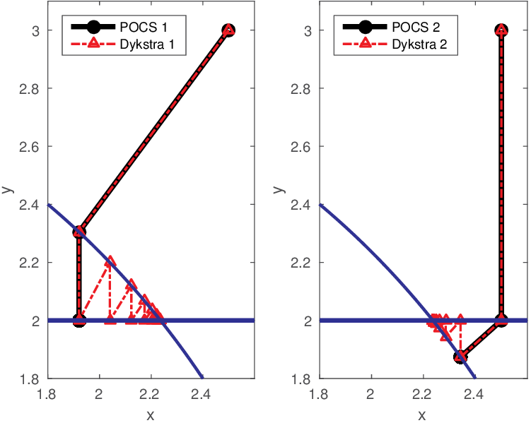
To illustrate how Dykstra’s algorithm works, let us consider the following toy example where we project the point \((2.5,\,3.0)\) onto the intersection of two constraint sets, namely a halfspace (\(\|y\|_2 \leq 2\), this corresponds to bound constraints in two dimensions) and a disk (\(x^2 + y^2 \leq 3\), this corresponds to a \(\| \cdot \|_2\)-norm ball), see Figure 1. If we are just interested in finding a feasible point in the set that is not necessarily the closest, we can use the projection onto convex sets (POCS) algorithm (also known as von Neumann’s alternating projection algorithm) whose steps are depicted by the solid black line in Figure 1. The POCS algorithm iterates \(\mathcal{P}_{\mathcal{C}_2}( \dots (\mathcal{P}_{\mathcal{C}_1}(\mathcal{P}_{\mathcal{C}_2}(\mathcal{P}_{\mathcal{C}_1}({\bm})))))\), so depending on whether we first project on the rectangle or disk, POCS finds two different feasible points. Like POCS, Dykstra projects onto each set in an alternating fashion, but unlike POCS, the solution path that is denoted by the red dashed line provably ends up at a single unique feasible point that is closest to the starting point. The solution found by Dykstra is independent of the order with which the constraints are imposed. POCS does not project onto the intersection of the two convex sets; it just solves the convex feasibility problem \[ \begin{equation} \textbf{find} \:\: \bx \in \bigcap_{i=1}^p \mathcal{C}_i \label{cvx_feasibility} \end{equation} \] instead. POCS finds a model that satisfies all constraints but which is non-unique (solution is either \((1.92,\, 2.0)\) or \((2.34,\, 1.87)\) situated at Euclidean distances \(1.16\) and \(1.14\)) and not the projection at \((2.0,\sqrt{2^2 + 3^2}\approx 2.24)\) at a minimum distance of \(1.03\). This lack of uniqueness and vicinity to the true solution of the projection problem leads to solutions that satisfy the constraints, but that may be too far away from the initial point and this may adversely affect the inversion. See also (Escalante and Raydan, 2011, Example 5.1; Dattorro, 2010, Figure 177 & Figure 182, and Heinz H. Bauschke and Combettes (2011), Figure 29.1) for further details on this important point.
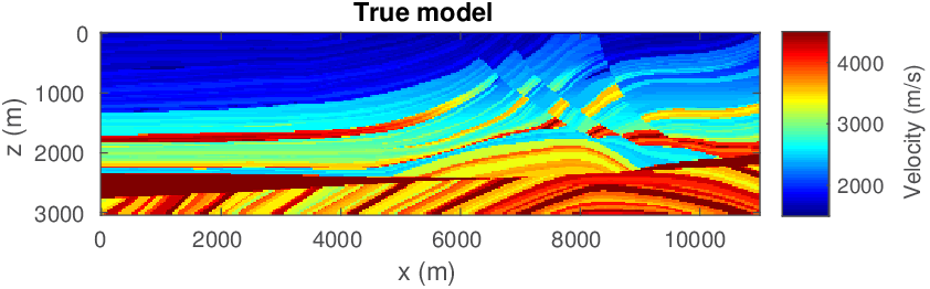
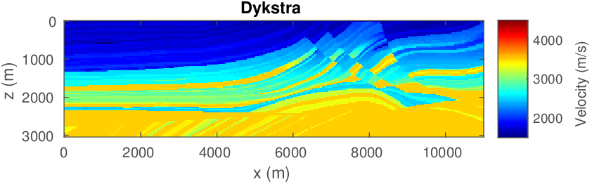
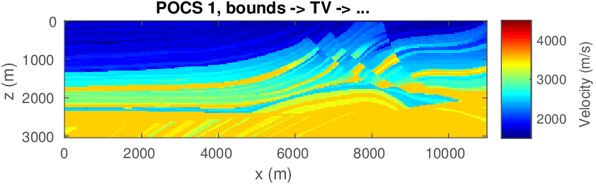
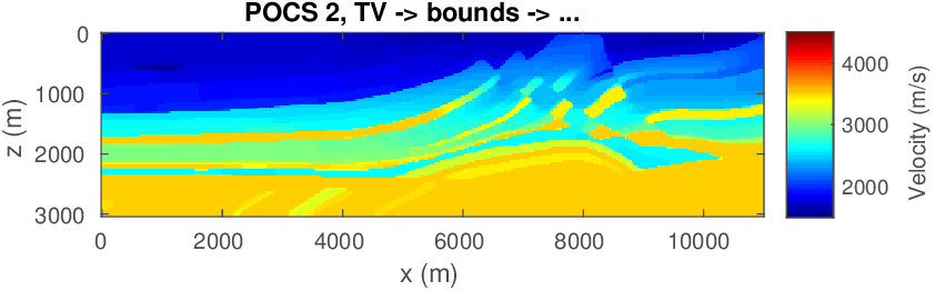
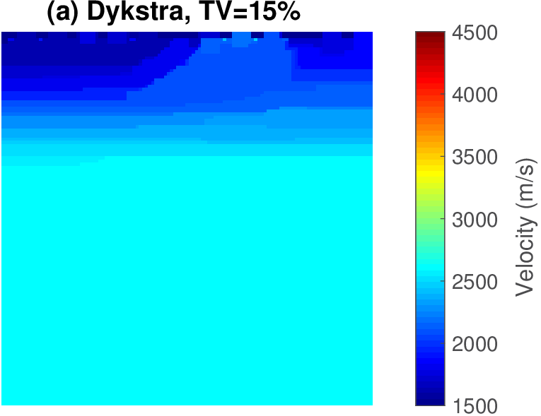
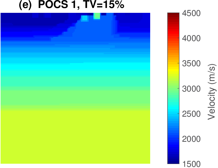
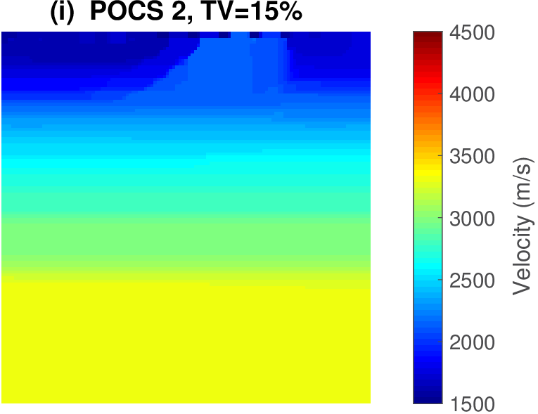
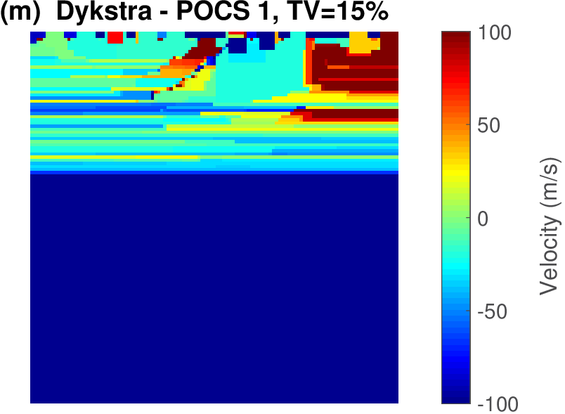
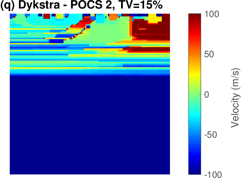
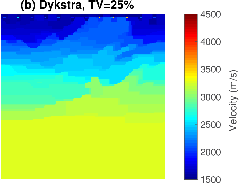
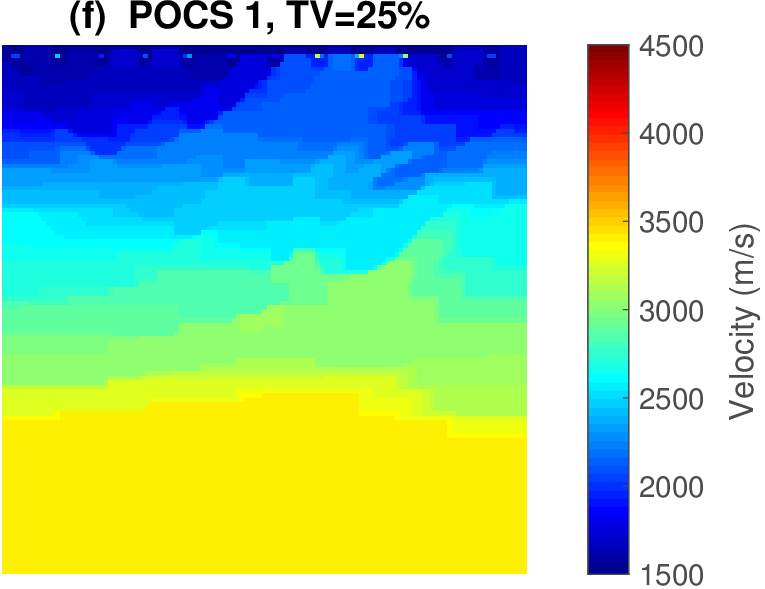
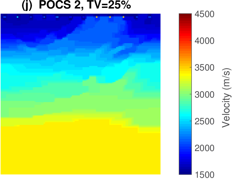
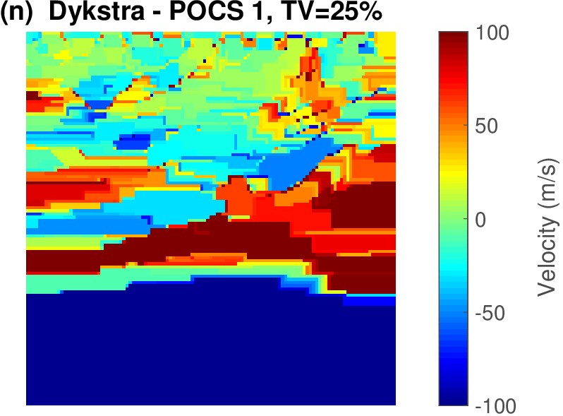
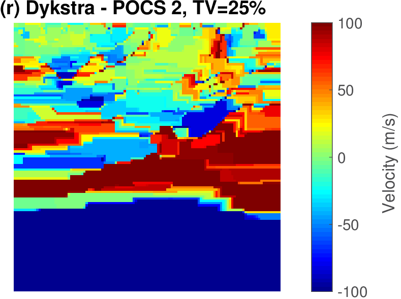
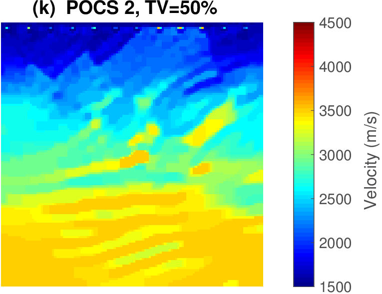
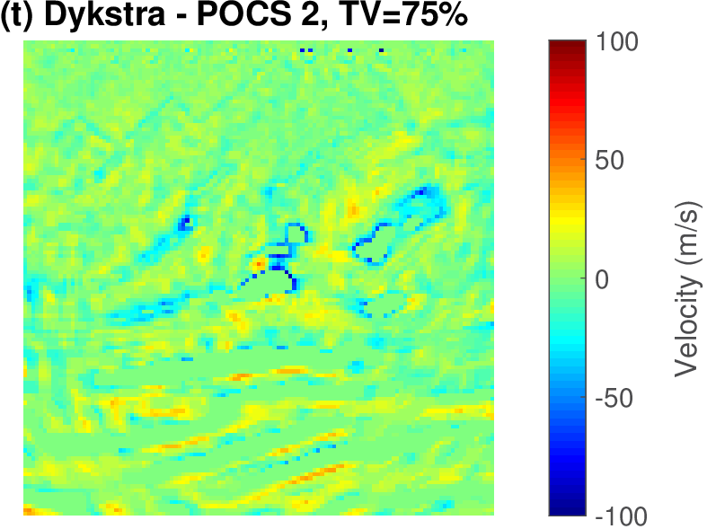
The geophysical implication of this difference between Dykstra and POCS is that the latter may end up solving a problem with unnecessarily tight constraints, moving the model too far away from the descent direction informed by the data misfit objective. We observe this phenomenon of being too constrained in Figure 1 where the two solutions from POCS are not on the boundary of both sets, but instead relatively ‘deep’ inside one of them. Aside from potential “over constraining”, the results from POCS may also differ depending which of the individual constraints is activated first leading to undesirable side effects. The issue of “over constraining” does not just occur in geometrical two-dimensional examples and it is not specific to the constraints from the previous example. Figure 2 shows what happens if we project a velocity model (with Dykstra) or find two feasible models with POCS, just as we show in Figure 1. The constraint is the intersection of bounds (\(\{ \bm \: | \: \bl_i \leq \bm_i \leq \bu_i \}\)) and total-variation (\(\{ \bm \: | \: \| \mathbf{A} \bm \|_1 \leq \sigma \}\) with scalar \(\sigma >0\) and \(A= (\TD_x^T \:\: \TD_z^T)^T\) ). While one of the POCS results is similar to the projection, the other POCS result has much smaller total-variation than the constraint enforces, i.e., the result of POCS is not the projection but a feasible point in the interior of the intersection. To avoid these issues, Dykstra is our method of choice to include two or more constraints into nonlinear inverse problems. Algorithm 1 summarizes the main steps of Dykstra’s approach, which aside from stopping conditions, is parameter free. In Figure 3 we show what happens if we replace the projection (with Dykstra’s algorithm) in projected gradient descent with POCS. Projected gradient descent solves an FWI problem with bounds and total-variation constraints while using a small number of sources and receivers and an incorrectly estimated source function. The results of Dykstra and POCS are different, while the results using POCS depend on the ordering of the sets. Dykstra’s algorithm is independent of the ordering because it finds the projection onto an intersection of convex sets, which is unique.
Algorithm \(\text{DYKSTRA}(\bm,\mathcal{P}_{\mathcal{C}_1},\mathcal{P}_{\mathcal{C}_2},\dots,\mathcal{P}_{\mathcal{C}_p})\)
0a. \(\bx_p^0=\bm\), \(k=1\) //initialize
0b. \(\by_i^0 = 0\) for \(i=1,2,\dots,p\) //initialize
WHILE stopping conditions not satisfied DO
1. \(\bx_0^k =x^{k-1}_p\)
FOR \(i=1,2,\dots,p\)
2. \(\bx^k_i = \mathcal{P}_{\mathcal{C}_i}(\bx^k_{i-1} - \by^{k-1}_i)\)
END
FOR \(i=1,2,\dots,p\)
3. \(\by^{k}_i=\bx^k_i - (\bx^k_{i-1} - \by^{k-1}_i)\)
END
4. \(k = k+1\)
END
output: \(\bx_p^k\)


Nonlinear optimization with projections
So far, we discussed a method to project models onto the intersection of multiple constraint sets. How these projections interact with nonlinear optimization problems with expensive to evaluate (data-misfit) objectives is not yet clear and also delicate given the devastating effects parasitic local minima may have on the progression of the inversion. Moreover, aside from our design criteria (multiple constraints instead of competing penalties; guarantees that model iterations remain in constraint set), we need to include a clean separation of misfit/gradient calculations and projections so that we avoid additional expensive PDE solves at all times. This separation also allows us to use different codes bases for each task (objective/gradient calculations versus projections).
Projected-gradient descent
The simplest first-order algorithm that minimizes a differentiable objective function subject to constraints is the projected gradient method (e.g., A. Beck (2014), section 9.4). This algorithm is a straightforward extension of the well-known gradient-descent method (e.g., Bertsekas, 2015, sec. 2.1) involving the following updates on the model: \[ \begin{equation} \bm^{k+1}=\mathcal{P}_{\mathcal{C}} \big(\bm^k - \gamma \nabla_{\bm}f(\bm^k)\big). \label{proj_grad_standard} \end{equation} \] A line search determines the scalar step length \(\gamma>0\). This algorithm first takes a gradient-descent step, involving an expensive gradient calculation, followed by the often much cheaper projection of the updated model back onto the intersection of the constraint sets. By construction, the computationally expensive gradient computations (and data-misfit for the line search) are separate from projections onto constraints. The projection step itself guarantees that the model estimate \(\bm^k\) satisfies all constraints at every \(k^{\text{th}}\) iteration.
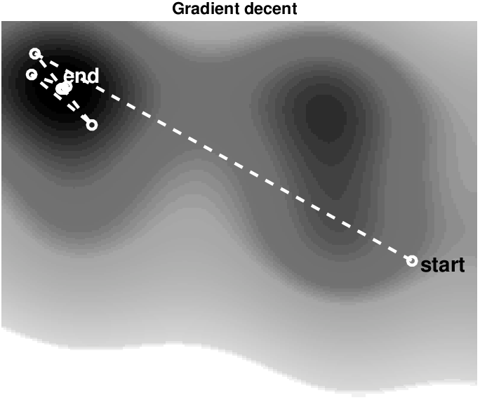
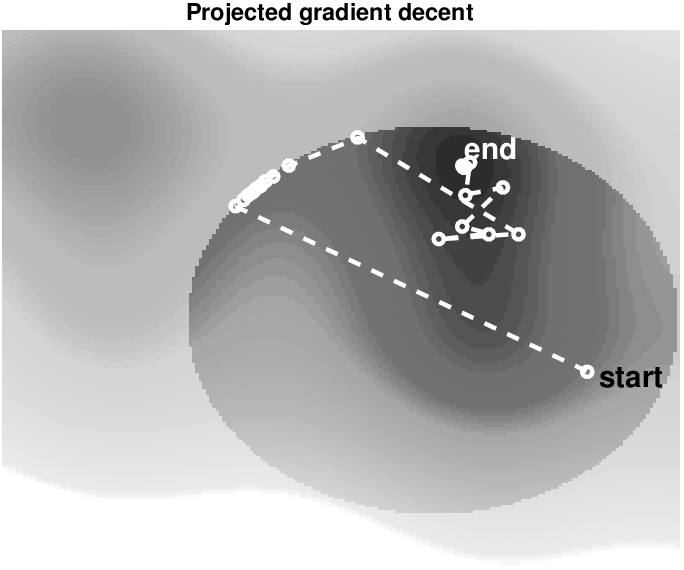
Figure 4 illustrates the difference between gradient descent to minimize a a two variable non-convex objective \(\min_\bm f(\bm)\), and projected gradient descent to minimize \(\min_\bm f(\bm) \: \text{s.t.} \: \bm \in \mathcal{C}\). If we compare the solution paths for gradient and projected gradient descent, we see that the latter explores the boundary as well as the interior of the constraint set \(\mathcal{C} = \{ \bm | \: \| \bm \|_2 \leq \sigma\}\) to find a minimizer. This toy example highlights how constraints pose upper limits (the set boundary) on certain model properties but do not force solutions to stay on the constraint set boundary. Because one of the local minima lies outside the constraint set, this example also shows that adding constraints may guide the solution to a different (correct) local minimizer. This is exactly what we want to accomplish with constraints for FWI: prevent the model estimate \(\bm^k\) to convergence to local minimizers that represent unrealistic models.
Spectral projected gradient
Standard projected gradient has two important drawbacks. First, we need to project onto the constraint set after each line search step, which involves multiple expensive objective calculations. To be more specific, we need to calculate the step-length parameter \(\gamma \in (0,1]\) if the objective of the projected model iterate is larger than the current model iterate—i.e., \(f\left(\mathcal{P}_{\mathcal{C}} (\bm^k - \gamma \nabla_{\bm}f(\bm^k))\right) > f(\bm^k)\). In that case, we need to reduce \(\gamma\) and test again whether the data-misfit is reduced. For every reduction of \(\gamma\), we need to recompute the projection and evaluate the objective, which is too expensive. Second, first-order methods do not use curvature information, which involves the Hessian of \(f(\bm)\) or access to previous gradient and model iterates. Projected gradient algorithms are therefore often slower than Newton, Gauss-Newton, or quasi-Newton algorithms for FWI without constraints.
To avoid these two drawbacks and possible complications arising from the interplay of imposing constraints and correcting for Hessians, we use the spectral projected gradient method (SPG; Birgin et al. (1999); Birgin et al. (2003)); an extension of the standard projected gradient algorithm (Equation \(\ref{proj_grad_standard}\)), which corresponds to a simple scalar scaling (related to the eigenvalues of the Hessian, see Birgin et al. (1999) and Dai and Liao (2002)). At model iterate \(k\), the SPG iterations involve the step \[ \begin{equation} \bm^{k+1}= \bm^k + \gamma \bp^k, \label{spg_upd} \end{equation} \] with update direction \[ \begin{equation} \bp^k=\mathcal{P}_{\mathcal{C}} \big( \bm^k - \alpha \nabla_{\bm}f(\bm^k) \big)-\bm^k. \label{spg_d} \end{equation} \] These two equations define the core of SPG, which differs from standard projected gradient descent in three different ways:
The spectral stepsize \(\alpha\) (Barzilai and Borwein, 1988; Raydan, 1993; Dai and Liao, 2002) is calculated by from the secant equation (Nocedal and Wright, 2000, sec. 6.1) to approximate the Hessian, leading to accelerated convergence. An interpretation of the secant equation is to mimic the action of the Hessian by scalar \(\alpha\) and use finite-difference approximations for the second derivative of \(f(\bm)\). This approach is closely related to the idea behind quasi-Newton methods. We compute \(\alpha\) as the solution of \[ \begin{equation} \TD^k = \argmin_{\TD=\alpha I} \| \TD \bs^k - \by^k \|_2, \label{BB_scaling_eq} \end{equation} \] where \(\by^k= \nabla_{\bm}f(\bm^{k+1}) - \nabla_{\bm}f(\bm^k)\) and \(\bs^k= \bm^{k+1}-\bm^k\), and \(\TI\) the identity matrix. This results in scaling by \(\alpha = {\bs_k^* \bs_k}/{\bs_k^* \by_k}\) derived from gradient and model iterates from the current and previous SPG iterations. Clearly, this is computationally cheap because \(\alpha\) is not computed by a separate line search.
Spectral-projected gradient employs non-monotone (Grippo and Sciandrone, 2002) inexact line searches to calculate the \(\gamma\) in equation \(\ref{spg_upd}\). As for all FWI problems, \(f(\bm)\) is not convex so we cannot use an exact line-search. Non-monotone means that the objective function value is allowed to increase temporarily, which often results in faster convergence and fewer line search steps, see, e.g., Birgin et al. (1999) for numerical experiments. Our intuition behind this is as follows: gradient descent iterations often exhibit a ‘zig-zag’ pattern when the objective function behaves like a ‘long valley’ in a certain direction. When the line searches are non-monotone, the objective does not always have to go down so we can take relatively larger steps along the valley in the direction of the minimizer that are slightly ‘uphill’, increasing the objective temporarily.
Each SPG iteration requires only one projection onto the intersection of constraint sets to compute the update direction (Equation \(\ref{spg_d}\)) and does not need additional projections for line search steps. This is a significant computational advantage over standard projected gradient descent, which computes one projection per line search step, see equation \(\ref{proj_grad_standard}\). From equations \(\ref{spg_upd}\) and \(\ref{spg_d}\), we observe that \(\gamma \bp^k\) lies on the line between the previous model estimate (\(\bm^k\)) and the proposed update, projected back onto the feasible set—i.e., \(\mathcal{P}_{\mathcal{C}} (\bm^k - \alpha \nabla_{\bm}f(\bm^k))\). Therefore, \(\bm^{k+1}\) is on the line segment between these two points in a convex set and the new model will satisfy all constraints simultaneously at every iteration (see equation \(\ref{cvx-set}\)). For this reason, any line search step that reduces \(\gamma\) will also be an element of the convex set. Works by Zeev et al. (2006) and Bello and Raydan (2007) confirm that SPG with non-monotone line searches can lead to significant acceleration on FWI and seismic reflection tomography problems with bound constraints compared to projected gradient descent.
In summary, each SPG iteration in Algorithm 2 requires at the \(k^\text{th}\) iteration a single evaluation of the objective \(f(\bm^k)\) and gradient \(\nabla_\bm f(\bm^k)\). In fact, SPG combines data-misfit minimization (our objective) with imposing constraints, while keeping the data-misfit/gradient and projection computations separate. When we impose the constraints, the objective and gradient do not change. Aside from computational advantages, this separation allows us to use different code bases for the objective \(f(\bm)\) and its gradient \(\nabla_\bm f(\bm)\) and the imposition of the constraints. The above separation of responsibilities also leads to a modular software design, which applies to different inverse problems that require (costly) objective and gradient calculations.
Spectral projected gradient with multiple constraints
We now arrive at our main contribution where we combine projections onto multiple constraints with nonlinear optimization with costly objective and gradient calculations using a spectral projected gradient (SPG) method. Recall from the previous section that the projection onto the intersection of convex sets in SPG is equivalent to running Dykstra’s algorithm (Algorithm 1) —i.e., we \[ \begin{equation} \begin{aligned} & \mathcal{P}_{\mathcal{C}} (\bm^k - \alpha \nabla_{\bm}f(\bm^k)) \\ & = \mathcal{P}_{\mathcal{C}_1 \bigcap \mathcal{C}_2 \bigcap \cdots \bigcap \mathcal{C}_p} (\bm^k - \alpha \nabla_{\bm}f(\bm^k)) \\ & \Leftrightarrow \text{DYKSTRA}(\bm^k - \alpha \nabla_{\bm}f(\bm^k),\mathcal{P}_{\mathcal{C}_1},\dots,\mathcal{P}_{\mathcal{C}_p}). \end{aligned} \label{proj_dyk_eq} \end{equation} \] With this equivalence established, we arrive at our version of SPG presented in Algorithm 2, which has appeared in some form in the non-geophysical literature Birgin et al. (2003) and Schmidt and Murphy (2010).
input:
// one projector per constraint set
\(\mathcal{P}_{\mathcal{C}_1}\), \(\mathcal{P}_{\mathcal{C}_2},\dots\)
\(\bm^0\) //starting model
Initialization
0. \(M = \text{integer}\), \(\eta \in (0,1)\), select initial \(\alpha\)
0. \(k=1\), select sufficient descent parameter \(\epsilon\)
WHILE stopping conditions not satisfied DO
1. \(f(\bm^k)\), \(\nabla_{\bm}f(\bm^k)\) //objective & gradient
// project onto intersection of sets:
2. \(\br^k=\text{DYKSTRA}\big( \bm^k - \alpha \nabla_{\bm}f(\bm^k),\mathcal{P}_{\mathcal{C}_1},\mathcal{P}_{\mathcal{C}_2},\dots \big)\)
3. \(\bp^k= \br^k - \bm^k\) // update direction
//save previous M objective:
4a. \(f_\text{ref} = \{f_k, f_{k-1} , \dots , f_{k-M} \}\)
4b. \(\gamma=1\)
4c. IF \(f(\bm^k+\gamma \bp^k) < \max(f_\text{ref})+ \epsilon \gamma \nabla_{\bm}f(\bm^k)^*\bp^k\)
\(\bm^{k+1} = \bm^k+\gamma\bp\) // update model iterate
\(\by_k= \nabla_{\bm}f(\bm^{k+1}) - \nabla_{\bm}f(\bm^k)\)
\(\bs_k= \bm^{k+1}-\bm^k\)
\(\alpha = \frac{\bs_k^* \bs_k}{\bs_k^* \by_k}\) // spectral steplength
\(k=k+1\)
ELSE
\(\gamma = \eta \gamma\) //step size reduction,
\(\text{go back to 4c}\)
END
output: \(\bm^k\)
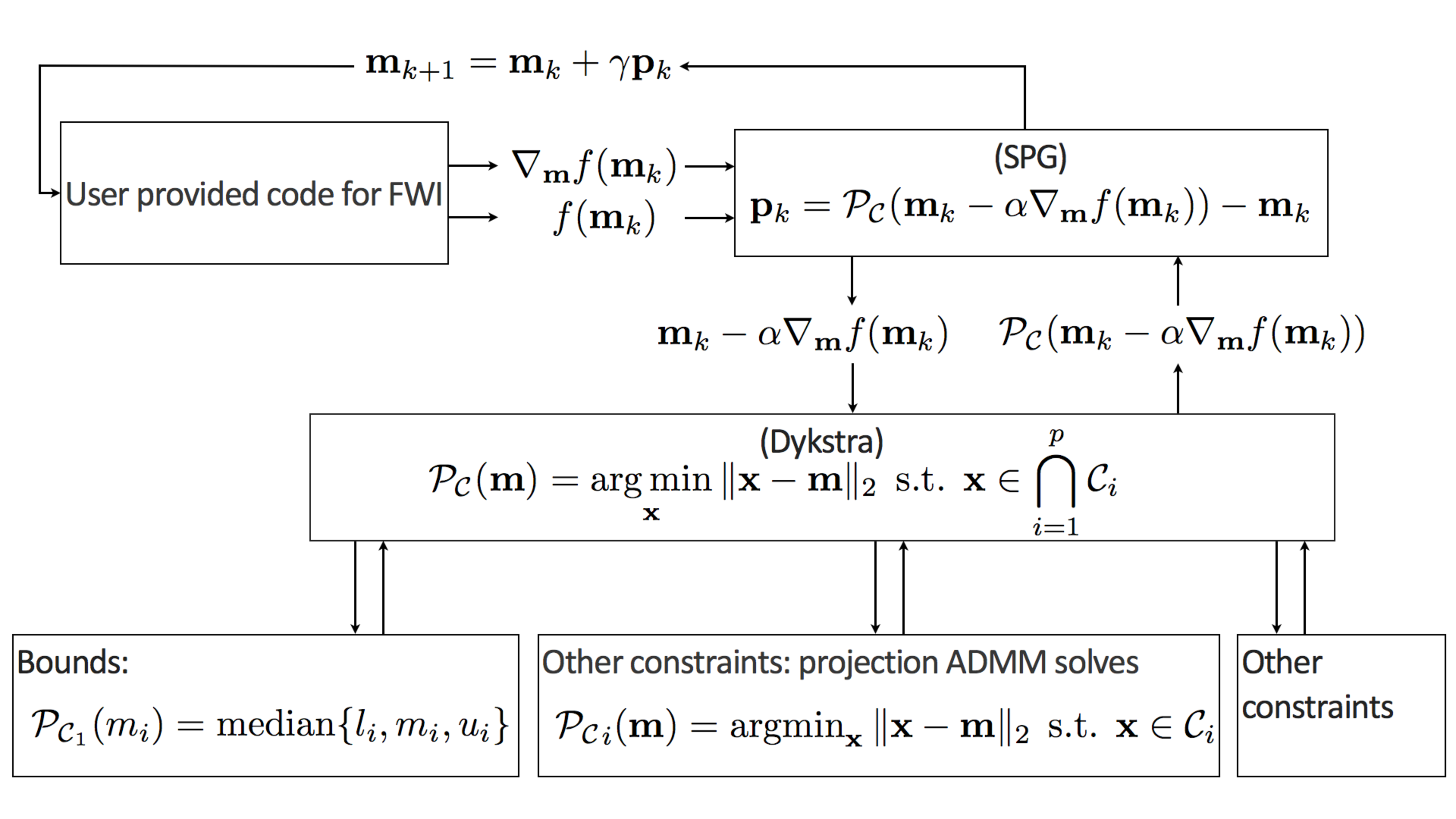
The proposed optimization algorithm for nonlinear inverse problems with multiple constraints (Eq. \(\ref{prob-constr}\)) has the following three-level nested structure:
- At the top level, we have a possibly non-convex optimization problem with a differentiable objective and multiple possibly non-differentiable constraints: \[ \begin{equation*} \min_{\bm} f(\bm) \:\: \text{subject to} \:\: \bm \in \bigcap_{i=1}^p \mathcal{C}_i, \end{equation*} \]
which we solve with the spectral projected gradient method;
At the next level, we project onto the intersection of multiple (convex) sets: \[ \begin{equation*} \mathcal{P_{C}}({\bm})=\operatorname*{arg\,min}_{\bx} \| \bx-\bm \|_2 \:\: \text{subject to} \:\: \bx \in \bigcap_{i=1}^p \mathcal{C}_i \end{equation*} \] implemented via Algorithm 1 (Dykstra’s algorithm);
At the lowest level, we project onto individual sets:
\[ \begin{equation*} \mathcal{P}_{\mathcal{C}_i}({\bm})=\operatorname*{arg\,min}_{\bx} \| \bx-\bm \|_2 \:\: \text{subject to} \:\: \bx \in \mathcal{C}_i \end{equation*} \]
for which we use ADMM (see Appendix B) if there is no closed form solution available.
While there are many choices for the algorithms at each level, we base our selection of any particular algorithm on their ability to solve each level without relying on additional manual tuning parameters. We summarized our choices in Figure 5, which illustrates the \(three\)-level nested optimization structure.
Numerical example
As we mentioned earlier, full-waveform inversion (FWI) faces problems with parasitic local minima when the starting model is not sufficiently accurate, and the data are cycle skipped. FWI also suffers when no reliable data are available at the low end of the spectrum (typically less than 3 Hertz) or at offsets larger than about two times the depth of the model. Amongst the myriad of recent, sometimes somewhat ad hoc proposals to reduce the adverse effects of these local minima, we show how the proposed constrained optimization framework allows us to include prior knowledge on the unknown model parameters with guarantees that our inverted models indeed meet these constraints for each updated model.
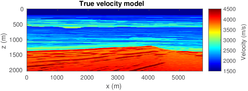
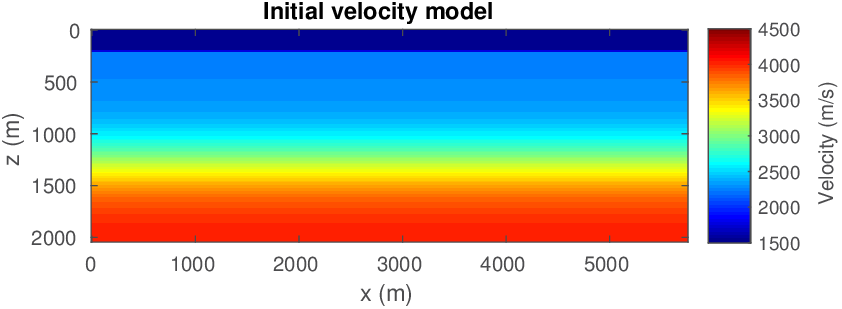
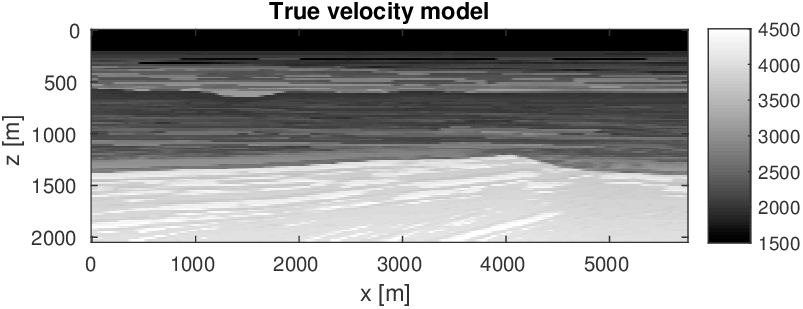
Let us consider the situation where we may not have precise prior knowledge on the actual model parameters itself, but where we may still be in a position to mathematically describe some characteristics of a good starting model. With a good starting model, we mean a model that leads to significant progress towards the true model during nonlinear inversion. So our strategy is to first improve our starting model — by constraining the inversion such that the model satisfies our expectation of what a starting model looks like — followed by a second cycle of regular FWI. We relax constraints for the second cycle to allow for model updates that further improve the data fit. Figure 6 shows the actual and initial starting models for this 2D FWI experiment. For this purpose, we take a 2D slice from the BG Compass velocity and density model. We choose this model because it contains realistic velocity “kick back”, which is known to challenge FWI. The original model is sampled at \(6\,\mathrm{m}\), and we generate “observed data” by running a time-domain (Louboutin et al., 2017) simulation code with the velocity and density models given in Figure 6. The sources and receivers (\(56\) each) are located near the surface, with \(100\,\mathrm{m}\) spacing. A coarse source and receiver spacing of a \(100\,\mathrm{m}\) amounts to about one spatial wavelength at the highest frequency in the water; well below the spatial Nyquist sampling rate.
To mimic realistic situations where the simulation kernels of the inversion miss important aspects of the wave physics, we invert for velocity only while fixing the density to be equal to one everywhere. While there are better approximations to the density model than the one we use, we intentionally use a rough approximation of the physics to show that constraints are also beneficial in that situation. To add another layer of complexity, we solve the inverse problem in the frequency domain (Da Silva and Herrmann, 2017) following the well-known multiscale frequency continuation strategy of Bunks (1995). To deal with the situation where ocean bottom marine data is often severely contaminated with noise at the low-end of the spectrum, we start the inversion on the frequency interval \(3-4\) Hertz. We define this interval as a frequency batch. We subsequently use the result of the inversion with this first frequency batch as the starting model for the next frequency batch, inverting data from the \(4-5\) Hertz interval. We repeat this process up to frequencies on the interval \(14-15\) Hertz. We also estimate the unknown frequency spectrum of the source on the fly during each iteration, using the variable projection method by (R. G. Pratt, 1999; Aravkin and Leeuwen, 2012). To avoid additional complications, we assume the sources and receivers to be omnidirectional with a flat spatial frequency spectrum.
While frequency continuation and on-the-fly source estimation are both well-established techniques by now, the combination of velocity-only inversion for a poor starting model remains challenging because we (i) ignore density variations in the inversion, which means we can never hope to fit the observed data fully; (ii) we miss the velocity kick back at roughly \(300-500\, m\) in the starting model; and (iii) we invert on an up to roughly \(10\times\) coarser grid compared to the fine \(6\, m\) grid on which the “observed” time-domain data was generated. Because of these challenges, battle-tested multiscale workflows for FWI, where we start at the low frequencies and gradually work our way up to higher frequencies, fail even if we impose bound constraints (minimum of \(1425\,(\mathrm{m}/\mathrm{s})\) and maximum \(5000\,(\mathrm{m}/\mathrm{s})\)) values for the estimated velocities) on the model. See Figure 7. Only the top \(700\,\mathrm{m}\) of the velocity model is inverted reasonably well. The bottom part, on the other hand, is far from the true model almost everywhere. The main discontinuity into the \(\geq 4000\,(\mathrm{m}/\mathrm{s})\) rock is not at the correct depth and does not have the right shape.
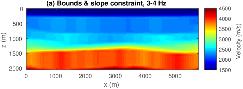
To illustrate the potential of adding more constraints on the velocity model, we follow a heuristic that combines multiple warm-started multiscale FWI cycles with relaxing the constraints. This approach was successfully employed in earlier work by Esser et al. (2016); Esser et al. (2018) and B. Peters and Herrmann (2017). Since we are dealing with a relatively undistorted sedimentary basin (see Figure 6), we impose constraints that limit lateral variations and force the inverted velocities to increase monotonically with depth during the first inversion cycle. In the second cycle, we relax this condition. We accomplish this by combining box constraints with slope constraints in the vertical direction (described in detail in Appendix B). To enforce continuity in the lateral direction, we work with tighter slope constraints in that direction. Specifically, we limit the variation of the velocity per meter in the depth direction (\(z\)-coordinate) of the discretized model \(m[i,j]=m(i\Delta z,j\Delta x)\). Mathematically, we enforce \(0 \leq (m[i+1,j]-m[i,j])/ \Delta z \leq + \infty\) for \(i=1\cdots n_z\) and \(j=1\cdots n_x\), where \(n_z\), \(n_x\) are the number of grid points in the vertical and lateral direction, and \(\Delta z\) the grid size in depth. With this slope constraint, the inverted velocities are only allowed to increase monotonically with depth, but there is no limit on how fast the velocity can increase in that direction. We impose lateral continuity by selecting the lateral slope constraint as \(-\varepsilon \leq (m[i,j+1]-m[i,j])/ \Delta x \leq +\varepsilon\quad\) for all \(i=1\cdots n_z, j=1\cdots n_x\). The scalar \(\varepsilon\) is a small number set in the physical units of velocity [meter/second] change per meter and \(\Delta x\) is the grid size in the lateral direction. We select \(\varepsilon=1.0\) for this example.
Compared to other methods that enforce continuity, e.g., via a sharpening operator in a quadratic penalty term, these slope constraints have several advantages. First, they have a natural interpretable physical parameter (\(\varepsilon\)). Second, they are met at each point in the model—i.e., they are applied and enforced pointwise; and most importantly these slope constraints do not impose more structure than needed. For instance, the vertical slope constraint only enforces monotonic increases and nothing else. We do not claim that other methods, such as Tikhonov regularization, cannot accomplish these features. We claim that we do this without nebulous parameter tuning and with guarantees that our constraints are satisfied at each iteration of FWI.
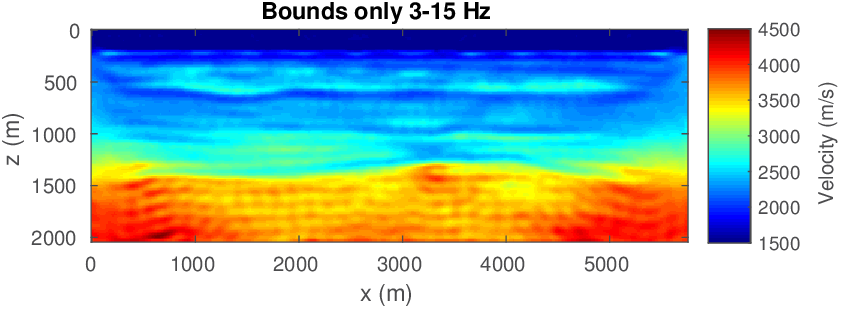
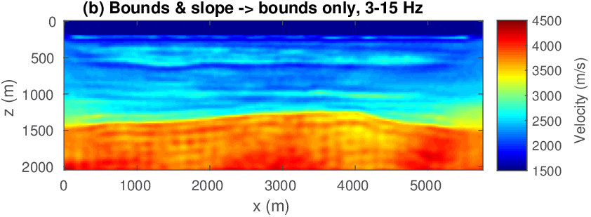
The FWI results with slope constraints for \(3-4\) Hertz data are shown in Figure 8(a). This result from the first FWI cycle improves the starting model significantly without introducing geologically unrealistic artifacts. This partially inverted model can now serve as input for the second FWI cycle where we invert data over a broader frequency range between \(3-15\) Herz (cf. Figure 8(b) ) using box constraints only. Apparently, adding slope constraints during the first cycle is enough to prevent the velocity model from moving in the wrong direction while allowing for enough freedom to get closer to the true model underlying the success of the second cycle without slope constraints. This example demonstrates that keeping the recovered velocity model after the first FWI cycle in check — via not too constrained constraints — can be a successful strategy even though final velocity model does not lie in the constraint set imposed during the first FWI cycle where velocity kick back was not allowed. We kept the computational overhead of this multi-cycle FWI method to a minimum by working with low-frequency data only during the first cycle, which reduces the size of the computational grid by a factor of about fourteen.
This example was designed to illustrate how our framework for constrained FWI can be of great practical use for FWI problems where good starting models are missing or where low-frequencies and long offsets are absent. Our proposed method is not tied to a specific constraint. For different geological settings, we can use the same approach, but with different constraints.
Discussion
Our main contribution in solving optimization problems with multiple constraints is that we employ a hierarchical divide and conquer approach to handle problems with expensive to evaluate objectives and gradients. We arrive at this result by splitting each problem into simpler and therefore computationally more manageable subproblems. We start from the top with spectral-projected gradient (SPG), which splits the constrained optimization problem into an optimality (decreasing the objective) and feasibility (satisfying all constraints) problem, and continue downwards by satisfying the individual constraints using Dykstra’s algorithm. Even at the lowest level, we employ this strategy when there is no closed form projection available for the constraints. We use the alternating direction method of multipliers (ADMM) for the examples. As a result, we end up with an algorithm that remains computationally feasible for large-scale problems with expensive to evaluate objectives and gradients.
So far, the minimization of our optimality problem relied on first-order derivative information only and what is essentially a scalar approximation of Hessian via SPG. Theoretically, we can also incorporate Dykstra’s algorithm into projected quasi-Newton (Schmidt et al., 2009) or (Gauss-) Newton methods (Schmidt et al., 2012; Lee et al., 2014). However, unlike SPG, these approaches usually require more than one projection computation per FWI iteration to solve quadratic sub-problems with constraints. We would require a more careful evaluation to see if second-order methods in this case indeed provide advantages compared to projected first-order methods such as SPG.
We also would like to note that there exist parallel versions of Dykstra and similar algorithms (Censor, 2006; Combettes and Pesquet, 2011; Heinz H Bauschke and Koch, 2015). These algorithms compute all projections in parallel, so each Dykstra iteration takes as much time as the most expensive projection computations. As a result, the time per Dykstra iteration does not necessarily increase if there are more constraint sets.
Conclusions
Because of its computational complexity and notorious local minima, full-waveform inversion easily ranks amongst one of the most challenging nonlinear inverse problems. To meet this challenge, we introduced a versatile optimization framework for (non)linear inverse problems with the following key features: (i) it invokes prior information via projections onto the intersection of multiple (convex) constraint sets and thereby avoids reliance on cumbersome trade-off parameters; (ii) it allows for imposing arbitrarily many constraints simultaneously as long as their intersection is non-empty; (iii) it projects the updated models uniquely on the intersection at every iteration and as such stays away from ambiguities related to the order in which the constraints are invoked; (iv) it guarantees that model updates satisfy all constraints simultaneously at each iteration and (v) it is built on top of existing code bases that only need to compute data-misfit objective values and gradients. These features in combination with our ability to relax and add other constraints that have appeared in the geophysical literature offer a powerful optimization framework to mitigate some of the adverse effects of local minima.
Aside from promoting certain to-be-expected model properties, our examples also confirmed that invoking multiple constraints as part of a multi-cycle inversion heuristic can lead to better results. These improvements occur as long as the constraint set is small enough to prevent adverse model updates caused by local minima to enter into the model estimate, during the first full-waveform inversion cycle(s). Provided the inversions make some progress to the solution, later inversion cycles will benefit if the tight constraints are subsequently relaxed either by dropping them or by increasing the size of the constraint set. Our examples confirm this important aspect and clearly demonstrate the advantages of working with constraints that are satisfied at each iteration of the inversion.
Compared to many other regularization methods, our approach is easily extendable to other convex or non-convex constraints. However, for non-convex constraints, we can no longer offer certain guarantees, except that all sub-problems in the alternating direction method of multipliers remain solvable without the need to tune trade-off parameters manually. We can do this because we work with projections onto the intersection of multiple sets and we split the computations into multiple pieces that have closed-form solutions.
Appendix A
Alternating Direction Method of Multipliers (ADMM) for the projection problem.
We show how to use Alternating Direction Method of Multipliers (ADMM) to solve projection problems. Iterative optimization algorithms are necessary in case there is no closed-form solution available. The basic idea is to split a ‘complicated’ problem into several ‘simple’ pieces. Consider a function that is the sum of two terms and where one of the terms contains a transform-domain operator: \(\min_{\bx} h(\bx) + g(\TA \bx)\). We proceed by renaming one of the variables, \(\TA \bx \rightarrow \bz\) and we also add the constraint \(\TA \bx=\bz\). This new problem is \(\min_{\bx,\bz} h(\bx) + g(\bz) \:\: \text{s.t.} \:\: A \bx=\bz\). The solution of both problems is the same, but algorithms to solve the new formulation are typically simpler. This formulation leads to an algorithm that can solve all projection problems discussed in this paper. Different projections only need different inputs but require no algorithmic changes.
As an example, consider the projection problem for \(\ell_1\) constraints in a transform-domain (e.g., total-variation, sparsity in the curvelet domain). The corresponding set is \(\mathcal{C} \equiv \{ \bm \: | \: \| \TA \bm \|_1 \leq \sigma \}\) and the associated projection problem is \[ \begin{equation} \mathcal{P}_{\mathcal{C}} (\bm) = \argmin_{\bx} \frac{1}{2} \| \bx - \bm \|_2^2 \quad \text{s.t} \quad \| \TA \bx \|_1 \leq \sigma. \label{proj_example_admm} \end{equation} \] ADMM solves problems with the structure: \(\min_{\bm,\bz} h(\bm) + g(\bz) \:\: \text{s.t.} \:\: \TA\bx+\mathbf{B}\bz=\bc\). The projection problem is of the same form as the ADMM problem. To see this, we use the indicator function on a set \(\mathcal{C}\) as \[ \begin{equation} \iota_{\mathcal{C}}(\bm) = \begin{cases} 0 & \text{if } \bm \in \mathcal{C},\\ +\infty & \text{if } \bm \notin \mathcal{C}.\\ \end{cases} \label{indicator} \end{equation} \] The indicator function \(\iota_{\ell_1}(\TA\bm)\) corresponds to the set \(\mathcal{C}\) that we introduced above. We use the indicator function and variable splitting to rewrite the projection problem as \[ \begin{equation} \begin{aligned} \mathcal{P}_{\mathcal{C}} (\bm)& = \argmin_{\bx} \frac{1}{2} \| \bx - \bm \|_2^2 \quad \text{s.t} \quad \| \TA \bx \|_1 \leq \sigma\\ &= \argmin_{\bx} \frac{1}{2} \| \bx - \bm \|_2^2 + \iota_{\ell_1}(\TA\bm)\\ &= \argmin_{\bx,\bz} \frac{1}{2} \| \bx - \bm \|_2^2 + \iota_{\ell_1}(\bz) \quad \text{s.t} \quad \TA\bx=\bz. \end{aligned} \label{Proj_ADMM_1} \end{equation} \] We have \(\bc=0\) and \(\mathbf{B}=-\TI\) for all projection problems in this paper. The problem stated in the last line is the sum of two functions acting on different variables with additional equality constraints. This is exactly what ADMM solves. The following derivation is mainly based on Boyd et al. (2011). Identify \(h(\bx)= \frac{1}{2} \| \bx - \bm \|_2^2\) and \(g(\bz)= \iota_{\mathcal{C}}(\bz)\). ADMM uses the augmented-Lagrangian (Nocedal and Wright, 2000, Chapter 17) to include the equality constraints \(\TA \bx - \bz = 0\) as \[ \begin{equation} L_\rho (\bx,\bz,\mathbf{v}) = h(\bx) + g(\bz) + \mathbf{v}^* (\TA\bx - \bz ) + \frac{\rho}{2} \| \TA\bx - \bz \|^2_2. \label{aug_lag_ADMM} \end{equation} \] The scalar \(\rho\) is a positive penalty parameter and \(\bv\) is the vector of Lagrangian multipliers. The derivation of the ADMM algorithm is non-trivial, see e.g., Ryu and Boyd (2016) for a derivation. Each ADMM iteration (\(k\) ) has three main steps: \[ \begin{equation} \begin{aligned} \bx^{k+1} &= \arg\min_{\bx} L_\rho (\bx,\bz^k,\mathbf{v}^k) \\ \nonumber \bz^{k+1} &= \arg\min_{\bz} L_\rho (\bx^{k+1},\bz,\mathbf{v}^k) \\ \nonumber \mathbf{v}^{k+1} &= \mathbf{v}^k + \rho (\TA \bx^{k+1} -\bz^{k+1} ). \nonumber \end{aligned} \label{Proj_ADMM_2} \end{equation} \] ADMM will converge to the solution as long as \(\rho\) is positive and reaches a stable value eventually. The choice of \(\rho\) does influence the number of iterations that are required (Nishihara et al., 2015; Xu et al., 2017, 2016) and the performance on non-convex problems (Xu et al., 2016). We use an adaptive strategy to adjust \(\rho\) at every iteration, see He et al. (2000). The derivation proceeds in the scaled form with \(\bu= \mathbf{v} / \rho\). Reorganizing the equations leads to \[ \begin{equation} \begin{aligned} \bx^{k+1} &= \arg\min_{\bx} \Big(h(\bx) + \frac{\rho}{2} \| \TA \bx - \bz^{k} + \bu^k \|^2_2 \Big) \\ \nonumber \bz^{k+1} &= \arg\min_{\bz} \Big(g(\bz) + \frac{\rho}{2} \| \TA \bx^{k+1} - \bz + \bu^k \|^2_2 \Big) \\ \nonumber \bu^{k+1} &= \bu^k + \TA \mathbf{x}^{k+1} - \bz^{k+1}. \nonumber \end{aligned} \label{Proj_ADMM_3} \end{equation} \] Now insert the expressions for \(h(\bx)\) and \(g(\bz)\) to obtain the more explicitly defined iterations \[ \begin{equation} \begin{aligned} \bx^{k+1} &= \arg\min_{\bx} \bigg(\frac{1}{2} \| \bx - \bm \|_2^2 + \frac{\rho}{2} \| \TA \bx - \bz^{k} + \bu^k \|^2_2 \bigg) \\ \nonumber \bz^{k+1} &= \arg\min_{\bz} \Big(\iota_{\mathcal{C}}(\bz) + \frac{\rho}{2} \| \TA \bx^{k+1} - \bz + \bu^k \|^2_2 \Big) \\ \nonumber \bu^{k+1} &= \bu^k + \TA \bx^{k+1} - \bz^{k+1}. \nonumber \end{aligned} \label{Proj_ADMM_4} \end{equation} \] If we replace the minimization steps with their respective close-form solutions, we have the following pseudo-algorithm: \[ \begin{equation} \begin{aligned} \bx^{k+1} &= (\rho \TA^*\TA + I)^{-1} \big( \rho \TA^*( \bz^k - \bu^k)+\bm \big)\\ \nonumber \bz^{k+1} &= \mathcal{P}_\mathcal{C}(\TA \bx^{k+1} + \bu^k ) \\ \nonumber \bu^{k+1} &= \bu^k + \TA \bx^{k+1} - \bz^{k+1}. \nonumber \end{aligned} \label{Proj_ADMM_5} \end{equation} \] This shows that the second minimization step in the ADMM algorithm to compute a projection is a different projection. The projection part of ADMM for the transform-domain \(\ell_1\) constraint (\(\bz^{k+1} = \mathcal{P}_\mathcal{C}(\TA \bx^{k+1} + \bu^k ) = \arg\min_\bz 1/2 \| \bz - \bv \|^2_2 \:\: \text{s.t} \:\: \| \bz\|_1 \leq \sigma\), with \(\bv = \TA \bx^{k+1} + \bu^k \)) is a much simpler problem than the original projection problem (Equation \(\ref{proj_example_admm}\)) because we do not have the transform-domain operator multiplied with the optimization variable. The \(\bx\)-minimization step is equivalent to the least-squares problem \[ \begin{equation} \begin{split} \bx^{k+1} = \argmin_{\bx} \bigg\| \begin{pmatrix} \sqrt{\rho}\TA \\ \TI \end{pmatrix} \bx -\begin{pmatrix} \sqrt{\rho}(\bz^k-\bu^k) \\ \bm \end{pmatrix} \bigg\|_2 \end{split} \label{ADMM_x_sub} \end{equation} \] We can solve the \(\bx\)-minimization problem using direct (QR-factorization) or iterative methods (LSQR (Paige and Saunders, 1982) on the least-squares problem or conjugate-gradient on the normal equations). We adjust the penalty parameter \(\rho\) every ADMM cycle. We recommend iterative algorithms for this situation, to avoid recomputing the QR factorization every ADMM iteration. Iterative methods allow for the current estimate of \(\bx\) as the initial guess. Moreover, \(\bz\) and \(\bu\) change less as the ADMM iterations progress, meaning that the previous \(\bx\) is a better and better initial guess. Therefore, the number of LSQR iterations typically decreases as the number of ADMM iterations increases. Algorithm 3 shows the ADMM algorithm to compute projections, including automatic adaptive penalty parameter adjustment. For numerical experiments in this paper, we use \(\mu = 10\), \(\tau = 2\) as suggested by Boyd et al. (2011).
\(\textbf{input:}\) \(\bm\), transform-domain \(\TA\),
norm/bound/cardinality projector \(\mathcal{P}_\mathcal{C}\)
\(x_0=\bm\), \(\bz_0=0\), \(\bu_0=0\), \(k=1\),
select \(\tau>1\), \(\mu>1\)
WHILE not converged
\(\bx^{k+1} = (\rho \TA^*\TA + \TI)^{-1} \big( \rho \TA^*( \bz^k - \bu^k)+\bm \big)\)
\(\bz^{k+1} = \mathcal{P}_\mathcal{C}(\TA \bx^{k+1} + \bu^k )\)
\(\bu^{k+1} = \bu^k + \TA \mathbf{x}^{k+1} - \bz^{k+1}\)
\(\br = \TA \bx^{k+1}- \bz^{k+1} \)
\(\bs = \rho \TA^* (\bz^{k+1} - \bz^{k})\)
IF \(\|\br\| > \mu \| \bs \|\) //increase penalty
\(\rho = \rho \tau\)
\(\bu = \bu / \tau\)
IF \(\| \bs \| > \mu \|\br\|\) //decrease penalty
\(\rho = \rho / \tau\)
\(\bu = \bu \tau\)
ELSE
\(\rho\) //do nothing
END
END
\(\textbf{output:}\) \(\bx\)
If we have a different constraint set, but same transform domain operator, we only change the projector that we pass to ADMM. If the constraint set is the same, but the transform-domain operator is different, we provide a different \(\TA\) to ADMM. Therefore, the various types of transform-domain \(\ell_1\), cardinality or bound constraints all use ADMM to compute the projection, but with (partially) different inputs.
Appendix B
Transform-domain bounds / slope constraints
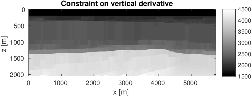
Our main interest in transform-domain bound constraints originates from the special case of slope constraints, see e.g., Petersson and Sigmund (1998) and Heinz H Bauschke and Koch (2015) for examples from computational design. Lelièvre and Oldenburg (2009) propose a transform-domain bound constraint in a geophysical context, but use interior point algorithms for implementation. In our context, slope means the model parameter variation per distance unit, over a predefined path in the model. For example, the slope of the 2D model parameters in the vertical direction (z-direction) form the constraint set \[ \begin{equation} \mathcal{C} \equiv \{ \bm \: | \: \bb^l_j \leq ( (\TD_z \otimes \TI_x) \bm)_j \leq \bb^u_j \}, \label{slope_const} \end{equation} \] with Kronecker product \(\otimes\), identity matrix with dimension equal to the x-direction \(\TI_x\), and \(\TD_z\) is a 1D finite-difference matrix corresponding to the z-direction. \(\bb_j^l\) is element \(j\) of the lower bound vector. An appealing property of this constraint is the physical meaning in a pointwise sense. If the model parameters are acoustic velocity in meters per second and the grid is also in units of meters, the constraint then defines the maximum velocity increment/decrement per meter in a direction. This type of direct physical meaning of a constraint is not available for \(\ell_1\), rank or Nuclear norm constraints; those constraints assign a single scalar value to a property of the entire model.
There are different modes of operation of the slope constraint:
Approximate monotonicity. The acoustic velocity generally increases with depth inside the Earth. This means the parameter values increase (approximately) monotonically with dept (positivity of the vertical discrete gradient). The set \(\mathcal{C} \equiv \{ \bm \: | \: -\varepsilon \leq ((\TD_z \otimes \TI_x) \bm)_j \leq +\infty \}\) describes this situation, where \(\varepsilon > 0\) is a small number. Exact monotonicity corresponds to \(\varepsilon = 0\), which means we allow the model parameter values to increase arbitrarily fast with increasing depth, but enforce a slow decrease of parameter values when looking into the depth direction.
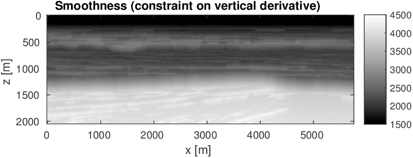
Smoothness. We obtain a type of smoothness by setting both bounds to small numbers: \(\mathcal{C} \equiv \{ \bm \: | \: -\varepsilon_1 \leq ((\TD_z \otimes \TI_x) \bm)_j \leq +\varepsilon_2 \}\), where \(\varepsilon_1 > 0\), \(\varepsilon_2 > 0\) are small numbers. This type of smoothness results in a different projection problem than if smoothness is obtained using constraints based on norms or subspaces. Another difference is that the slope constraint is inherently locally defined.
The slope constraint may be defined along any path using any discrete derivative matrix. Higher order derivatives lead to bounds on different properties. Approximate monotonicity of parameter values can also be obtained using other constraints. Esser et al. (2016) use the norm based hinge-loss constraint. However, we prefer to work with linear inequalities because norm based constraints are not defined pointwise and do not have the direct physical interpretation as described above. Figure 9 shows what happens when we project a velocity model onto the different slope constraint sets.
Akcelik, V., Biros, G., and Ghattas, O., 2002, Parallel multiscale gauss-newton-krylov methods for inverse wave propagation: In Supercomputing, aCM/IEEE 2002 conference (pp. 41–41). doi:10.1109/SC.2002.10002
Anagaw, A. Y., 2014, Full waveform inversion using simultaneous encoded sources based on first-and second-order optimization methods: PhD thesis,. University of Alberta.
Anagaw, A. Y., and Sacchi, M. D., 2017, Edge-preserving smoothing for simultaneous-source fWI model updates in high-contrast velocity models: GEOPHYSICS, 0, 1–18. doi:10.1190/geo2017-0563.1
Aravkin, A. Y., and Leeuwen, T. van, 2012, Estimating nuisance parameters in inverse problems: Inverse Problems, 28, 115016.
Asnaashari, A., Brossier, R., Garambois, S., Audebert, F., Thore, P., and Virieux, J., 2013, Regularized seismic full waveform inversion with prior model information: GEOPHYSICS, 78, R25–R36. doi:10.1190/geo2012-0104.1
Backus, G. E., 1988, Comparing hard and soft prior bounds in geophysical inverse problems: Geophysical Journal International, 94, 249. doi:10.1111/j.1365-246X.1988.tb05899.x
Barzilai, J., and Borwein, J. M., 1988, Two-point step size gradient methods: IMA Journal of Numerical Analysis, 8, 141–148. doi:10.1093/imanum/8.1.141
Baumstein, A., 2013, POCS-based geophysical constraints in multi-parameter full wavefield inversion: 75th eAGE conference and exhibition 2013. EAGE.
Bauschke, H. H., and Combettes, P. L., 2011, Convex analysis and monotone operator theory in hilbert spaces: (1st ed.). Springer Publishing Company, Incorporated.
Bauschke, H. H., and Koch, V. R., 2015, Projection methods: Swiss army knives for solving feasibility and best approximation problems with halfspaces: Contemporary Mathematics, 636, 1–40.
Beck, A., 2014, Introduction to nonlinear optimization: Society for Industrial; Applied Mathematics. doi:10.1137/1.9781611973655
Beck, A., 2015, On the convergence of alternating minimization for convex programming with applications to iteratively reweighted least squares and decomposition schemes: SIAM Journal on Optimization, 25, 185–209. doi:10.1137/13094829X
Becker, S., Horesh, L., Aravkin, A., Berg, E. van den, and Zhuk, S., 2015, General optimization framework for robust and regularized 3D fWI: In 77th eAGE conference and exhibition 2015.
Bello, L., and Raydan, M., 2007, Convex constrained optimization for the seismic reflection tomography problem: Journal of Applied Geophysics, 62, 158–166. doi:http://dx.doi.org/10.1016/j.jappgeo.2006.10.004
Bertsekas, D. P., 2015, Convex optimization algorithms: Athena Scientific.
Birgin, E. G., and Raydan, M., 2005, Robust stopping criteria for dykstra’s algorithm: SIAM Journal on Scientific Computing, 26, 1405–1414. doi:10.1137/03060062X
Birgin, E. G., Martínez, J. M., and Raydan, M., 1999, Nonmonotone spectral projected gradient methods on convex sets: SIAM J. on Optimization, 10, 1196–1211. doi:10.1137/S1052623497330963
Birgin, E. G., Martínez, J. M., and Raydan, M., 2003, Inexact spectral projected gradient methods on convex sets: IMA Journal of Numerical Analysis, 23, 539. doi:10.1093/imanum/23.4.539
Boyd, S., and Vandenberghe, L., 2004, Convex optimization: Cambridge University Press.
Boyd, S., Parikh, N., Chu, E., Peleato, B., and Eckstein, J., 2011, Distributed optimization and statistical learning via the alternating direction method of multipliers: Found. Trends Mach. Learn., 3, 1–122. doi:10.1561/2200000016
Boyle, J. P., and Dykstra, R. L., 1986, A method for finding projections onto the intersection of convex sets in hilbert spaces: In Advances in order restricted statistical inference: Proceedings of the symposium on order restricted statistical inference held in iowa city, iowa, september 11–13, 1985 (pp. 28–47). Springer New York. doi:10.1007/978-1-4613-9940-7_3
Brenders, A. J., and Pratt, R. G., 2007, Full waveform tomography for lithospheric imaging: Results from a blind test in a realistic crustal model: Geophysical Journal International, 168, 133–151. doi:10.1111/j.1365-246X.2006.03156.x
Bunks, C., 1995, Multiscale seismic waveform inversion: Geophysics, 60, 1457. doi:10.1190/1.1443880
Burke, J., 1990, Basic convergence theory:. University of Washington.
Censor, Y., 2006, Computational acceleration of projection algorithms for the linear best approximation problem: Linear Algebra and Its Applications, 416, 111–123. doi:http://dx.doi.org/10.1016/j.laa.2005.10.006
Combettes, P. L., and Pesquet, J.-C., 2011, Proximal splitting methods in signal processing: In H. H. Bauschke, R. S. Burachik, P. L. Combettes, V. Elser, D. R. Luke, & H. Wolkowicz (Eds.), Fixed-point algorithms for inverse problems in science and engineering (Vol. 49, pp. 185–212). Springer New York. doi:10.1007/978-1-4419-9569-8_10
Da Silva, C., and Herrmann, F. J., 2017, A Unified 2D/3D Large Scale Software Environment for Nonlinear Inverse Problems: ArXiv E-Prints.
Dai, Y., and Liao, L., 2002, R‐linear convergence of the barzilai and borwein gradient method: IMA Journal of Numerical Analysis, 22, 1. doi:10.1093/imanum/22.1.1
Dattorro, J., 2010, Convex optimization & euclidean distance geometry: Meboo Publishing USA.
Dykstra, R. L., 1983, An algorithm for restricted least squares regression: Journal of the American Statistical Association, 78, 837–842. doi:10.1080/01621459.1983.10477029
Escalante, R., and Raydan, M., 2011, Alternating projection methods: Society for Industrial; Applied Mathematics.
Esser, E., Guasch, L., Herrmann, F. J., and Warner, M., 2016, Constrained waveform inversion for automatic salt flooding: The Leading Edge, 35, 235–239. doi:10.1190/tle35030235.1
Esser, E., Guasch, L., Leeuwen, T. van, Aravkin, A. Y., and Herrmann, F. J., 2015, Automatic salt delineation — wavefield reconstruction inversion with convex constraints: SEG Technical Program Expanded Abstracts 2015, 1337–1343. doi:10.1190/segam2015-5877995.1
Esser, E., Guasch, L., Leeuwen, T. van, Aravkin, A. Y., and Herrmann, F. J., 2018, Total variation regularization strategies in full-waveform inversion: SIAM Journal on Imaging Sciences, 11, 376–406. doi:10.1137/17M111328X
Farquharson, C. G., and Oldenburg, D. W., 1998, Non-linear inversion using general measures of data misfit and model structure: Geophysical Journal International, 134, 213. doi:10.1046/j.1365-246x.1998.00555.x
Farquharson, C. G., and Oldenburg, D. W., 2004, A comparison of automatic techniques for estimating the regularization parameter in non-linear inverse problems: Geophysical Journal International, 156, 411–425. doi:10.1111/j.1365-246X.2004.02190.x
Grippo, L., and Sciandrone, M., 2002, Nonmonotone globalization techniques for the barzilai-borwein gradient method: Computational Optimization and Applications, 23, 143–169. doi:10.1023/A:1020587701058
Guitton, A., and Díaz, E., 2012, Attenuating crosstalk noise with simultaneous source full waveform inversion: Geophysical Prospecting, 60, 759–768. doi:10.1111/j.1365-2478.2011.01023.x
Guitton, A., Ayeni, G., and Díaz, E., 2012, Constrained full-waveform inversion by model reparameterization: GEOPHYSICS, 77, R117–R127. doi:10.1190/geo2011-0196.1
He, B. S., Yang, H., and Wang, S. L., 2000, Alternating direction method with self-adaptive penalty parameters for monotone variational inequalities: Journal of Optimization Theory and Applications, 106, 337–356. doi:10.1023/A:1004603514434
Herrmann, F., Li, X., Aravkin, A. Y., and Van Leeuwen, T., 2011, A modified, sparsity-promoting, gauss-newton algorithm for seismic waveform inversion: In SPIE optical engineering+ applications (pp. 81380V–81380V). International Society for Optics; Photonics.
Jervis, M., Sen, M. K., and Stoffa, P. L., 1996, Prestack migration velocity estimation using nonlinear methods: GEOPHYSICS, 61, 138–150. doi:10.1190/1.1443934
Kennett, B. L. N., and Williamson, P. R., 1988, Subspace methods for large-scale nonlinear inversion: In Mathematical geophysics: A survey of recent developments in seismology and geodynamics (pp. 139–154). Springer Netherlands. doi:10.1007/978-94-009-2857-2_7
Kleinman, R., and Berg, P. den, 1992, A modified gradient method for two- dimensional problems in tomography: Journal of Computational and Applied Mathematics, 42, 17–35. doi:http://dx.doi.org/10.1016/0377-0427(92)90160-Y
Lee, J. D., Sun, Y., and Saunders, M. A., 2014, Proximal newton-type methods for minimizing composite functions: SIAM Journal on Optimization, 24, 1420–1443. doi:10.1137/130921428
Lelièvre, P. G., and Oldenburg, D. W., 2009, A comprehensive study of including structural orientation information in geophysical inversions: Geophysical Journal International, 178, 623. doi:10.1111/j.1365-246X.2009.04188.x
Li, M., Semerci, O., and Abubakar, A., 2013, A contrast source inversion method in the wavelet domain: Inverse Problems, 29, 025015. Retrieved from http://stacks.iop.org/0266-5611/29/i=2/a=025015
Li, X., Aravkin, A. Y., Leeuwen, T. van, and Herrmann, F. J., 2012, Fast randomized full-waveform inversion with compressive sensing: GEOPHYSICS, 77, A13–A17. doi:10.1190/geo2011-0410.1
Li, X., Esser, E., and Herrmann, F. J., 2016, Modified Gauss-Newton full-waveform inversion explained-why sparsity-promoting updates do matter: Geophysics, 81, R125–R138. doi:10.1190/geo2015-0266.1
Lin, Y., and Huang, L., 2015, Acoustic- and elastic-waveform inversion using a modified total-variation regularization scheme: Geophysical Journal International, 200, 489–502. doi:10.1093/gji/ggu393
Louboutin, M., Witte, P., Lange, M., Kukreja, N., Luporini, F., Gorman, G., and Herrmann, F. J., 2017, Full-waveform inversion, part 1: Forward modeling: The Leading Edge, 36, 1033–1036. doi:10.1190/tle36121033.1
Métivier, L., and Brossier, R., 2016, The sEISCOPE optimization toolbox: A large-scale nonlinear optimization library based on reverse communication: GEOPHYSICS, 81, F1–F15. doi:10.1190/geo2015-0031.1
Mueller, J., and Siltanen, S., 2012, Linear and nonlinear inverse problems with practical applications: Society for Industrial; Applied Mathematics. doi:10.1137/1.9781611972344
Nishihara, R., Lessard, L., Recht, B., Packard, A., and Jordan, M. I., 2015, A general analysis of the convergence of aDMM.: In Int. conf. mach. learn. (Vol. 37, pp. 343–352).
Nocedal, J., and Wright, S. J., 2000, Numerical optimization: Springer.
Oldenburg, D. W., McGillivray, P. R., and Ellis, R. G., 1993, Generalized subspace methods for large-scale inverse problems: Geophysical Journal International, 114, 12. doi:10.1111/j.1365-246X.1993.tb01462.x
Paige, C. C., and Saunders, M. A., 1982, LSQR: An algorithm for sparse linear equations and sparse least squares: ACM Trans. Math. Softw., 8, 43–71. doi:10.1145/355984.355989
Parikh, N., and Boyd, S., 2014, Proximal algorithms: Foundations and Trends® in Optimization, 1, 127–239. doi:10.1561/2400000003
Peters, B., and Herrmann, F. J., 2017, Constraints versus penalties for edge-preserving full-waveform inversion: The Leading Edge, 36, 94–100. doi:10.1190/tle36010094.1
Petersson, J., and Sigmund, O., 1998, Slope constrained topology optimization: International Journal for Numerical Methods in Engineering, 41, 1417–1434. doi:10.1002/(SICI)1097-0207(19980430)41:8<1417::AID-NME344>3.0.CO;2-N
Pratt, R. G., 1999, Seismic waveform inversion in the frequency domain, part 1: Theory and verification in a physical scale model: GEOPHYSICS, 64, 888–901. doi:10.1190/1.1444597
Qiu, L., Chemingui, N., Zou, Z., and Valenciano, A., 2016, Full-waveform inversion with steerable variation regularization: SEG Technical Program Expanded Abstracts 2016, 1174–1178. doi:10.1190/segam2016-13872436.1
Raydan, M., 1993, On the barzilai and borwein choice of steplength for the gradient method: IMA Journal of Numerical Analysis, 13, 321–326. doi:10.1093/imanum/13.3.321
Ryu, E. K., and Boyd, S., 2016, Primer on monotone operator methods: Appl. Comput. Math, 15, 3–43.
Scales, J. A., and Snieder, R., 1997, To bayes or not to bayes? GEOPHYSICS, 62, 1045–1046. doi:10.1190/1.6241045.1
Schmidt, M., and Murphy, K., 2010, Convex structure learning in log-linear models: Beyond pairwise potentials: In Y. W. Teh & M. Titterington (Eds.), Proceedings of the thirteenth international conference on artificial intelligence and statistics (Vol. 9, pp. 709–716). PMLR. Retrieved from http://proceedings.mlr.press/v9/schmidt10a.html
Schmidt, M., Kim, D., and Sra, S., 2012, Projected newton-type methods in machine learning: In Optimization for machine learning (Vol. 35, pp. 305–327). MIT Press.
Schmidt, M., Van Den Berg, E., Friedlander, M. P., and Murphy, K., 2009, Optimizing costly functions with simple constraints: A limited-memory projected quasi-newton algorithm: In Proc. of conf. on artificial intelligence and statistics.
Sen, M., and Roy, I., 2003, Computation of differential seismograms and iteration adaptive regularization in prestack waveform inversion: GEOPHYSICS, 68, 2026–2039. doi:10.1190/1.1635056
Shen, P., and Symes, W. W., 2008, Automatic velocity analysis via shot profile migration: GEOPHYSICS, 73, VE49–VE59. doi:10.1190/1.2972021
Shen, P., Symes, W. W., and Stolk, C. C., 2005, Differential semblance velocity analysis by wave‐equation migration: SEG Technical Program Expanded Abstracts 2003, 2132–2135. doi:10.1190/1.1817759
Smithyman, B., Peters, B., and Herrmann, F., 2015, Constrained waveform inversion of colocated vSP and surface seismic data: In 77th eAGE conference and exhibition 2015.
Stark, P. B., 2015, Constraints versus priors: SIAM/ASA Journal on Uncertainty Quantification, 3, 586–598. doi:10.1137/130920721
Vogel, C., 2002, Computational methods for inverse problems: Society for Industrial; Applied Mathematics. doi:10.1137/1.9780898717570
Xu, Z., De, S., Figueiredo, M., Studer, C., and Goldstein, T., 2016, An empirical study of aDMM for nonconvex problems: In NIPS workshop on nonconvex optimization.
Xu, Z., Figueiredo, M., and Goldstein, T., 2017, Adaptive ADMM with Spectral Penalty Parameter Selection: In A. Singh & J. Zhu (Eds.), Proceedings of the 20th international conference on artificial intelligence and statistics (Vol. 54, pp. 718–727). PMLR. Retrieved from http://proceedings.mlr.press/v54/xu17a.html
Xue, Z., and Zhu, H., 2015, Full waveform inversion with sparsity constraint in seislet domain: SEG Technical Program Expanded Abstracts 2015, 1382–1387. doi:10.1190/segam2015-5932019.1
Zeev, N., Savasta, O., and Cores, D., 2006, Non-monotone spectral projected gradient method applied to full waveform inversion: Geophysical Prospecting, 54, 525–534. doi:10.1111/j.1365-2478.2006.00554.x
Zhdanov, M. S., 2002, Geophysical inverse theory and regularization problems: (Vol. 36). Elsevier.
Zhu, L., Liu, E., and McClellan, J. H., 2017, Sparse-promoting full-waveform inversion based on online orthonormal dictionary learning: GEOPHYSICS, 82, R87–R107. doi:10.1190/geo2015-0632.1