![]()
![]()
Abstract
Source estimation is essential to all the wave-equation-based seismic inversions, including full-waveform inversion and the recently proposed wavefield-reconstruction inversion. When the source estimation is inaccurate, errors will propagate into the predicted data and introduce additional data misfit. As a consequence, inversion results that minimize this data misfit may become erroneous. To mitigate the errors introduced by the incorrect and pre-estimated sources, an embedded procedure that updates sources along with medium parameters is necessary for the inversion. So far, such a procedure is still missing in the context of wavefield-reconstruction inversion, a method that is, in many situations, less prone to local minima related to the so-called cycle skipping, compared to full-waveform inversion through exact data-fitting. While wavefield-reconstruction inversion indeed helps to mitigate issues related to cycle skipping by extending the search space with wavefields as auxiliary variables, it relies on having access to the correct source functions. To remove the requirement of having the accurate source functions, we propose a source estimation technique specifically designed for wavefield-reconstruction inversion. To achieve this task, we consider the source functions as unknown variables and arrive at an objective function that depends on the medium parameters, wavefields, and source functions. During each iteration, we apply the so-called variable projection method to simultaneously project out the source functions and wavefields. After the projection, we obtain a reduced objective function that only depends on the medium parameters and invert for the unknown medium parameters by minimizing this reduced objective. Numerical experiments illustrate that this approach can produce accurate estimates of the unknown medium parameters without any prior information of the source functions.
Introduction
The objective of full-waveform inversion (FWI) is to compute the best earth model that is consistent with observed data (Tarantola and Valette, 1982; Virieux and Operto, 2009). Most methods that fall into this category reconstruct the medium parameters by minimizing the misfit between synthetic and observed wavefields for different sources and at possibly different sets of receiver locations. As a consequence, the accuracy of the inversion result relies heavily on the correctness of the modeling kernel that generates synthetic wavefields. Being part of the wave-equation, the source signature is one key factor that affects the synthetic data and requires to be estimated during the inversion in practice.
Many source estimation approaches have been developed for the conventional FWI, also known as the adjoint-state method (Plessix, 2006; Virieux and Operto, 2009). Liu et al. (2008) proposed to treat source functions as unknown variables and update them with medium parameters simultaneously. However, the amplitudes of source functions and medium parameters are different in scale, and so are the amplitudes of their corresponding gradients. As a result, the gradient-based optimization algorithms would tend to primarily update the one at the larger scale. Pratt (1999) proposed another approach to estimate source functions during each iteration of the adjoint-state method. In this approach, the author estimates the source functions after each update of the medium parameters by solving a least-squares problem for each frequency. The solution of the least-squares problem is a single complex scalar that minimizes the difference between the observed and predicted data computed with the updated medium parameters. Because the updates of the source functions and medium parameters are in two separate steps, this method is not impacted by the different amplitude scales of the gradients. Indeed, Aravkin and van Leeuwen (2012) and van Leeuwen et al. (2014) pointed out that the problem of FWI with source estimation falls into a general category called separable nonlinear least-squares (SNLLS) problems (Golub and Pereyra, 2003), which can be solved by the so-called variable projection method. The method proposed by Pratt (1999) falls into that category. By virtue of these variable projections, the gradient with respect to the source functions becomes zero, because the estimated source is the optimal solution that minimizes the misfit between the observed and predicted data given the current medium parameters (Aravkin and van Leeuwen, 2012). For this reason, the gradient with respect to the medium parameters no longer contains the non-zero cross derivative with respect to the source functions, and the inverse problem becomes source-independent. In fact, because the problem of FWI with source estimation is a special case of the SNLLS problem, the minimization of this source-independent objective converges in fewer iterations than that of the original source-dependent objective theoretically (Golub and Pereyra, 2003). Furthermore, M. Li et al. (2013) presented empirical examples to illustrate that the variable projection method is more robust to noise compared to the method that performs alternating gradient descent steps on two variables separately (Zhou and Greenhalgh, 2003), as well as to the one that minimizes the two variables simultaneously (Liu et al., 2008).
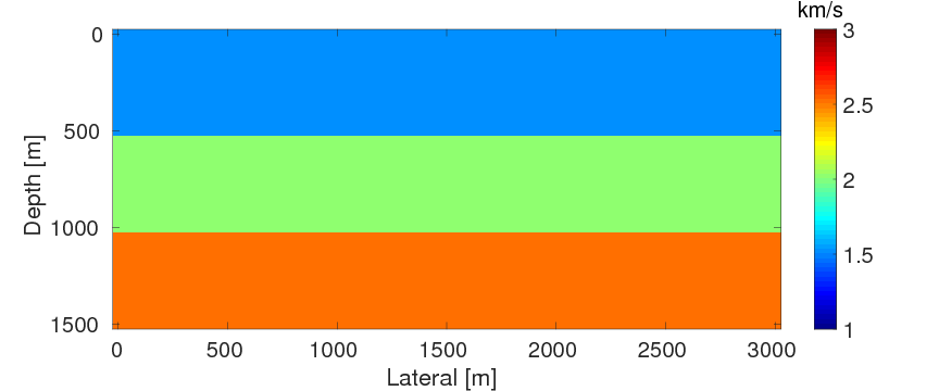
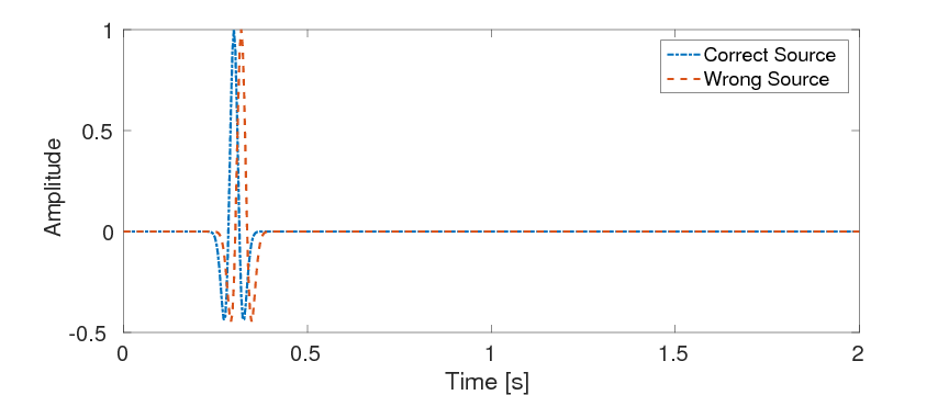
A well-known problem of the conventional adjoint-state method is that the resulting optimization problem may have local minima in common situations where the starting model for the velocity is not known accurately enough. As argued by van Leeuwen and Herrmann ({2013}), this sensitivity to the starting model is due to the fact that the adjoint-state method eliminates the wave-equation constraint by explicitly solving it, which results in an objective function that is highly nonlinear in the unknown medium parameters. To mitigate the problem of these local minima, van Leeuwen and Herrmann ({2013}) and van Leeuwen and Herrmann (2015) proposed a penalty formulation instead, where the wave-equation constraint is replaced by a weak constraint in the form of an \(\ell_2\)-norm penalty. This method is known as wavefield-reconstruction inversion (WRI) (van Leeuwen and Herrmann, {2013}, 2015). Compared to the adjoint-state method, WRI relaxes the wave-equation constraint by introducing the wavefields as auxiliary variables and adding a penalty term to the data misfit. This idea of extending the search space was also recently utilized by Huang et al. (2016), where an additional source term is introduced as the auxiliary variable. Both of these approaches are more or less equivalent and are successful in mitigating the effects of local minima, because the extended search space allows for fitting the observed data even in cases where the velocity model is incorrect. As a result, we can carry out the inversion with poorer initial models and start at higher frequencies (Peters et al., 2014). While these developments are encouraging, WRI does, as illustrated in Figure 1, require accurate information on the source functions. For instance, a small difference in the origin time of the source can lead to a significant deterioration of the inversion result (cf. Figure 1).
Recognizing this sensitivity to source functions, we propose a modified WRI framework with source estimation integrated, making the method applicable to field data. In this new formulation, we continue to solve an optimization problem but now one that has the source functions, medium parameters, and wavefields all as unknowns. For fixed medium parameters, we observe that the objective function of this optimization problem is quadratic with respect to both wavefields and source functions. As a result, if we collect the wavefield and source function for each source experiment into one single unknown vector variable, the optimization problem becomes an SNLLS problem with respect to the medium parameters and this new unknown variable. As before, we propose the variable projection method to solve the optimization problem by projecting out this new unknown variable during each iteration. After these least-squares problems, we compute single model updates either with the gradient descent or limited-memory Broyden–Fletcher–Goldfarb–Shanno (l-BFGS) method (Nocedal and Wright, 2006).
The outline of the paper is as follows. In the methodology section, we first start with a review of the source estimation technique for the conventional FWI using the variable projection method. Next, we introduce the standard WRI and propose our method for WRI source estimation. We conclude by presenting a computationally efficient implementation, which we evaluate on several synthetic examples to highlight the benefits of our approach.
Methodology
FWI with source estimation
During FWI, we solve the following least-squares problem for the discretized \(\ngrid\)-dimensional unknown medium parameters, squared slowness \(\mvec \in \RR^{\ngrid}\), which appear as coefficients in the acoustic time-harmonic wave-equation, i.e., \[ \begin{equation} \begin{split} \minimize_{\uvec,\,\mvec}\frac{1}{2}\sum_{i=1}^{\nsrc}\sum_{j=1}^{\nfreq}\|\P_{i}\uvec_{i,j}-{\d}_{i,j}\|^{2}_{2} \\ \hspace{8mm} \text{ subject to } \A_{j}(\mvec)\uvec_{i,j} = \qvec_{i,j}. \end{split} \label{FWI} \end{equation} \] Here, the \(i,j\)’s represent the source and frequency indices, and the vector \(\d \in \CC^{\nfreq \times \nsrc \times \nrcv}\) represents monochromatic Fourier transformed data collected at \(\nrcv\) receiver locations from \(\nsrc\) seismic sources and sampled at \(\nfreq\) frequencies. The matrix \(\A_{j}(\mvec) = \omega_{j}^{2}\text{diag}(\mvec) + \Delta\) is the discretized Helmholtz matrix at angular frequency \(\omega_{j}\). The symbol \(\Delta\) represents the discretized Laplacian operator and the matrix \(\P_{i}\) corresponds to a restriction operator for the receiver locations. Finally, the vectors \(\qvec_{i,j}\) and \(\uvec_{i,j}\) denote the unknown monochromatic source term at the \(i^{\text{th}}\) source location and \(j^{\text{th}}\) frequency and the corresponding wavefield, respectively. For simplicity, we omit the dependence of \(\A_j(\mvec)\) on the discretized squared slowness vector \(\mvec\) from now onwards.
Since the \(\A_j\)’s are square matrices, we can eliminate the variable \(\uvec\) by solving the discretized partial-differential equation (PDE) explicitly, leading to the so-called adjoint-state method, which has the following reduced form (Virieux and Operto, 2009): \[ \begin{equation} \minimize_{\mvec}\fred(\mvec)=\frac{1}{2}\sum_{i=1}^{\nsrc}\sum_{j=1}^{\nfreq}\|\P_{i}\A_{j}^{-1}\qvec_{i,j}-{\d}_{i,j}\|^{2}_{2}. \label{FWI2} \end{equation} \] In this form, the source function \(\qvec\) is assumed to be available. However, in practice, while spatial locations of the sources are often known quite accurately, the source function is generally unknown. If we ignore spatial directivity of the sources, we can handle this situation in the context of FWI by incorporating the source function through setting \(\qvec_{i,j} = \alpha_{i,j}\mathbf{e}_{i,j}\) in the frequency-domain, where \(\alpha_{i,j}\) is a complex number representing the frequency-dependent source weight for the \(i^{\text{th}}\) source experiment at the \(j^{\text{th}}\) frequency. In this expression, the symbol \(\mathbf{e}_{i,j}\) represents a unit vector that equals one at the source location and zero elsewhere. When we substitute \(\qvec_{i,j} = \alpha_{i,j}\mathbf{e}_{i,j}\) into the objective function in equation \(\ref{FWI2}\), we arrive at an optimization problem with two unknown variables, i.e., we have \[ \begin{equation} \minimize_{\mvec,\alpha}\fredover(\mvec,\,\alpha)=\frac{1}{2}\sum_{i=1}^{\nsrc}\sum_{j=1}^{\nfreq}\|\P_{i}\A_{j}^{-1}\alpha_{i,j}\mathbf{e}_{i,j}-{\d}_{i,j}\|^{2}_{2}, \label{FWI_Src} \end{equation} \] where the vector \(\alpha\, = \, \{\alpha_{i,j}\}_{1 \leq i \leq \nsrc, 1 \leq j \leq \nfreq}\) collects all the unknown source weights.
To solve the optimization problem in equation \(\ref{FWI_Src}\), one straightforward approach is to compute the gradient of the objective function \(\fredover\) with respect to \(\mvec\) and \(\alpha\), i.e., \[ \begin{equation} \begin{split} \overline{\gvec}_{\text{red}}(\mvec,\,\alpha) = \begin{bmatrix} \nabla_{\mvec} \overline{f}_{\text{red}}(\mvec,\alpha) \\ \nabla_{\alpha} \overline{f}_{\text{red}}(\mvec,\alpha) \end{bmatrix}, \end{split} \label{G_FWI_Src} \end{equation} \] and update \(\mvec\) and \(\alpha\) alternately (Zhou and Greenhalgh, 2003) or simultaneously (Liu et al., 2008). While relatively straightforward to compute, this formulation may result in converging to a local minimum, which requires a very good initial guess of \(\alpha\) to avoid. Moreover, while the gradients \(\nabla_{\mvec} \overline{f}_{\text{red}}(\mvec,\alpha)\) and \(\nabla_{\alpha} \overline{f}_{\text{red}}(\mvec,\alpha)\) seemingly provide all information that we would need to drive the inversion, their amplitudes may also differ significantly in scale. An undesired consequence of this mismatch between the two gradients is that the optimization may tend to primarily update the variable with the larger gradient contribution resulting in small updates for the other variable. This behavior may slow down the convergence, and the small updates may lead to errors that end up in the other variable resulting in a poor solution. Although we might mitigate this problem by manually scaling the two variables and the corresponding gradients to the approximately same levels, the crosstalk between \(\mvec\) and \(\alpha\) may lead to more local minima in the objective function, resulting in the requirement of a good initial guess of \(\alpha\) to ensure a successful inversion (M. Li et al., 2013).
Source estimation with the variable projection method
An alternative approach to solving the optimization problem in equation \(\ref{FWI_Src}\) is to use the so-called variable projection method (Golub and Pereyra, 2003) to project out the source weights \(\alpha\) during each iteration (Aravkin and van Leeuwen, 2012; M. Li et al., 2013). The variable projection method is designed to solve SNLLS problems, which permit the following standard expression: \[ \begin{equation} \minimize_{\theta,\, \xvec}f(\theta,\xvec)=\frac{1}{2}\| \Phi(\theta)\xvec -\yvec\|^2, \label{SNLLS} \end{equation} \] where the matrix \(\Phi(\theta)\) varies (nonlinearly) with respect to the variable vector \(\theta\). The vectors \(\xvec\) and \(\yvec\) represent a linear variable and the observations, respectively. More specifically, we can observe that the FWI problem with source estimation in equation \(\ref{FWI_Src}\) is a special case of SNLLS problems by setting \[ \begin{equation} \theta = \mvec, \quad \xvec_{i,j} = \alpha_{i,j}, \quad \yvec_{i,j} = {\d}_{i,j}, \quad \text{and} \quad \Phi_{i,j}(\theta) = \P_{i}\A_{j}^{-1}\evec_{i,j}, \label{FWIsrcVar1} \end{equation} \] for each pair of \((i,j)\). In this case, the vectors \(\xvec\) and \(\yvec\) are block vectors containing all \(\{\xvec_{i,j}\}_{1 \leq i \leq \nsrc, 1 \leq j \leq \nfreq}\) and \(\{\yvec_{i,j}\}_{1 \leq i \leq \nsrc, 1 \leq j \leq \nfreq}\). Likewise, \(\Phi(\theta)\) is a block-diagonal matrix.
When introducing the variable projection method, it is often useful to recognize that for fixed \(\theta\), the objective function \(f(\theta,\xvec)\) becomes quadratic with respect to \(\xvec\). As a consequence, the variable \(\xvec\) has a closed-form optimal least-squares solution \(\overline{\xvec}(\theta)\) that minimizes the objective \(f(\theta,\xvec)\): \[ \begin{equation} \overline{\xvec}(\theta) = \big (\Phi(\theta)^{\top}\Phi(\theta)\big )^{-1}\Phi(\theta)^{\top}\yvec, \label{VpSub} \end{equation} \] where the symbol \(^{\top}\) denotes the (complex-conjugate) transpose. For each pair of \((i,j)\), we now have \[ \begin{equation} \overline{\xvec}_{i,j}(\theta) = \big (\Phi_{i,j}(\theta)^{\top}\Phi_{i,j}(\theta)\big )^{-1}\Phi_{i,j}(\theta)^{\top}\yvec_{i,j}. \label{VpSub2} \end{equation} \] By substituting equation \(\ref{VpSub}\) into equation \(\ref{SNLLS}\), we project out the variable \(\xvec\) by the optimal solution \(\overline{\xvec}(\theta)\) and arrive at a reduced optimization problem over \(\theta\) alone, i.e., we have \[ \begin{equation} \minimize_{\theta}\overline{f}(\theta) = f\big (\theta,\overline{\xvec}(\theta)\big ) = \|\Big (\Imat - \Phi(\theta)\big (\Phi(\theta)^{\top}\Phi(\theta)\big )^{-1}\Phi(\theta)^{\top}\Big )\yvec\|^2. \label{Vpf2} \end{equation} \] The gradient of the reduced objective function \(\overline{f}(\theta)\) can be computed via the chain rule, yielding \[ \begin{equation} \overline{\gvec}(\theta) = \nabla_{\theta}\overline{f}(\theta) =\nabla_{\theta} {f}\big (\theta,\overline{\xvec}(\theta)\big )=\nabla_{\theta} f(\theta,\xvec)\rvert_{\xvec=\overline{\xvec}(\theta)} + \nabla_{\xvec}f(\theta,\xvec)\rvert_{\xvec=\overline{\xvec}(\theta)}\nabla_{\theta}\xvec. \label{VpfG} \end{equation} \] Note that from the definition of \(\overline{\xvec}(\theta)\), we have \[ \begin{equation} \nabla_{\xvec} f(\theta,\xvec)\rvert_{\xvec=\overline{\xvec}(\theta)} = 0. \label{ImpDf} \end{equation} \] With this equality, the gradient in equation \(\ref{VpfG}\) can be written as: \[ \begin{equation} \overline{\gvec}(\theta) = \nabla_{\theta} f(\theta,\xvec)\rvert_{\xvec=\overline{\xvec}(\theta)}. \label{VpfG2} \end{equation} \] Equation \(\ref{VpfG2}\) implies that although the optimal solution \(\overline{\xvec}(\theta)\) is a function of \(\theta\), the construction of the gradient \(\overline{\gvec}(\theta)\) does not need to include the cross-derivative term \(\nabla_{\xvec}f(\theta,\xvec)\rvert_{\xvec=\overline{\xvec}(\theta)}\nabla_{\theta}\xvec\) by the virtue of equation \(\ref{ImpDf}\).
As shown by Aravkin and van Leeuwen (2012) and van Leeuwen et al. (2014), we can through substituting equation \(\ref{FWIsrcVar1}\) into equations \(\ref{VpSub}\), \(\ref{Vpf2}\), and \(\ref{VpfG2}\) successfully project out the source weights by computing the optimal source weight \(\alpha_{i,j}(\mvec)\) for each source and frequency: \[ \begin{equation} \overline{\alpha}_{i,j}(\mvec) = \frac{\overline{\d}_{i,j}^{\top}\d_{i,j}}{\overline{\d}_{i,j}^{\top}\overline{\d}_{i,j}}, \quad \text{with} \quad \overline{\d}_{i,j} = \P_{i}\A_{j}^{-1}\evec_{i,j}, \label{FWIAlpha} \end{equation} \] and arrive at minimizing the following reduced objective: \[ \begin{equation} \minimize_{\mvec}\tilde{f}_{\text{red}}(\mvec) = \fredover\big (\mvec,\overline{\alpha}(\mvec)\big ), \label{FWIsrcVar} \end{equation} \] with a gradient given by \[ \begin{equation} \tilde{\gvec}_{\text{red}}(\mvec) = \nabla_{\mvec} \overline{f}_{\text{red}}(\mvec,\alpha)\rvert_{\alpha=\overline{\alpha}(\mvec)}. \label{FWIsrcVarG} \end{equation} \] Compared to the objective function \(\overline{f}_{\text{red}}(\mvec,\alpha)\) in equation \(\ref{FWI_Src}\), the objective function \(\tilde{f}_{\text{red}}(\mvec)\) only depends on \(\mvec\). As a consequence, we avoid having to optimize over two different variables that differ in scale. Moreover, because the objective \(\tilde{f}_{\text{red}}(\mvec)\) is source-independent, the optimization with it does not require any initial guesses of the source weights, while the optimization with the objective \(\overline{f}(\mvec,\alpha)\) does need a sufficiently accurate initial guess to ensure reaching the correct solution. Empirically, M. Li et al. (2013) showed the outperformances of minimizing \(\tilde{f}_{\text{red}}(\mvec)\) over minimizing \(\overline{f}(\mvec,\alpha)\), especially when the data contain noise.
WRI with source estimation
Introduction of WRI
In the conventional FWI or adjoint-state method in equation \(\ref{FWI2}\), the dependence of the objective function \(\fred(\mvec)\) on \(\mvec\) runs through the nonlinear operator \(\A_{j}^{-1}\qvec_{i,j}\), instead of via the original linear operator \(\A_{j}\uvec_{i,j}\) in equation \(\ref{FWI}\). As a result, the price we pay is that the objective function \(\fred(\mvec)\) becomes highly nonlinear in \(\mvec\). The gain, of course, is that we no longer have to optimize over the wavefields. However, this gain is perhaps a bit short-lived, because the reduced objective function \(\fred(\mvec)\) may contain local minima (Warner et al., 2013), which introduces more difficulties in the search for the best medium parameters using the local derivative information only.
To make FWI less susceptible to these parasitic minima, van Leeuwen and Herrmann ({2013}) and van Leeuwen and Herrmann (2015) proposed WRI—a penalty formulation of FWI that reads \[ \begin{equation} \minimize_{\mvec, \, \uvec} \fpen(\mvec,\uvec)=\frac{1}{2}\sum_{i=1}^{\nsrc}\sum_{j=1}^{\nfreq}\left(\|\P_{i}\uvec_{i,j}-{\d}_{i,j}\|^{2}_{2} + \lambda^{2}\|\A_{j}\uvec_{i,j}-\qvec_{i,j}\|^{2}_{2}\right). \label{WRI} \end{equation} \] In this optimization problem, we keep the wavefields \(\uvec\) as unknown variables instead of eliminating them as in FWI, i.e., we replace the PDE constraint by an \(\ell_2\)-norm penalty term. The scalar parameter \(\lambda\) controls the balance between the data and the PDE misfits. As \(\lambda\) increases, the wavefield is more tightly constrained by the wave-equation, and the objective function \(\fpen(\mvec,\uvec)\) in equation \(\ref{WRI}\) converges to the objective function of the reduced problem in equation \(\ref{FWI2}\) (van Leeuwen and Herrmann, 2015). Different from the nonlinear objective function of the reduced problem in equation \(\ref{FWI2}\), the WRI objective \(\fpen(\mvec,\uvec)\) is a bi-quadratic function with respect to \(\mvec\) and \(\uvec\), i.e., for fixed \(\mvec\), the objective \(\fpen(\mvec,\uvec)\) is quadratic with respect to \(\uvec\) and vice versa. In addition, van Leeuwen and Herrmann ({2013}) and van Leeuwen and Herrmann (2015) indicated that WRI explores a larger search space by not satisfying the PDE constraints exactly, which results in that WRI is less “nonlinear” and may contain less local minima compared to the conventional adjoint-state method.
In the optimization problem of equation \(\ref{WRI}\), both the wavefields \(\uvec\) and medium parameters \(\mvec\) are unknown. Searching for both \(\uvec\) and \(\mvec\) by methods like gradient-descent and l-BFGS method requires storing the two unknown variables. However, the memory cost of storing \(\uvec\) can be extremely large, because \(\uvec \in \CC^{\ngrid\times\nfreq\times\nsrc}\). To mitigate the storage cost, van Leeuwen and Herrmann ({2013}) and van Leeuwen and Herrmann (2015) noticed that the optimization problem in equation \(\ref{WRI}\) is also a special case of SNLLS problems and applied the variable projection method to solve it. Indeed, we have \[ \begin{equation} \begin{split} \theta = \mvec, \quad \xvec_{i,j} = \uvec_{i,j}, \quad \yvec_{i,j} = \begin{bmatrix} \lambda \qvec_{i,j} \\ {\d}_{i,j} \end{bmatrix}, \quad \text{and} \quad \Phi_{i,j}(\theta) = \begin{bmatrix} \lambda \A_{j} \\ \P_{i} \end{bmatrix}. \end{split} \label{WRIavr1} \end{equation} \] Therefore, after substituting equation \(\ref{WRIavr1}\) into equations \(\ref{VpSub}\), \(\ref{Vpf2}\), and \(\ref{VpfG2}\), we can successfully project out the wavefields \(\uvec\) by computing the optimal wavefield \(\overline{\uvec}_{i,j}(\mvec)\) for each source and frequency: \[ \begin{equation} \overline{\uvec}_{i,j}(\mvec) = \left( \lambda^2\A_{j}^{\top}\A_{j} + \P_{i}^{\top}\P_{i} \right)^{-1}\left(\lambda^2\A_{j}^{\top}\qvec_{i,j} +\P_{i}^{\top}\d_{i,j} \right), \label{WRIU} \end{equation} \] and arrive at minimizing the following reduced objective: \[ \begin{equation} \begin{aligned} \minimize_{\mvec}\overline{f}_{\text{pen}}(\mvec) &= \fpen\big (\mvec,\overline{\uvec}(\mvec)\big )\\ &=\frac{1}{2}\sum_{i=1}^{\nsrc}\sum_{j=1}^{\nfreq}\left(\|\P_{i}\overline{\uvec}_{i,j}(\mvec)-{\d}_{i,j}\|^{2}_{2} + \lambda^{2}\|\A_{j}\overline{\uvec}_{i,j}(\mvec)-\qvec_{i,j}\|^{2}_{2}\right), \end{aligned} \label{WRIred} \end{equation} \] with a gradient given by \[ \begin{equation} \overline{\gvec}_{\text{pen}}(\mvec) =\sum_{i=1}^{\nsrc}\sum_{j=1}^{\nfreq}\lambda^2\omega_{i}^{2}\text{diag}\Big (\text{conj}\big (\overline{\uvec}_{i,j}(\mvec)\big )\Big )\big(\A_{j}\overline{\uvec}_{i,j}(\mvec)-{\qvec}_{i,j}\big). \label{WRIG} \end{equation} \] Here the term \(\text{diag} \Big (\text{conj}\big (\overline{\uvec}_{i,j}(\mvec)\big ) \Big)\) represents a diagonal matrix with the elements of the complex conjugate of the vector \({\overline{\uvec}}_{i,j}(\mvec)\) on the diagonal. With the projection of the wavefields \(\uvec\) in equation \(\ref{WRIU}\), the new reduced objective \(\overline{f}_{\text{pen}}(\mvec)\) varies only with respect to the variable \(\mvec\). As a result, we do not need to store the \(\uvec\)’s reducing the storage costs from \(\mathcal{O}(\ngrid \times (\nfreq \times \nsrc + 1))\) to \(\mathcal{O}(\ngrid)\).
Source estimation for WRI
The standard formulation of WRI in equation \(\ref{WRI}\) does not take situations with unknown source functions into account. When the source functions are unknown, we face to solve an optimization problem with three unknown variables, i.e., we have \[ \begin{equation} \minimize_{\mvec,\, \uvec,\, \alpha} \fpen(\mvec,\,\uvec,\,\alpha)=\frac{1}{2}\sum_{i=1}^{\nsrc}\sum_{j=1}^{\nfreq}\left(\|\P_{i}\uvec_{i,j}-{\d}_{i,j}\|^{2}_{2} + \lambda^{2}\|\A_{j}\uvec_{i,j}-\alpha_{i,j}\mathbf{e}_{i,j}\|^{2}_{2}\right), \label{ObjPen} \end{equation} \] where the vector \(\alpha = \{\alpha_{i,j}\}_{1 \leq i \leq \nsrc, 1 \leq j \leq \nfreq}\) contains all the source weights.
Because this new objective \(\fpen(\mvec,\,\uvec,\,\alpha)\) contains more than two unknowns, it no longer corresponds to a standard SNLLS problem, so we cannot directly apply the variable projection method to solve it. One simple approach that comes to mind to convert the problem in equation \(\ref{ObjPen}\) to a standard SNLLS problem would be to reduce the number of unknown variables by collecting two of the three variables into a new variable. Since for fixed \(\mvec\) and \(\alpha\), \(\fpen(\mvec,\,\uvec,\,\alpha)\) is still quadratic with respect to \(\uvec\), the most straightforward approach would be to lump the medium parameters \(\mvec\) and the source weights \(\alpha\) together. During each iteration, we can apply the variable projection method to project out \(\uvec\), yielding an objective function \(\tilde{f}(\mvec,\,\alpha)\) with respect to both \(\mvec\) and \(\alpha\). However, as discussed in the context of FWI with source estimation, minimizing \(\tilde{f}(\mvec,\,\alpha)\) by either simultaneously or alternately updating \(\mvec\) and \(\alpha\) would face the convergence-related problems caused by the crosstalk between the two unknowns and the mismatch of their amplitudes. Additionally, a straightforward application of the variable projection method to project out \(\alpha\) from \(\tilde{f}(\mvec,\,\alpha)\) is not viable, because it destroys the underlying assumption of the projection of \(\uvec\), i.e., \(\nabla_{\uvec} \fpen(\mvec,\uvec,\alpha)\rvert_{\uvec=\overline{\uvec}(\mvec,\alpha)} \neq 0\) with the projected \(\alpha\).
To address the challenge arising from the different amplitude scales of \(\mvec\) and \(\alpha\) and their gradients, we propose another strategy to reduce the original problem in equation \(\ref{ObjPen}\). Instead of collecting \(\mvec\) and \(\alpha\) together, we lump \(\uvec\) and \(\alpha\) into a single vector \(\xvec\). To understand the potential advantage of this alternative strategy, let us rewrite the optimization problem in equation \(\ref{ObjPen}\) as \[ \begin{equation} \begin{aligned} \minimize_{\mvec,\,\uvec,\, \alpha}\fpen(\mvec,\uvec,\alpha)&=\frac{1}{2}\sum_{i=1}^{\nsrc}\sum_{j=1}^{\nfreq}\|\begin{bmatrix} \lambda{\A_{j}} & -\lambda{\mathbf{e}_{i,j}} \\ \P_{i} & 0 \end{bmatrix} \begin{bmatrix} {\uvec}_{i,j} \\ {\alpha}_{i,j} \end{bmatrix} - \begin{bmatrix} 0 \\ {\d}_{i,j} \end{bmatrix}\|^2 \\ &=\frac{1}{2}\sum_{i=1}^{\nsrc}\sum_{j=1}^{\nfreq}\|\begin{bmatrix} \lambda{\A_{j}} & -\lambda{\mathbf{e}_{i,j}} \\ \P_{i} & 0 \end{bmatrix} \xvec_{i,j} - \begin{bmatrix} 0 \\ {\d}_{i,j} \end{bmatrix}\|^2 \\ :&=\fpent(\mvec,\xvec). \end{aligned} \label{SimpObj} \end{equation} \] For fixed \(\mvec\), the objective function \(\fpent(\mvec,\xvec)\) continues to be quadratic in the new variable \(\xvec\), where \(\uvec\) and \(\alpha\) are grouped together. As a result, we can rewrite the optimization problem in equation \(\ref{SimpObj}\) into the standard SNLLS form (see equation \(\ref{SNLLS}\)) when we use the following notations: \[ \begin{equation} \begin{aligned} \theta = \mvec , \quad \xvec_{i,j} = \begin{bmatrix} \uvec_{i,j} \\ \alpha_{i,j} \end{bmatrix}, \quad \yvec_{i,j} = \begin{bmatrix} \mathbf{0} \\ {\d}_{i,j} \end{bmatrix}, \quad \text{and} \quad \Phi_{i,j}(\theta) = \begin{bmatrix} \lambda \A_{j} & -\lambda\evec_{i,j} \\ \P_{i} & \mathbf{0} \end{bmatrix}. \end{aligned} \label{WRISrcGroup2} \end{equation} \] Now by substituting the notations in equation \(\ref{WRISrcGroup2}\) into equation \(\ref{VpSub2}\), we can apply the variable projection method again to project out \(\xvec\) from the objective function \(\fpent(\mvec,\xvec)\) for fixed \(\mvec\) by computing the optimal solution \[ \begin{equation} \begin{aligned} \overline{\xvec}_{i,j}(\mvec) = \begin{bmatrix} \overline{\uvec}_{i,j}(\mvec) \\ \overline{\alpha}_{i,j}(\mvec) \end{bmatrix} = \begin{bmatrix} \lambda^{2}{\A_{j}^{\top}\A_{j}}+\P_{i}^{\top}\P_{i} & -\lambda^{2}\A^{\top}_{j}{\mathbf{e}_{i,j}} \\ -\lambda^{2}\mathbf{e}_{i,j}^{\top}\A_{j} & \lambda^{2}\mathbf{e}_{i,j}^{\top}\mathbf{e}_{i,j} \end{bmatrix}^{-1} \begin{bmatrix} \P_{i}\d_{i,j} \\ \mathbf{0}\end{bmatrix}. \end{aligned} \label{OptUandalpha2} \end{equation} \] The linear system in equation \(\ref{OptUandalpha2}\) is solvable if and only if the rank of the matrix \(\Phi_{i,j}(\theta)\) in equation \(\ref{WRISrcGroup2}\) is \(\ngrid + 1\), which requires \[ \begin{equation} \P_{i}\A_{j}^{-1}\evec_{i,j} \neq 0. \label{solvability} \end{equation} \] In fact, this means that the wavefields corresponding to a point source do not vanish at all the receiver locations simultaneously, which holds in almost all seismic situations. Indeed, even in the extremely rare situation where a source is made nearly “silent” or non-radiating due to its surrounding geological structures, we can simply discard this source in the inversion to avoid inverting a rank deficient matrix. After the projection in equation \(\ref{OptUandalpha2}\), we obtain an objective function that only depends on \(\mvec\): \[ \begin{equation} \hat{f}(\mvec) = \fpen\big (\mvec,\overline{\uvec}(\mvec),\overline{\alpha}(\mvec)\big ), \label{VarObj2} \end{equation} \] whose gradient \(\hat{\gvec}(\mvec)\) can be derived as \[ \begin{equation} \begin{aligned} \hat{\gvec}(\mvec) &= \nabla_{\mvec}\hat{f}(\mvec) = \nabla_{\mvec}\fpen(\mvec,\uvec,\alpha)\rvert_{\uvec=\overline{\uvec}(\mvec),{\alpha}=\overline{\alpha}(\mvec)} \\ &=\sum_{i=1}^{\nsrc}\sum_{j=1}^{\nfreq}\lambda^2\omega_{i}^{2}\text{diag}\Big (\text{conj}\big (\overline{\uvec}_{i,j}(\mvec)\big )\Big )\big (\A_{j}\overline{\uvec}_{i,j}(\mvec)-\overline{\alpha}_{i,j}(\mvec){\evec}_{i,j}\big ). \end{aligned} \label{VarG2} \end{equation} \] As a result, we avoid optimizing over two different variables that differ in scale. Moreover, the optimization with \(\hat{f}(\mvec)\) does not require any initial guesses of the source weights.
Optimization scheme
With the gradient \(\hat{\gvec}(\mvec)\) we derived in the previous section we can compute updates for the medium parameters via the steepest-descent method (Nocedal and Wright, 2006): \[ \begin{equation} \mvec_{k+1} = \mvec_{k} - \beta_{k}\hat{\gvec}(\mvec_{k}). \label{gradient-descent} \end{equation} \] Here, the value \(\beta_{k}\) is an appropriately chosen step length at the \(k^{\text{th}}\) iteration, which requires a line search to determine. Even with an optimized step length, as a first-order method, the steepest-descent method can be slow. To speed up the convergence, second-order methods including Newton method, Gauss-Newton method, and quasi-Newton method may be more desirable (Pratt, 1999; Akcelik, 2002; Askan et al., 2007). During each iteration, Newton method and Gauss-Newton method use the full or Gauss-Newton Hessian to compute the update direction. However, the construction and inversion of the full or Gauss-Newton Hessian for both FWI (Pratt, 1999) and WRI (van Leeuwen and Herrmann, 2015) involve a large amount of additional PDE solves, which makes these two methods less attractive in this context. On the other hand, the quasi-Newton method, especially the l-BFGS method (Nocedal and Wright, 2006; Brossier et al., 2009; van Leeuwen and Herrmann, 2013), utilizes the gradient at the current iteration \(k\) and a few previous gradients (typically, 3-20 iterations) to construct an approximation of the inverse of the Hessian. Hence, except for the increased memory, the l-BFGS method constructs the approximation of the inverse of the Hessian for free. For this reason, we use the l-BFGS method as our optimization scheme and denote the l-BFGS update as \[ \begin{equation} \mvec_{k+1} = \mvec_{k} -\beta_{k}\Hmat(\mvec_{k})^{-1}\hat{\gvec}(\mvec_{k}), \label{Modelupdate} \end{equation} \] where the matrix \(\Hmat(\mvec_{k})\) is the l-BFGS Hessian and the step length \(\beta_{k}\) is determined by a weak Wolfe line search. We give a detailed description of the l-BFGS method for the proposed WRI framework with source estimation in Algorithm 1.
1. Initialization with an initial model \(\mvec_{0}\)
2. for \(k = 1 \rightarrow \niter\)
3. for \(j = 1 \rightarrow \nfreq\)
4. for \(i = 1 \rightarrow \nsrc\)
5. Compute \(\overline{\uvec}_{i,j}(\mvec_{k})\) and \(\overline{\alpha}_{i,j}(\mvec_{k})\) by equation \(\ref{OptUandalpha2}\)
6. end
7. end
8. Compute \(\hat{f}_{k}\) and \({\hat{\gvec}}_{k}\) by equations \(\ref{VarObj2}\) and \(\ref{VarG2}\)
9. Apply l-BFGS Hessian with history size \(n_{\text{his}}\)
10. \(\pvec_{k} = \text{lbfgs}(-{\hat{\gvec}}_{k}, \{\tvec_{l}\}^{k}_{l=k-n_{\text{his}}}, \{\svec_{l}\}^{k}_{l=k-n_{\text{his}}})\)
11. \(\{\mvec_{k+1}, {\hat{f}}_{k+1}, {\hat{\gvec}}_{k+1}\} = \text{line search}({\hat{f}}_{k}, {\hat{\gvec}}_{k}, \pvec_{k})\)
12. \(\tvec_{k+1} = \mvec_{k+1}-\mvec_{k}\)
13. \(\svec_{k+1} = {\hat{\gvec}}_{k+1}-{\hat{\gvec}}_{k}\)
14. end
Fast solver for WRI with source estimation
Most of the computational burden for the objective function and its gradient in equations \(\ref{VarObj2}\) and \(\ref{VarG2}\) lies within inverting the matrix \[ \begin{equation} \begin{aligned} \Cmat_{i,j}(\mvec) = \Phi_{i,j}(\mvec)^{\top}\Phi_{i,j}(\mvec) = \begin{bmatrix} \lambda^{2}{\A_{j}^{\top}\A_{j}}+\P_{i}^{\top}\P_{i} & -\lambda^{2}\A^{\top}_{j}{\mathbf{e}_{i,j}} \\ -\lambda^{2}\mathbf{e}_{i,j}^{\top}\A_{j} & \lambda^{2}\mathbf{e}_{i,j}^{\top}\mathbf{e}_{i,j} \end{bmatrix}. \end{aligned} \label{Cmat} \end{equation} \] For 2D problems, we can invert the matrix \(\Cmat_{i,j}(\mvec)\) by direct solvers such as the Cholesky method, while for 3D problems, we may need an iterative solver equipped with a proper preconditioner. In either case, following computational challenges arise from the fact that the matrix \(\Cmat_{i,j}(\mvec)\) differs from source to source and frequency to frequency. First, to apply the Cholesky method, we need to calculate the Cholesky factorization for each \(i\) and \(j\), i.e., for each source and frequency. As a result, the computational cost arrives at \(\mathcal{O}\big(\nsrc \times \nfreq \times (\ngrid^{3} + \ngrid^{2})\big )\), which prohibits the application to problems with a large number of sources. Second, for iterative solvers, because the matrix \(\Cmat_{i,j}(\mvec)\) varies with respect to \(i\) and \(j\), the corresponding preconditioner may as well as depend on \(i\) and \(j\). Therefore, we may have to design \(\nsrc \times \nfreq\) different preconditioners, which can be computationally difficult and intractable. Moreover, the additional terms \(-\lambda^{2}\A^{\top}_{j}{\mathbf{e}_{i,j}}\), \(-\lambda^{2}\mathbf{e}_{i,j}^{\top}\A_{j}\), and \(\lambda^{2}\mathbf{e}_{i,j}^{\top}\mathbf{e}_{i,j}\) may lead to the condition number of the matrix \(\Cmat_{i,j}\) worse than that of the matrix \(\lambda^{2}{\A_{j}^{\top}\A_{j}}+\P_{i}^{\top}\P_{i}\). As a result, without a good preconditioner, the projection procedure in the framework of WRI with source estimation may be much slower than that without source estimation.
To lighten the computational cost of inverting the matrix \(\Cmat_{i,j}(\mvec)\), we describe a new inversion scheme to implement the algorithm when the projection operator \(\P\) remains the same for all sources. This situation is common in ocean bottom node acquisition and the land acquisition where all sources “see” the same receivers. When we replace \(\P_i\) by a single \(\P\) in equation \(\ref{Cmat}\), the matrix \(\Cmat_{i,j}(\mvec)\) can be simplified as \[ \begin{equation} \begin{aligned} \Cmat_{i,j}(\mvec) = \begin{bmatrix} \lambda^{2}{\A_{j}^{\top}\A_{j}}+\P^{\top}\P & -\lambda^{2}\A^{\top}_{j}{\mathbf{e}_{i,j}} \\ -\lambda^{2}\mathbf{e}_{i,j}^{\top}\A_{j} & \lambda^{2}\mathbf{e}_{i,j}^{\top}\mathbf{e}_{i,j} \end{bmatrix}. \end{aligned} \label{Cmat2} \end{equation} \] Unfortunately, this matrix \(\Cmat_{i,j}(\mvec)\) still depends on the source and frequency indices, and a straightforward inversion still faces the aforementioned computational challenges. However, this form, equation \(\ref{Cmat2}\), allows us to use an alternative block matrix formula to invert \(\Cmat_{i,j}(\mvec)\). To arrive at this result, let us first write \(\Cmat_{i,j}(\mvec)\) in a simpler form \[ \begin{equation} \begin{aligned} \Cmat_{i,j}(\mvec) = \begin{bmatrix} \Mmat_1 & \Mmat_2 \\ \Mmat_3 & \Mmat_4 \end{bmatrix}, \end{aligned} \label{Cmat3} \end{equation} \] where the matrix \(\Mmat_1 = \lambda^{2}{\A_{j}^{\top}\A_{j}}+\P^{\top}\P\), the vector \(\Mmat_2 = \Mmat_{3}^{\top} = -\lambda^{2}\A^{\top}_{j}{\mathbf{e}_{i,j}}\), and the scalar \(\Mmat_4 = \lambda^{2}\mathbf{e}_{i,j}^{\top}\mathbf{e}_{i,j}\). Now if we apply the block matrix inversion formula (Bernstein, 2005) to compute \(\Cmat^{-1}_{i,j}(\mvec)\), we arrive at the following closed form analytical expression \[ \begin{equation} \begin{aligned} \Cmat^{-1}_{i,j}(\mvec) = \begin{bmatrix} (\Imat + \Mmat_{1}^{-1}\Mmat_{2}(\Mmat_{4}-\Mmat_{3}\Mmat_{1}^{-1}\Mmat_{2})^{-1}\Mmat_{3})\Mmat_{1}^{-1} & -\Mmat_{1}^{-1}\Mmat_{2}(\Mmat_{4}-\Mmat_{3}\Mmat_{1}^{-1}\Mmat_{2})^{-1} \\ -(\Mmat_{4}-\Mmat_{3}\Mmat_{1}^{-1}\Mmat_{2})^{-1}\Mmat_{3}\Mmat_{1}^{-1} & (\Mmat_{4}-\Mmat_{3}\Mmat_{1}^{-1}\Mmat_{2})^{-1} \end{bmatrix}. \end{aligned} \label{Cmat4} \end{equation} \] While complicated the right-hand side of this equation only involves the inversion of the source-independent matrix \(\Mmat_{1}\), all other terms are all scalar inversions that can be evaluated at negligible costs. Substituting equation \(\ref{Cmat4}\) into equation \(\ref{OptUandalpha2}\), we obtain an analytical solution for the optimal variable \[ \begin{equation} \begin{aligned} \overline{\xvec}_{i,j}(\mvec) &= \Cmat^{-1}_{i,j}(\mvec)\begin{bmatrix} \P^{\top}{\d}_{i,j} \\ 0 \end{bmatrix} \\ &= \begin{bmatrix} (\Imat + \Mmat_{1}^{-1}\Mmat_{2}(\Mmat_{4}-\Mmat_{3}\Mmat_{1}^{-1}\Mmat_{2})^{-1}\Mmat_{3})\Mmat_{1}^{-1}\P^{\top}{\d}_{i,j} \\ -(\Mmat_{4}-\Mmat_{3}\Mmat_{1}^{-1}\Mmat_{2})^{-1}\Mmat_{3}\Mmat_{1}^{-1}\P^{\top}{\d}_{i,j} \end{bmatrix}. \end{aligned} \label{AnlyOptX} \end{equation} \] In equation \(\ref{AnlyOptX}\), we have to invert two terms, i.e., \(\Mmat_{1}\) and \(\Mmat_{4}-\Mmat_{3}\Mmat_{1}^{-1}\Mmat_{2}\). Because \(\Mmat_{4}\) is a scalar, the term \((\Mmat_{4}-\Mmat_{3}\Mmat_{1}^{-1}\Mmat_{2})^{-1}\) is a scalar inversion, whose computational cost is negligible. Therefore, to construct \(\overline{\xvec}_{i,j}(\mvec)\), we only need to compute the following two vectors: \[ \begin{equation} \begin{aligned} \wvec_{1} &= \Mmat_{1}^{-1}\Mmat_{2} \\ &= -\lambda^{2}(\lambda^{2}{\A_{j}^{\top}\A_{j}}+\P^{\top}\P)^{-1}\A^{\top}_{j}{\mathbf{e}_{i,j}}, \end{aligned} \label{w1} \end{equation} \] and \[ \begin{equation} \begin{aligned} \wvec_{2} &= \Mmat_{1}^{-1}\P^{\top}{\d}_{i,j} \\ &= (\lambda^{2}{\A_{j}^{\top}\A_{j}}+\P^{\top}\P)^{-1}\P^{\top}{\d}_{i,j}. \end{aligned} \label{w2} \end{equation} \] From these two expressions, we can observe that the computation of the vectors \(\wvec_{1}\) and \(\wvec_{2}\) for each source is independent from that of other sources, therefore, we can sequentially compute them from source to source, yielding a negligible requirement of storing only 2 additional wavefields during the inversion. For each frequency, because the matrix \(\Mmat_{1}\) is source-independent, we only need one Cholesky factorization, whose computational cost is \(\mathcal{O}(\ngrid^{3})\). With the pre-computed Cholesky factors, for each source, solving \(\wvec_{1}\) and \(\wvec_{2}\) by equations \(\ref{w1}\) and \(\ref{w2}\) requires inverting the matrix \(\Mmat_{1}\) twice with a computational cost of \(\mathcal{O}(\ngrid^{2})\). Consequently, we reduce the total cost from \(\mathcal{O}\big (\nsrc \times \nfreq \times (\ngrid^{3} + \ngrid^{2})\big )\) to \(\mathcal{O}\big (\nfreq \times (\ngrid^{3} + 2 \times \nsrc \times \ngrid^{2})\big )\). As a reference, the computational complexity of WRI without source estimation is of a close order \(\mathcal{O}\big (\nfreq \times (\ngrid^{3} + \nsrc \times \ngrid^{2})\big )\) (van Leeuwen and Herrmann, 2015). A comparison of the computational complexity of WRI with and without source estimation using the Cholesky method is shown in Table 1. In this table, we refer to the scheme that directly inverts the matrix \(\Cmat_{i,j}(\mvec)\) as the old form, and refer to the proposed scheme in equation \(\ref{AnlyOptX}\) as the new form. Compared to the old form, instead of requiring \(\nsrc\) Cholesky factorizations, the proposed new form only requires \(1\) Cholesky factorization for each frequency, which significantly reduces the computational cost. Furthermore, besides reducing the cost for direct solvers, the proposed inversion scheme can also benefit iterative solvers. For each frequency, since all sources only need to invert the same matrix \(\Mmat_{1}\), the proposed new form avoids inverting the potentially ill-conditioned matrix \(\Cmat_{i,j}\) directly and only requires one preconditioner instead of \(\nsrc\), which significantly simplifies the projection procedure. In the following section of numerical experiments, we will only show the computational gain for direct solvers.
| nr. of Cholesky factorization | nr. of invertion with Cholesky factors | |
|---|---|---|
| w/o source estimation | 1 per frequency | 2 per source per frequency |
| w/ source estimation – old form | \(\nsrc\) per frequency | 2 per source per frequency |
| w/ source estimation – new form | 1 per frequency | 4 per source per frequency |
Numerical Examples
BG model with frequency-domain data
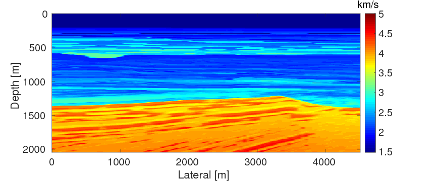
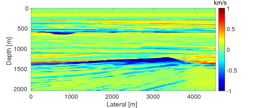
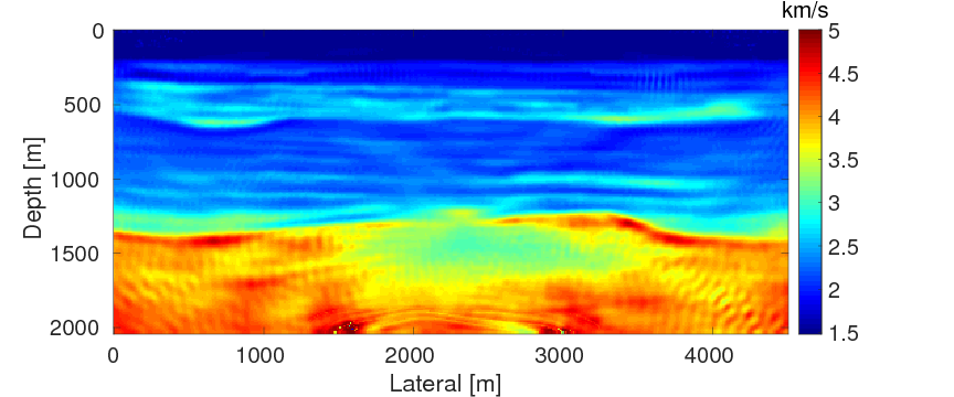
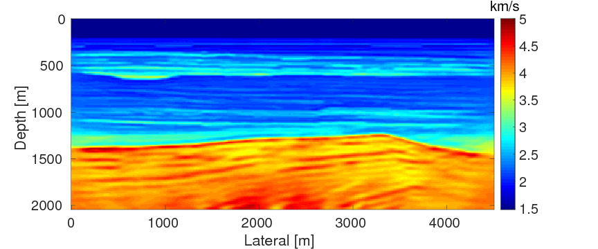
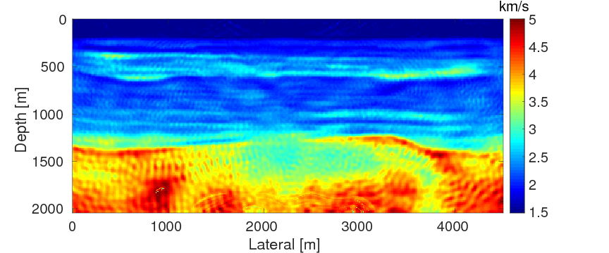
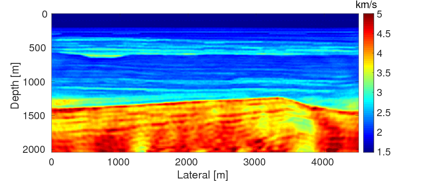
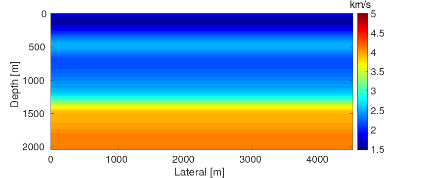
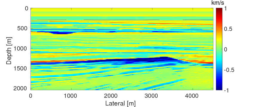
To compare the performance of the two source estimation methods for WRI described in the previous section, we conduct numerical experiments on a part of the BG compass model \(\mvec_{\text{t}}\) shown in Figure 2a, which is a geologically realistic model created by BG Group and has been widely used to evaluate performances of different FWI methods (X. Li et al., 2012; van Leeuwen and Herrmann, 2013). We will refer to the method that combines \(\mvec\) and \(\alpha\) as WRI-SE-MS and the one that combines \(\uvec\) and \(\alpha\) as WRI-SE-WS. For our discretization, we use an optimal 9-point finite-difference frequency-domain forward modeling code (Chen et al., 2013). Sources and receivers are positioned at the depth of \(z \, = \, 20 \, \mathrm{m}\) with a source distance of \(50 \, \mathrm{m}\) and a receiver distance of \(10 \, \mathrm{m}\), resulting a maximum offset of \(4.5\, \mathrm{km}\). Data is generated with a source function given by a Ricker wavelet centered at \(20 \, \mathrm{Hz}\) with a time shift of \(0.5 \, \mathrm{s}\). We do not model the free-surface, so the data contain no free-surface related multiples. As is commonly practiced (see e.g. Pratt (1999)), we perform frequency continuation using frequency bands ranging from \(\{2,\,2.5,\,3,\,3.5,\,4,\,4.5\} \, \mathrm{Hz}\) to \(\{27,\,27.5,\,28,\,28.5,\,29,\,29.5\} \, \mathrm{Hz}\) with an overlap of one frequency between every two consecutive bands. During the inversion, the result of the current frequency band serves as a warm starter for the inversion of the next frequency band. During each iteration, we also apply a point-wise bound constraint (Peters and Herrmann, 2016) to the update to ensure that each gridpoint of the model update remains within a geologically reasonable interval. In this experiment, because the lowest and highest velocities of the true model are \(1480 \, \mathrm{m/s}\) and \(4500 \, \mathrm{m/s}\), we set the interval of the bound constraint to be \([1300, \, 5000] \, \mathrm{m/s}\). The initial model \(\mvec_{0}\) (Figure 2b) is generated by smoothing the original model, followed by an average along the horizontal direction. The difference between the initial and true models is shown in Figure 2c. We use this initial model and apply the source estimation method proposed by Pratt (1999) to obtain an initial guess of the source weights for WRI-SE-MS. Because this guess minimizes the difference between the observed and predicted data with the initial model, it can be considered as the best choice, when there is no more additional information. For WRI-SE-WS, as described in the previous sections, it does not need an initial guess of the source weights. To control the computational load, we fix the maximum number of l-BFGS iterations to be 20 for each frequency band. We select the penalty parameter \(\lambda = 1e4\) according to the selection criteria in van Leeuwen and Herrmann (2015) that optimizes the performance of WRI.

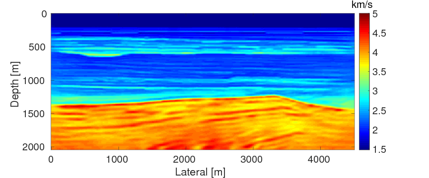
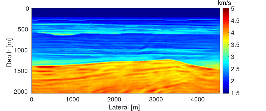
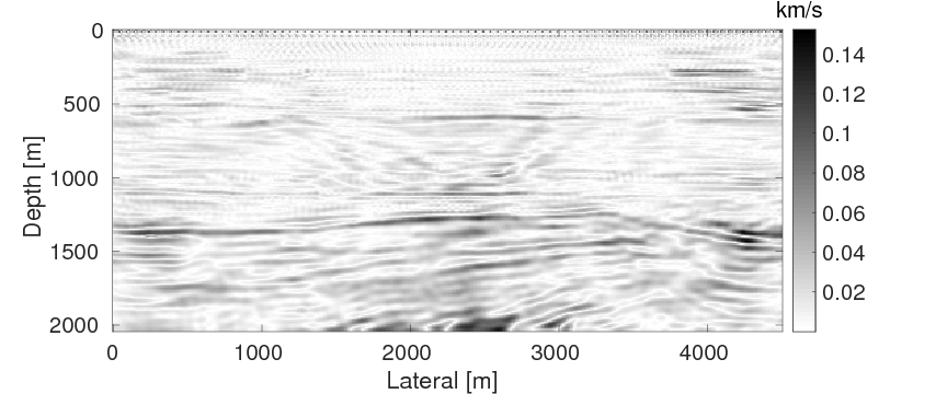
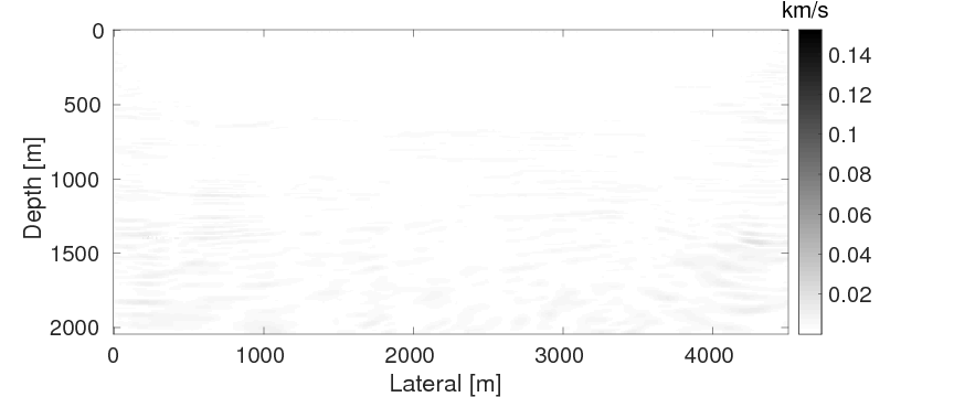
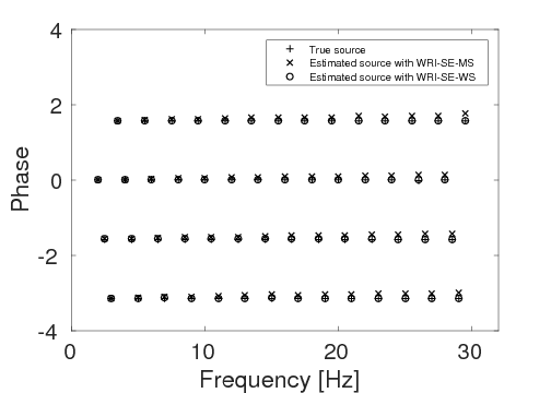
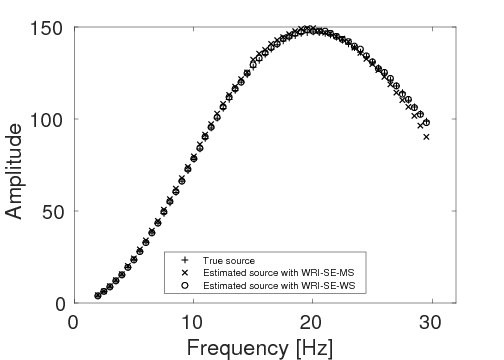
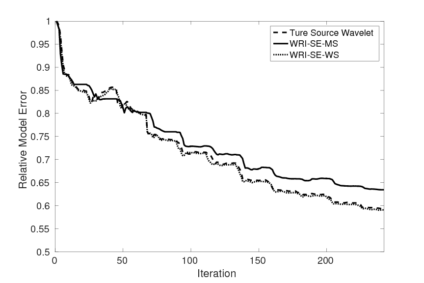
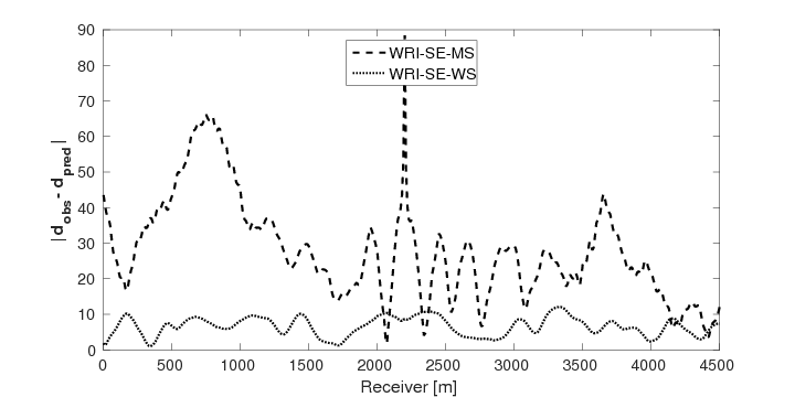
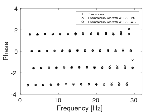
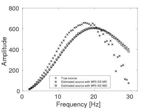
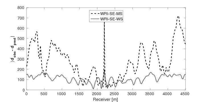
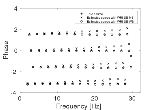
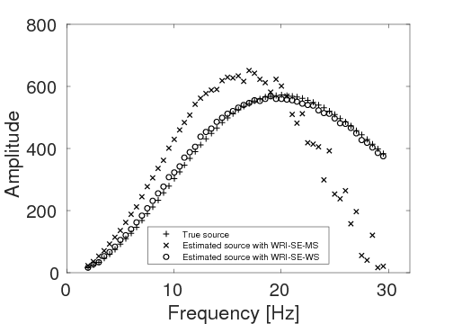
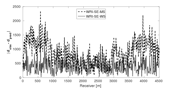
As a benchmark, we depict the inversion result obtained with the true source weights in Figure 3a. Figures 3b and 3c show the inversion results obtained by WRI-SE-MS and WRI-SE-WS, respectively. Figure 3d shows the difference between the results in Figures 3a and 3b, and Figure 3e displays the difference between the results in Figures 3a and 3c. We observe that while both the results obtained by WRI-SE-MS and WRI-SE-WS are close to the result obtained with the true source weights, the difference shown in Figure 3d is almost 10 times larger than that shown in Figure 3e. In addition, we compare the true source weights and the estimated source weights obtained with WRI-SE-MS and WRI-SE-WS in Figures 4a (phase) and 4b (amplitude). From these two figures, we observe that both methods can provide reasonable estimates of the source weights while the estimates with WRI-SE-WS contain smaller errors. These errors found in the source weights may result in the large model differences shown in Figure 3d. In Figure 5, we display the relative model errors \(\frac{\|\mvec_{\text{t}}-\mvec\|}{\|\mvec_{\text{t}}-\mvec_{0}\|}\) versus the number of iterations during the three inversions. The dashed, solid, and dotted curves correspond to inversions with the true source weights and those estimates using WRI-SE-MS and WRI-SE-WS. The relative model errors of WRI-SE-WS are almost the same as those using the true source weights, while the errors of WRI-SE-MS are clearly larger than the other ones. Figure 6 depicts a comparison of the data residuals corresponding to the inversion results of WRI-SE-MS and WRI-SE-WS. Clearly, the data residual of WRI-SE-WS is much smaller than that of WRI-SE-MS. In Table 2, we quantitatively compare the inversion results obtained by WRI-SE-MS and WRI-SE-WS in terms of the final model errors, source errors, and data residuals, which also illustrates the outperformances of WRI-SE-WS over WRI-SE-MS. These observations imply that compared to iteratively updating \(\alpha\), projecting out \(\alpha\) and \(\uvec\) together during each iteration can provide more accurate estimates of source weights, which further benefits the inversions of medium parameters.

| WRI-SE-MS | WRI-SE-WS | |
|---|---|---|
| \(\|\mvec_{\text{t}}-\mvec_{\text{f}}\|_{2}\) | 48 | 45 |
| \(\|\alpha_{\text{t}}-\alpha_{\text{f}}\|_{2}\) | \(9.3e2\) | \(8e1\) |
| \(\|\d_{\text{obs}} - \d_{\text{pred}}\|_{2}\) | \(6.6e3\) | \(1.5e3\) |
To evaluate the computational performance of the fast inversion scheme of WRI-SE-WS, we compare the time spent in evaluating one objective for three cases, namely (i) WRI without source estimation; (ii) WRI-SE-WS with the old form, equation \(\ref{OptUandalpha2}\); and (iii) WRI-SE-WS with the new form, equation \(\ref{AnlyOptX}\). The computational time for each of the three cases is \(94 \, \mathrm{s}\), \(2962 \, \mathrm{s}\), and \(190 \, \mathrm{s}\), respectively. As expected, case (iii) spends twice the amount of time as case (i), because of the additional PDE solves for each frequency and each source. As only one Cholesky factorization is required for case (iii), the computational time is only \(1/15\) of that for case (ii). This result illustrates that the proposed approach can estimate source weights in the context of WRI with a small computational overhead.
BG model with time-domain data
To test the robustness of the two source estimation techniques in less ideal situations, we perform the inversion tests on non-inverse-crime data. For this purpose, we generate time-domain data with a recording time of 4 seconds using iWAVE (W. W. Symes et al., 2011) and transform the data from the time domain to the frequency domain for the inversions. The data are generated on uniform grids with a grid size of \(6 \, \mathrm{m}\), while the inversions are carried out on uniform grids with a coarser grid of \(10 \, \mathrm{m}\). As a result, modeling errors arise from the differences between the modeling kernels and the grid sizes. All other experimental settings in this example are the same as example 1. Figures 7a and 7b show the inversion results with WRI-SE-MS and WRI-SE-WS, respectively. From Figure 7a, we can observe that method WRI-SE-MS fails to converge to a reasonable solution, as there is a large low-velocity block at the depth of \(z \, = \, 1500 \, \mathrm{m}\), which does not exist in the true model. On the other hand, the result of WRI-SE-WS (Figure 7b) is more consistent with the true model. The average model errors presented in the inversion results of WRI-SE-MS and WRI-SE-WS are \(0.18 \, \mathrm{km/s}\) and \(0.11 \, \mathrm{km/s}\), respectively. Moreover, compared to the true source weights, the amplitudes of the estimated weights obtained with WRI-SE-MS contain very large errors, while the results obtained with WRI-SE-WS are almost identical to the true source weights (see Figure 8). Additionally, the residual between the observed and predicted data computed by the inversion results of WRI-SE-WS is much smaller than that of WRI-SE-MS (see Figure 9). We can also obtain similar observations from the quantitative comparison presented in Table 3. These results imply that compared to WRI-SE-MS, WRI-SE-WS is more robust with respect to the modeling errors.
| WRI-SE-MS | WRI-SE-WS | |
|---|---|---|
| \(\|\mvec_{\text{t}}-\mvec_{\text{f}}\|_{2}\) | 80 | 53 |
| \(\|\alpha_{\text{t}}-\alpha_{\text{f}}\|_{2}\) | \(1.1e3\) | \(2.1e2\) |
| \(\|\d_{\text{obs}} - \d_{\text{pred}}\|_{2}\) | \(6.8e3\) | \(2.4e3\) |
BG model with noisy data
To test the stability of the proposed two techniques with respect to measurement noise in data, we add \(40\%\) Gaussian noise into the data used in example 2. Again, other experimental settings remain the same as in example 2. As expected, due to the noise in the data, both inverted models (Figures 10a and 10b) contain more noise than the inverted models in example 2. Similar to example 2, the result of WRI-SE-MS still contains a large incorrect low-velocity block at the depth of \(z \, = \, 1500 \, \mathrm{m}\), which we do not find in the result of WRI-SE-WS. The final average model errors of WRI-SE-MS and WRI-SE-WS are \(0.22 \, \mathrm{km/s}\) and \(0.16, \mathrm{km/s}\), respectively. A comparison of the true source weights (\(+\)), estimated source weights obtained with WRI-SE-MS (\(\times\)) and WRI-SE-WS (\(\circ\)) is depicted in Figure 11. The estimated source weights with WRI-SE-WS agree with the true source weights much better than those obtained with WRI-SE-MS. We also compare the data residuals corresponding to the inversion results of WRI-SE-WS and WRI-SE-MS in Figure 12. Clearly, WRI-SE-MS produces larger data residuals than WRI-SE-WS. Moreover, the quantitative comparison in Table 4 illustrates that the inversion results of WRI-SE-WS exhibit smaller model errors, source errors, and data residuals when compared to that of WRI-SE-MS. These observations imply that compared to WRI-SE-MS, WRI-SE-WS is more robust and stable with respect to measurement noise.
| WRI-SE-MS | WRI-SE-WS | |
|---|---|---|
| \(\|\mvec_{\text{t}}-\mvec_{\text{f}}\|_{2}\) | 96 | 76 |
| \(\|\alpha_{\text{t}}-\alpha_{\text{f}}\|_{2}\) | \(1.5e3\) | \(2.3e2\) |
| \(\|\d_{\text{obs}} - \d_{\text{pred}}\|_{2}\) | \(2.1e4\) | \(9.8e3\) |
Comparison with FWI
Finally, we intend to compare the performances of FWI with source estimation and WRI-SE-WS under bad initial models. We use the same experimental settings as example 1 except with frequency bands ranging from \(\{7,\,7.5,\,8,\,8.5,\,9,\,9.5\} \, \mathrm{Hz}\) to \(\{27,\,27.5,\,28,\,28.5,\,29,\,29.5\} \, \mathrm{Hz}\) and the selection of the penalty parameter \(\lambda \, =\, 1e0\). During the inversions, we use the initial model displayed in Figure 13a. This model is difficult for both FWI and WRI with the given frequency range, because in the shallow part of the model, i.e., from the depth of \(0 \, \mathrm{m}\) to \(120 \, \mathrm{m}\), the velocity of the initial model is \(0.2 \, \mathrm{km/s}\) higher than the true one (shown in Figure 13b), which can produce cycle-skipped predicted data shown in Figure 14. Moreover, as the maximum offset is \(4.5 \,\mathrm{km}\), the transmitted waves that the conventional FWI uses to build up long-wavelength structures can only reach the depth of \(1.5 \, \mathrm{km}\) (Virieux and Operto, 2009). When the transmitted data are cycle-skipped, the resulting long-wavelength velocity structures would be erroneous, which would further adversely affect the reconstruction of the short-wavelength velocity structures, especially those below \(1.5\,\mathrm{km}\).
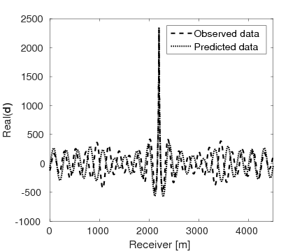
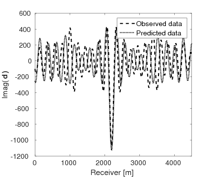
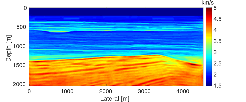
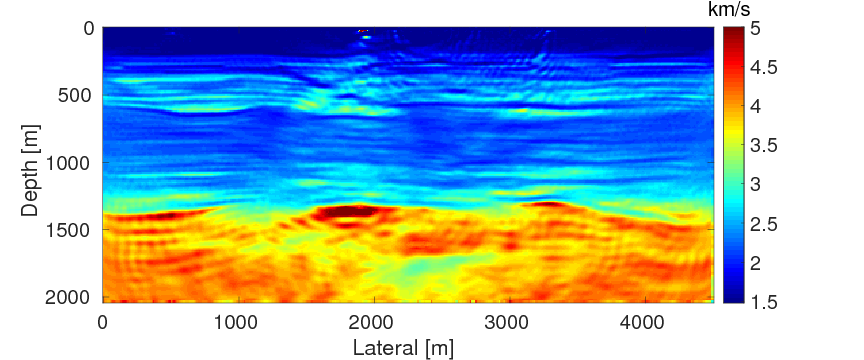
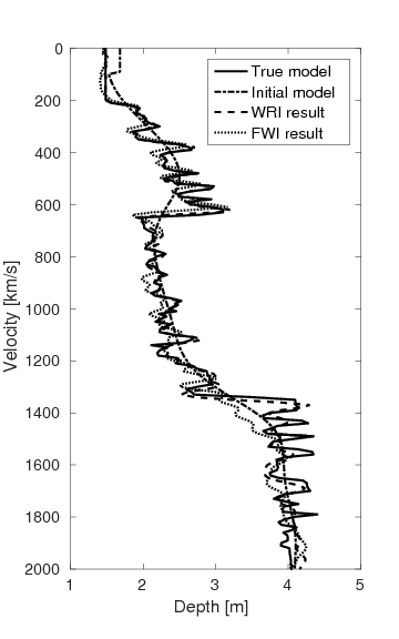
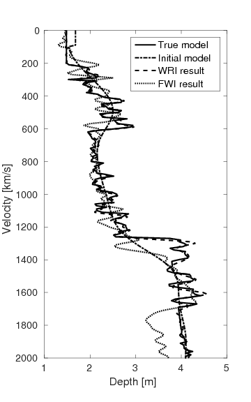
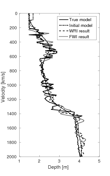
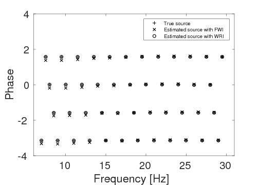
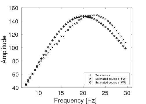
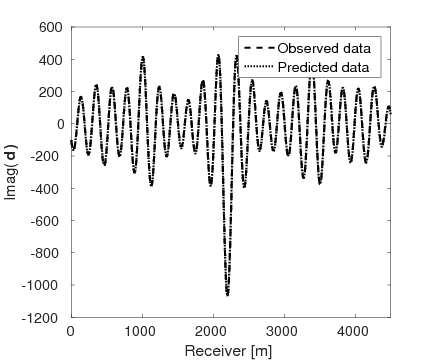
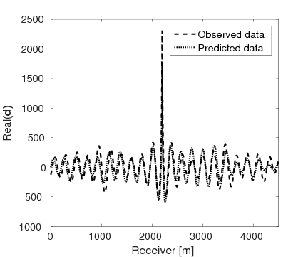
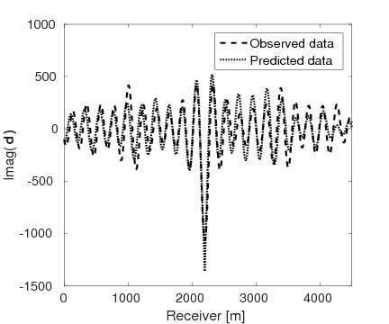
Figures 15a and 15b show the inversion results obtained by WRI and FWI, respectively. As expected, due to the cycle-skipped data and absence of low-frequency data, the conventional FWI fails to correctly invert the velocity in the shallow area where the transmitted waves arrive, i.e., \(z \, \leq \, 1.5 \, \mathrm{km}\), which subsequently yields larger errors within the inverted velocity in the deep part of the model, i.e., \(z \, > \, 1.5 \, \mathrm{km}\). On the other hand, WRI mitigates the negative effects of the cycle-skipped data to the inversion and correctly reconstructs the velocity in both areas that can and cannot be reached by the transmitted turning waves. The final average model error of WRI is \(0.1 \, \mathrm{km/s}\), which is much smaller than that of FWI—\(0.22 \, \mathrm{km/s}\). Moreover, as shown in Table 5, the \(\ell_2\)-norm model error of FWI is twice as large as that of WRI. This implies that besides the transmitted waves WRI also uses the reflection waves to invert the velocity model. Clearly, the main features and interfaces in the model are reconstructed correctly by WRI. Figure 16 displays three vertical cross-sections through the model. Compared to FWI, WRI provides a result that matches the true model much better. Figure 17 shows the comparison of the estimated source weights obtained by FWI and WRI. From the comparisons in Figures 17a and 17b, we observe that compared to FWI, WRI provides estimates of source weights with mildly better phases and significantly better amplitudes. The \(\ell_{2}\)-norm source error of FWI is much larger than that of WRI as shown in Table 5. This is not surprising as the quality of the source estimation and the inverted velocity model are closely tied to each other. Figure 18 shows the comparisons between the observed data and predicted data computed with the final results of WRI and FWI. The predicted data computed from the WRI inversion (Figures 18a and 18b) almost matches the observed data, while the mismatch of that from the FWI inversion is much larger (Figures 18c and 18d), which can also be found in the quantitative comparison in Table 5. All these results imply that besides providing a better velocity reconstruction, WRI also produces a better estimate of the source weights.
| FWI | WRI | |
|---|---|---|
| \(\|\mvec_{\text{t}}-\mvec_{\text{f}}\|_{2}\) | 100 | 50 |
| \(\|\alpha_{\text{t}}-\alpha_{\text{f}}\|_{2}\) | \(1.3e3\) | \(6e1\) |
| \(\|\d_{\text{obs}} - \d_{\text{pred}}\|_{2}\) | \(3.8e4\) | \(1.7e3\) |

Discussion
Source functions are essential for wave-equation-based inversion methods to conduct a successful reconstruction of the subsurface structures. Because the correct source functions are typically unavailable in practical applications, an on-the-fly source estimation procedure is necessary for the inversion. In this study, we proposed an on-the-fly source estimation technique for the recently developed WRI by adapting its variable projection procedure for the wavefields to include the source functions. Through simultaneously projecting out the wavefields and source functions, we obtained a reduced objective function that only depends on the medium parameters. As a result, we are able to accomplish the inversion without prior information of the source functions.
The main computational cost of the proposed source estimation method lies within the procedure of projecting out the wavefields and source weights, in which we have to invert a potentially ill-conditioned source-dependent matrix. For ocean bottom node and land acquisitions where all sources “see” the same receivers, we applied the block matrix inversion formula and arrived at a new inversion scheme that only involves inverting a source-independent matrix. This new scheme brings benefits to both direct and iterative solvers when compared to the direct inversion of the original source-dependent matrix. For 2D problems, we illustrated that without losing accuracy, the inversion of the proposed scheme only needs one Cholesky factorization for each frequency, while the direct inversion requires \(\nsrc\). Indeed, this benefit does not only apply to the Cholesky method, but also to other faster direct solvers including the multifrontal massively parallel sparse direct solver (MUMPS, Amestoy et al. (2016)), which can further speed up the projection procedure. When solving 3D problems with iterative solvers, the proposed inversion scheme reduces the number of preconditioners for each frequency from \(\nsrc\) to one; therefore, it significantly reduces the computational complexity. Furthermore, the source-independent matrix required to invert is the same one as in the conventional WRI without source estimation. Thus, we avoid iteratively inverting the potentially ill-conditioned source-dependent matrix and can straightforwardly apply any efficient and scalable methods designed for the conventional WRI (Peters et al., 2015) to the proposed approach, which allows us to extend the application of this approach to 3D frequency-domain waveform inversions.
Aside from benefiting inversions with ocean bottom node and land acquisitions, the proposed scheme may also benefit inversions with conventional 3D marine towed-streamer acquisitions where all sources “see” different receivers. In this case, we may lose the benefit of reducing the number of preconditioners due to the acquisition geometry, however, the benefit that avoids the direct inversion of the potentially ill-conditioned source-dependent matrix remains. As a result, we still can straightforwardly apply any preconditioners designed for the conventional WRI without source estimation to solve the proposed scheme. With carefully designed preconditioners, the computational cost of the proposed WRI with source estimation can be roughly equal to that of standard 3D frequency-domain FWI using iterative solvers, because the total numbers of the iterative PDE solves required by the two approaches are approximately the same. As a result, it should be viable to apply the proposed WRI with source estimation to inversions with the conventional 3D marine towed-streamer acquisitions.
While the presented examples illustrated the feasibility of the proposed approach—WRI with source estimation—for frequency-domain inversions, its extension to the time-domain inversions is not trivial. The main computational challenge lies in the fact that in the time domain, the projection procedure requires us to solve a very large linear system, whose size is \(n_{\text{time}}\) (number of time slices) times larger than that in the frequency domain. As a result, the computational and storage cost in the time domain is larger than that in the frequency domain. Moreover, the time-domain source function is a time series rather than a complex number in the frequency domain. In order to estimate the time series successfully, we may need additional constraints, such as the duration of the source function, to regularize the unknown source functions. Due to the two facts, the extension of the proposed approach to the time-domain inversions requires further investigations.
Conclusion
We showed that the recently proposed wavefield-reconstruction inversion method can be modified to handle unknown source situations. In the proposed modification of wavefield-reconstruction inversion, we considered the source weights as unknown variables and updated them jointly with the medium and wavefields parameters. To update the three unknowns, we proposed an optimization strategy based on the variable projection method. During each iteration of the inversion, for fixed medium parameters, the objective function is quadratic with respect to both wavefields and source weights. This fact motivates us to use the variable projection method to first project out the wavefields and source weights simultaneously, and then to update the medium parameters. As a result, we obtained an objective that does not depend on the wavefields and the source weights. Numerical experiments illustrated that equipped with the proposed source estimation method wavefield-reconstruction inversion can produce accurate inversion results without prior knowledge of the true source weights. Moreover, this method can also produce reliable results when the observations contain noise.
We also compared the proposed on-the-fly source estimation technique for wavefield-reconstruction inversion to the conventional source estimation technique for full-waveform inversion. The numerical result illustrated that by extending the search space and the inexact PDE-fitting, the proposed source estimation technique for wavefield-reconstruction inversion is less sensitive to inaccurate initial models and can start the inversion with data without low-frequency components.
Acknowledgments
We would like to acknowledge Charles Jones (BG Group) for providing the BG Compass model. This research was carried out as part of the SINBAD project with the support of the member organizations of the SINBAD Consortium.
Akcelik, V., 2002, Multiscale Newton-Krylov methods for inverse acoustic wave propagation: PhD thesis,. Carnegie Mellon University.
Amestoy, P., Brossier, R., Buttari, A., L’Excellent, J.-Y., Mary, T., Métivier, L., … Operto, S., 2016, Fast 3D frequency-domain full-waveform inversion with a parallel block low-rank multifrontal direct solver: Application to OBC data from the North Sea: Geophysics, 81(6), R363–R383.
Aravkin, A. Y., and van Leeuwen, T., 2012, Estimating nuisance parameters in inverse problems: Inverse Problems, 28, 115016. doi:10.1088/0266-5611/28/11/115016
Askan, A., Akcelik, V., Bielak, J., and Ghattas, O., 2007, Full waveform inversion for seismic velocity and anelastic losses in heterogeneous structures: Bulletin of the Seismological Society of America, 97, 1990–2008.
Bernstein, D. S., 2005, Matrix mathematics: Theory, facts, and formulas with application to linear systems theory: Princeton University Press Princeton.
Brossier, R., Operto, S., and Virieux, J., 2009, Seismic imaging of complex onshore structures by 2D elastic frequency-domain full-waveform inversion: Geophysics, 74(6), WCC105–WCC118.
Chen, Z., Cheng, D., Feng, W., and Wu, T., 2013, An optimal 9-point finite difference scheme for the Helmholtz equation with PML: International Journal of Numerical Analysis and Modeling, 10, 389–410.
Golub, G., and Pereyra, V., 2003, Separable nonlinear least squares: The variable projection method and its applications: Inverse Problems, 19, R1.
Huang, G., Symes, W., and Nammour, R., 2016, Matched source waveform inversion: Volume extension: 86th annual international meeting. SEG, Expanded Abstracts.
Li, M., Rickett, J., and Abubakar, A., 2013, Application of the variable projection scheme for frequency-domain full-waveform inversion: Geophysics, 78(6), R249–R257.
Li, X., Aravkin, A. Y., Leeuwen, T. van, and Herrmann, F. J., 2012, Fast randomized full-waveform inversion with compressive sensing: Geophysics, 77(3), A13–A17. doi:10.1190/geo2011-0410.1
Liu, J., Abubakar, A., Habashy, T., Alumbaugh, D., Nichols, E., and Gao, G., 2008, Nonlinear inversion approaches for cross-well electromagnetic data collected in cased-wells: 78th annual international meeting. SEG, Expanded Abstracts.
Nocedal, J., and Wright, S. J., 2006, Numerical optimization: Springer-Verlag New York. doi:10.1007/978-0-387-40065-5
Peters, B., and Herrmann, F. J., 2016, Constraints versus penalties for edge-preserving full-waveform inversion: The Leading Edge, 36, 94–100.
Peters, B., Greif, C., and Herrmann, F. J., 2015, An algorithm for solving least-squares problems with a Helmholtz block and multiple right-hand-sides: International conference on preconditioning techniques for scientific and industrial applications. Retrieved from https://www.slim.eos.ubc.ca/Publications/Private/Conferences/PRECON/2015/peters2015PRECONasl/peters2015PRECONasl_pres.pdf
Peters, B., Herrmann, F. J., and Leeuwen, T. van, 2014, Wave-equation based inversion with the penalty method: Adjoint-state versus wavefield-reconstruction inversion: 76th eAGE conference and exhibition 2014. EAGE. Retrieved from https://www.slim.eos.ubc.ca/Publications/Public/Conferences/EAGE/2014/peters2014EAGEweb.pdf
Plessix, R.-E., 2006, A review of the adjoint-state method for computing the gradient of a functional with geophysical applications: Geophysical Journal International, 167, 495–503.
Pratt, R. G., 1999, Seismic waveform inversion in the frequency domain, Part 1: Theory and verification in a physical scale model: Geophysics, 64, 888–901.
Symes, W. W., Sun, D., and Enriquez, M., 2011, From modelling to inversion: Designing a well-adapted simulator: Geophysical Prospecting, 59, 814–833.
Tarantola, A., and Valette, B., 1982, Generalized nonlinear inverse problems solved using the least squares criterion: Reviews of Geophysics, 20, 219–232. doi:10.1029/RG020i002p00219
van Leeuwen, T., and Herrmann, F. J., 2013, Fast Waveform Inversion without source-encoding: Geophysical Prospecting, 61, 10–19. Retrieved from http://dx.doi.org/10.1111/j.1365-2478.2012.01096.x
van Leeuwen, T., and Herrmann, F. J., 2015, A penalty method for PDE-constrained optimization in inverse problems: Inverse Problems, 32, 015007. Retrieved from https://www.slim.eos.ubc.ca/Publications/Public/Journals/InverseProblems/2015/vanleeuwen2015IPpmp/vanleeuwen2015IPpmp.pdf
van Leeuwen, T., and Herrmann, F. J., {2013}, Mitigating local minima in full-waveform inversion by expanding the search space: Geophysical Journal International, 195, 661–667. doi:10.1093/gji/ggt258
van Leeuwen, T., Aravkin, A. Y., and Herrmann, F. J., 2014, Comment on: Application of the variable projection scheme for frequency-domain full-waveform inversion (M. Li, J. Rickett, and A. Abubakar, Geophysics, 78, no. 6, R249R257): Geophysics, 79(3), X11–X17. doi:10.1190/geo2013-0466.1
Virieux, J., and Operto, S., 2009, An overview of full-waveform inversion in exploration geophysics: Geophysics, 74(6), WCC1–WCC26. doi:10.1190/1.3238367
Warner, M., Nangoo, T., Shah, N., Umpleby, A., Morgan, J., and others, 2013, Full-waveform inversion of cycle-skipped seismic data by frequency down-shifting: 83th annual international meeting. SEG, Expanded Abstracts.
Zhou, B., and Greenhalgh, S. A., 2003, Crosshole seismic inversion with normalized full-waveform amplitude data: Geophysics, 68, 1320–1330.