![]()
![]()
Abstract
Irregular or off-the-grid spatial sampling of sources and receivers is inevitable in field seismic acquisitions. Consequently, time-lapse surveys become particularly expensive since current practices aim to replicate densely sampled surveys for monitoring changes occurring in the reservoir due to hydrocarbon production. We demonstrate that under certain circumstances, high-quality prestack data can be obtained from cheap randomized subsampled measurements that are observed from nonreplicated surveys. We extend our time-jittered marine acquisition to time-lapse surveys by designing acquisition on irregular spatial grids that render simultaneous, subsampled and irregular measurements. Using the fact that different time-lapse data share information and that nonreplicated surveys add information when prestack data are recovered jointly, we recover periodic densely sampled and colocated prestack data by adapting the recovery method to incorporate a regularization operator that maps traces from an irregular spatial grid to a regular periodic grid. The recovery method is, therefore, a combined operation of regularization, interpolation (estimating missing fine-grid traces from subsampled coarse-grid data), and source separation (unraveling overlapping shot records). By relaxing the insistence on replicability between surveys, we find that recovery of the time-lapse difference shows little variability for realistic field scenarios of slightly nonreplicated surveys that suffer from unavoidable natural deviations in spatial sampling of shots (or receivers) and pragmatic compressed-sensing based nonreplicated surveys when compared to the “ideal” scenario of exact replicability between surveys. Moreover, the recovered densely sampled prestack baseline and monitor data improve significantly when the acquisitions are not replicated, and hence can serve as input to extract poststack attributes used to compute time-lapse differences. Our observations are based on experiments conducted for an ocean-bottom cable survey acquired with time-jittered continuous recording assuming source equalization (or same source signature) for the time-lapse surveys and no changes in wave heights, water column velocities or temperature and salinity profiles, etc.
This is part 2 of a two-paper series on time-lapse seismic with compressed sensing. Part 1: “Low-cost time-lapse seismic with distributed Compressive Sensing—exploiting common information among the vintages.” Authors: Felix Oghenekohwo, Haneet Wason, Ernie Esser, and Felix J. Herrmann.
Introduction
Simultaneous marine acquisition is being recognized as an economic and environmentally more sustainable way to sample seismic data and speedup acquisition, wherein single or multiple source vessels fire shots at random, compressed times resulting in overlapping shot records (Kok and Gillespie, 2002; Beasley, 2008; Berkhout, 2008; Hampson et al., 2008; Moldoveanu and Quigley, 2011; Abma et al., 2013), and hence generating compressed seismic data volumes. The aim then is to separate the overlapping shot records into individual shot records, as acquired during conventional acquisition, but with denser source sampling while preserving amplitudes of the late, often weak, arrivals. This leads to recovering densely sampled data economically, which is essential for producing high-resolution images of the subsurface.
Mansour et al. (2012), Wason and Herrmann (2013) and C. Mosher et al. (2014) have showed that compressed sensing (CS, Candès et al., 2006b; D. L. Donoho, 2006) is a viable technology to sample seismic data economically with low environmental imprint—by reducing numbers of shots (or injected energy in the subsurface) or compressing survey times. Mansour et al. (2012) and Wason and Herrmann (2013) proposed an alternate sampling strategy for simultaneous acquisition (“time-jittered” marine), addressing the separation problem through a combination of tailored (simultaneous) acquisition design and sparsity-promoting recovery via convex optimization using \(\ell_1\) objectives. This separation technique interpolates sub-Nyquist jittered shot positions to a fine regular grid while unraveling the overlapping shots. The time-jittered marine acquisition is designed for continuous recording, fixed-receiver (or “static”) geometries, which is different from the case of towed-streamer (or “dynamic”) geometries, wherein multiple sources fire shots within a time interval of \((0,1)\) or \((0,2)\,\mathrm{s}\) generating overlapping shot records that need to be separated into its constituent sources, i.e., a data volume for each individual source (Kumar et al., 2015). Our approach for conventional data recovery from simultaneous data from static geometries can equally apply to other settings including static land and other static marine geometries.
The implications of randomization in time-lapse (or 4D) seismic, however, are less well-understood since the current paradigm relies on dense sampling and replicability amongst the baseline and monitor surveys (Lumley and Behrens, 1998). These requirements impose major challenges because the insistence on dense sampling may be prohibitively expensive and variations in acquisition geometries (between the surveys) due to physical constraints do not allow for exact replication of the surveys. In paper 1, we presented a new approach (the “joint recovery method”) that addresses these acquisition- and processing-related issues by explicitly exploiting common information shared by the different time-lapse vintages. Our analyses were carried out assuming that the observations lied on a discrete grid so that exact survey replicability is in principle achievable. We also assume sources to have the same source signature for the time-lapse surveys. While assuming source equalization in this paper, we extend our work on simultaneous time-jittered marine acquisition to time-lapse surveys for more realistic field acquisitions that lie on irregular spatial grids, where the notion of exact replicability of the surveys is inexistent. This is because the “real” world suffers from unavoidable deviations between pre- and post-acquisition shot (and receiver) positions, rendering regular, periodic spatial grids irregular, and hence exact replication of the surveys impossible. As mentioned later in the paper, accounting for the irregularity of seismic data is key to recovering densely sampled data. Moreover, while we do not insist that we actually visit predesigned (irregular) shot positions, but it is important to know these positions to sufficient accuracy after acquisition for high-quality data recovery. Recent successes in the application of compressed sensing to land and marine field data acquisition (see e.g., C. Mosher et al., 2014) show that this can be achieved in practice.
Simultaneous time-jittered marine acquisition generates compressed and subsampled data volumes, therefore, extending this to time-lapse surveys generates compressed and subsampled baseline and monitor data. Consequently, we are interested in recovering densely sampled vintages and time-lapse difference. Moreover, time-lapse differences are often studied via differences in certain poststack attributes computed from the vintages (Landrø, 2001; Spetzler and Kvam, 2006), hence, we prioritize on recovering the prestack vintages. In this paper, we push this technology to realistic settings of off-the-grid acquisitions and demonstrate that we actually gain if we relax the insistence to replicate surveys since even the smallest known deviations from the grid can lead to significant improvements in the recovery of the vintages with minimal compromise with the recovery of the time-lapse difference.
Motivation: on-the-grid vs. off-the-grid data recovery
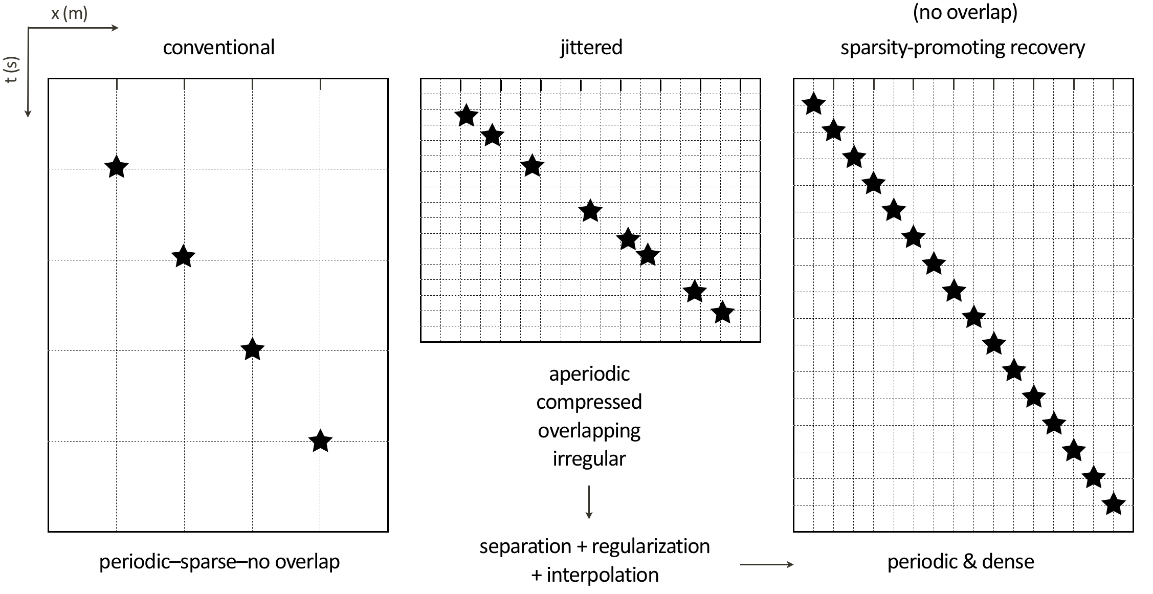
Paper 1 illustrated that the joint recovery method gives better recoveries of time-lapse data and time-lapse difference than the independent recovery strategy, since the former approach exploits the common information shared by the vintages. It also showed that “exact” replication of the baseline and monitor surveys lead to good recovery of the time-lapse difference but not of the vintages. These analyses, however, were carried out assuming that the observations lied on a discrete grid so that exact survey replicability is achievable. Realistic field acquisitions, on the contrary, lie off the grid—i.e., have irregular spatial sampling—where exact replicability of the surveys is inexistent. Figure 1 shows a comparison between conventional periodic acquisition which generates data with nonoverlapping shot records, and simultaneous time-jittered acquisition which generates compressed recordings with overlapping shots. Note that the sampling grid for conventional acquisition “in the field” would be slightly irregular, however, this in contrast to the jittered acquisition which by virtue of its design is aperiodic and lies on an irregular sampling grid. Since the time-jittered acquisition scheme leverages compressed sensing—the success of which hinges on randomized subsampling—additional and unavoidable deviations in the field add to the randomization of the designed irregular shot positions, and helps in sparsity-promoting inversion as long as we know the final shot positions to sufficient precision.
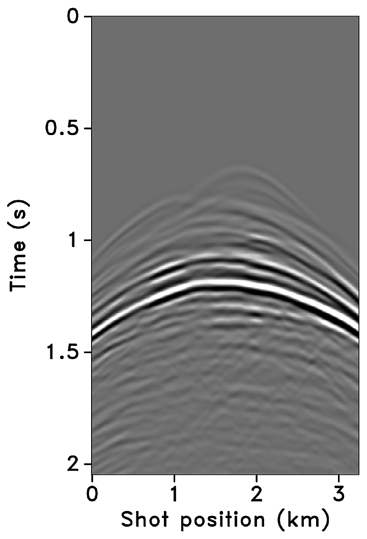
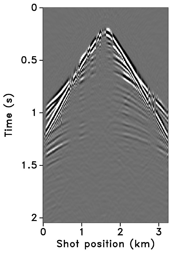
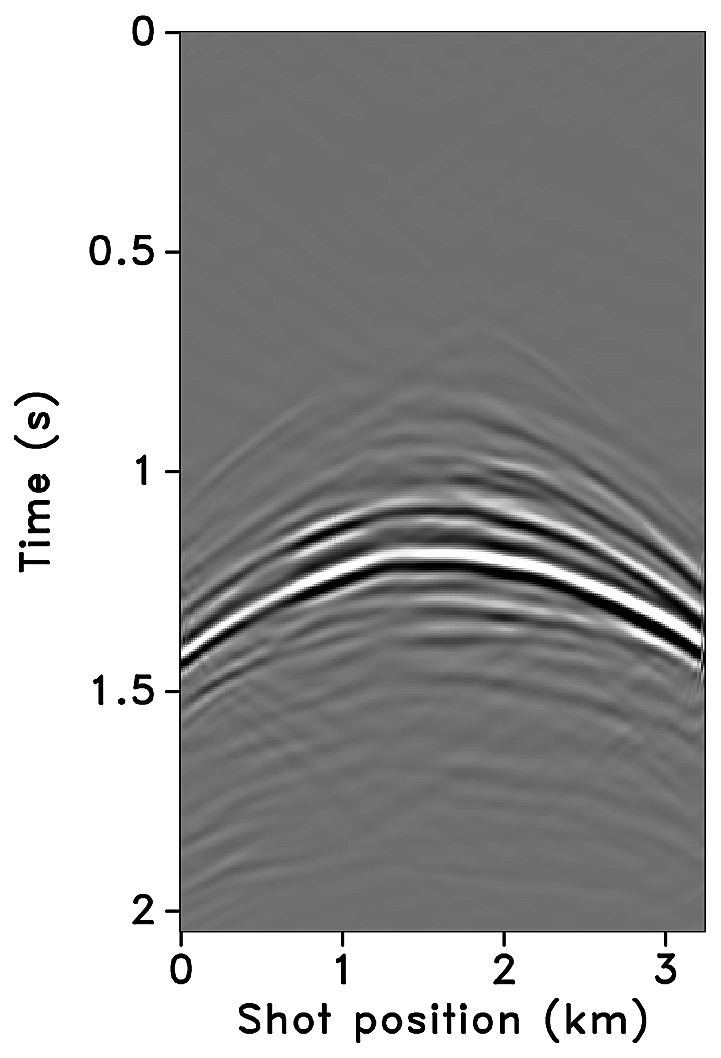
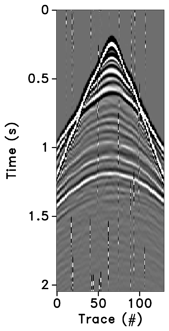
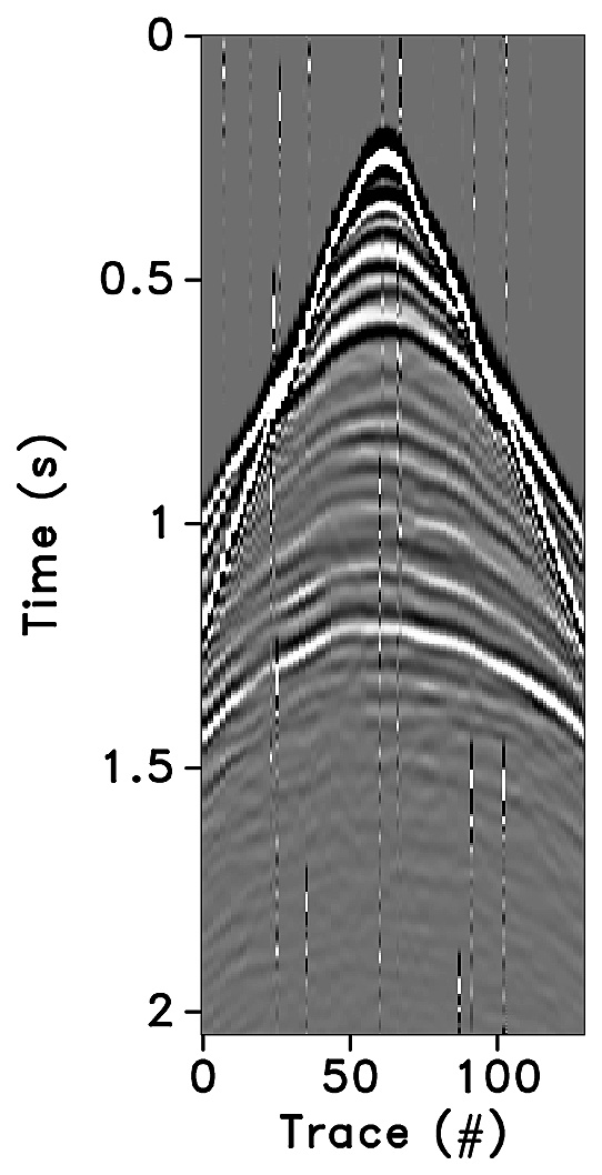
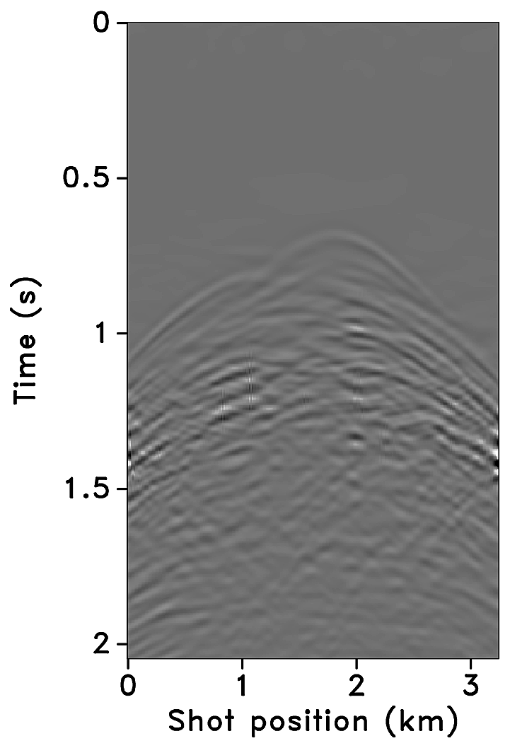
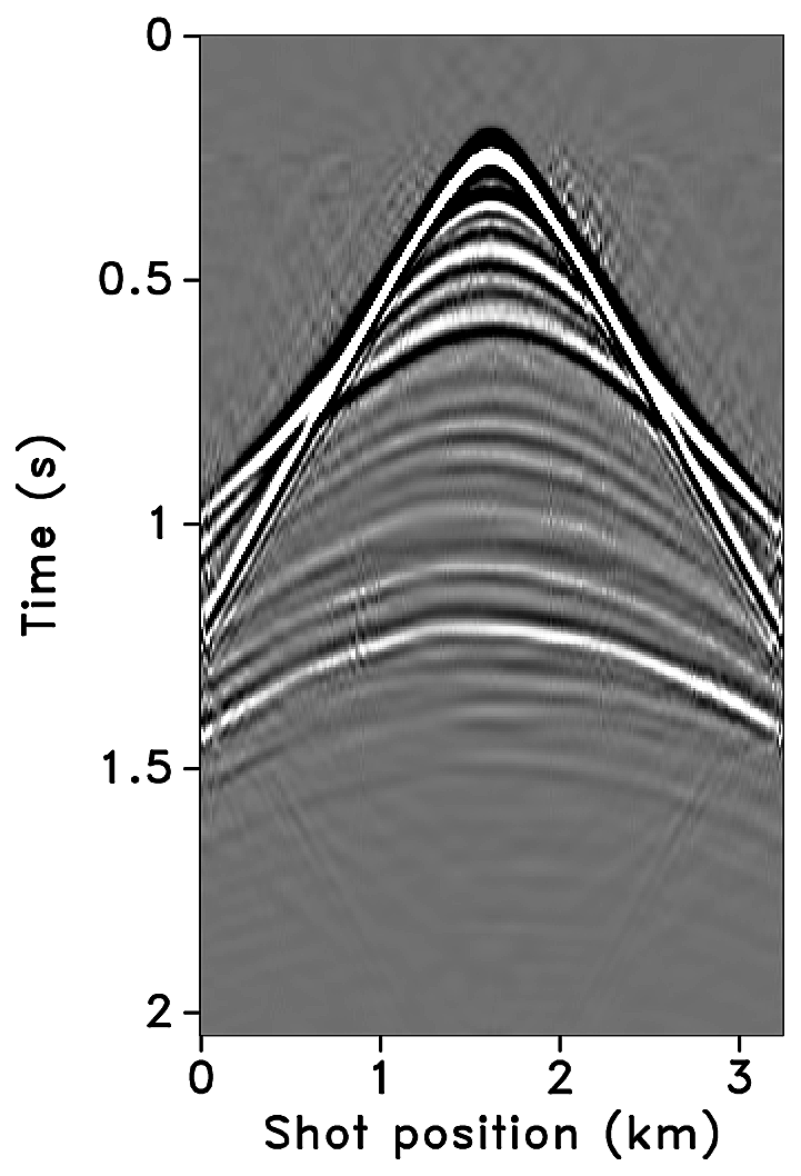
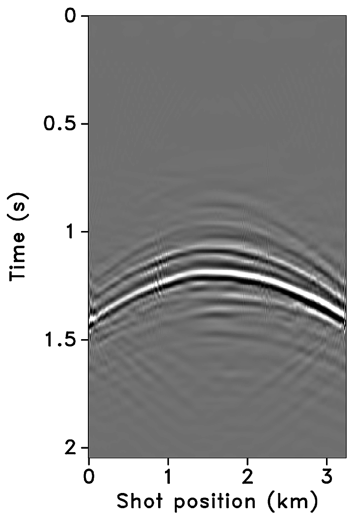
Figures 2a-2c show receiver gathers from a conventional (synthetic) time-lapse data set and the corresponding time-lapse difference. To recover periodic densely sampled data from simultaneous, compressed and irregular data, we could implicitly rely on binning, however, failure to account for irregularity of seismic traces can adversely affect the recovery as shown in Figure 3. This is because binning does not represent accurate positions of irregular traces. Note that this example corresponds to a time-jittered acquisition scheme for the baseline that is exactly replicated for the monitor. The results show that binning offsets all the gains of exact survey replication and also of the joint recovery method. Figure 4 illustrates the importance of regularization of irregular traces for high-quality data recovery. In this paper, therefore, we extend our work on simultaneous time-jittered acquisition to time-lapse surveys by acknowledging the irregularity of field seismic data and incorporating sparsifying transforms that exploit this irregularity to recover periodic densely sampled time-lapse data.


Contributions
The contributions of this work can be summarized as follows. First, we present an extension of our simultaneous time-jittered marine acquisition for time-lapse surveys by working on more realistic field acquisition scenarios by incorporating irregular spatial grids. Second, we leverage ideas from compressed sensing and distributed compressed sensing to develop an algorithm that separates simultaneous data, regularizes irregular traces and interpolates missing traces—all at once. Third, through simulated experiments, we show that insistence on replicability of time-lapse surveys can be relaxed since small known deviations in shot positions from a regular grid (or deviations in shot positions of the monitor survey from those in the baseline survey) lead to significant improvements in the recovery of the vintages, without drastic modifications in the recovery of the time-lapse difference.
Outline
The paper is organized as follows. We begin with the description of the simultaneous time-jittered marine acquisition design, where we explain how subsampled and irregular measurements are generated. Next, we introduce the nonequispaced fast discrete curvelet transform (NFDCT) and its application to recover periodic densely sampled seismic lines from simultaneous and irregular measurements via sparsity-promoting inversion. We then extend this framework to time-lapse surveys where we modify the measurement matrices in the joint recovery method to include the off-the-grid information—i.e., the irregular shot positions and jittered times. Note that we do not describe the independent recovery strategy since it is clear in paper 1 that the joint recovery method outperforms the former approach. We conduct a series of synthetic seismic experiments with different random realizations of the simultaneous time-jittered marine acquisition to assess the effects (or risks) of irregular sampling in the field on time-lapse data and demonstrate that high-quality data recoveries are the norm and not the exception. We show this by generating 2D seismic lines using two different velocity models—one with simple geology and complex time-lapse difference (BG COMPASS model), and the other with complex geology and complex time-lapse difference (SEAM Phase 1 model with simulated time-lapse difference). Aside from computing signal-to-noise ratios measured with respect to densely sampled true baseline, monitor, and time-lapse differences, we also measure the economic and environmental performance of the proposed acquisition design and recovery strategy by computing the improvement in spatial sampling.
Time-jittered marine acquisition
The objective of CS is to recover densely sampled data from (randomly) subsampled data by exploiting sparse structure in the data during sparsity-promoting recovery. Mansour et al. (2012), Wason and Herrmann (2013) presented a pragmatic simultaneous marine acquisition scheme, termed as time-jittered marine, that leverages ideas from compressed sensing by invoking randomness and subsampling—i.e., sample randomly with fewer samples than required by Nyquist sampling criteria in the acquisition via random jittering of the source firing times. The success of CS hinges on randomized subsampling since it renders subsampling related artifacts incoherent, and therefore nonsparse, favouring data recovery via structure-promoting inversion. Consequently, source interferences (in simultaneous acquisition) become incoherent in common-receiver gathers creating a favorable condition for separating simultaneous data into conventional nonsimultaneous data via curvelet-domain sparsity promotion. The CS paradigm, however, assumes signals to be sampled on a periodic discrete grid—i.e., signals with sparse representation in finite discrete dictionaries.
Data volumes collected during seismic acquisition represent discretization of analog finite-energy wavefields in up to five dimensions including time—i.e., we acquire an analog spatiotemporal wavefield \(\bar{f}(t,x) \in {L^2}((0,T] \times [-X,X]^4)\), two dimensions for receivers and two dimensions for sources, with time \(T\) in order of seconds and length \(X\) in order of kilometers. In an ideal world, signals would perfectly lie on a periodic, regular grid. Hence, with a linear high-resolution analog-to-digital converter \(\bar{\Phi_s}\), the discrete signal is represented as \(f[q] = \bar{f} \star \bar{\Phi_s}(q)\), for \(0 \leq q < N\) (Mallat, 2008), where the samples lie on a grid. Typically, these samples are organized into a vector \(\vector{f} = {f[q]}_{q=0,...,N-1} \in \mathbb{R}^N\). Signals we encounter in the real world, however, are usually not uniformly regular and do not lie on a regular grid. Therefore, it is imperative to define an irregular sampling adapted to the local signal regularity (Mallat, 2008). For irregular sampling, the discretized irregular signal is represented as \(f[q_n] = \bar{f} \star \bar{\Phi_s}(q_n)\), for \(n = 0, ..., M-1\) and \(M \leq N\), where \(q_n\) are irregular points (or nonequispaced nodes) randomly chosen from the set {\(0, ..., N-1\)}. Its vector representation is \(\vector{f} = {f[q_n]}_{n=0,...,M-1}\).
For a signal \(\vector{f}_0 \in \mathbb{R}^N\) that admits a sparse representation \(\vector{x}_0\) in some transform domain—i.e., \(\vector{f}_0\) is sparse with respect to a basis or redundant frame \(\vector{S} \in \mathbb{C}^{P \times N}\), with \(P \geq N\), such that \(\vector{f}_0 = \vector{S}^{H} \vector{x}_0\) (\(\vector{x}_0\) sparse), where \(^H\) denotes the Hermitian transpose—the goal in CS is to reconstruct the signal \(\vector{f}_0\) from few random linear measurements, \(\vector{y} = \vector{Af}_0\), where \(\vector{A}\) is an \(n \times N\) measurement matrix with \(n \ll N\). Utilizing prior knowledge that \(\vector{f}_0\) is sparse with respect to a basis or redundant frame \(\vector{S}\) and assuming the signal to be sampled on a periodic discrete grid, CS aims to find an estimate \(\tilde{\vector{x}}\) for the underdetermined system of linear equations: \(\vector{y} = \vector{Af}_0\). This is done by solving the basis pursuit (BP, Candès et al., 2006b; D. L. Donoho, 2006) convex optimization problem: \[ \begin{equation} \tilde{\vector{x}} = \argmin_{\vector{x}}\|\vector{x}\|_1\DE\sum_{i=1}^N|x_i| \quad \text{subject to} \quad \vector{y} = \vector{Ax}. \label{eqBP} \end{equation} \] In the noise-free case, this problem finds amongst all possible vectors \(\vector{x}\), the vector that has the smallest \(\ell_1\)-norm and that explains the observed subsampled data.
Mathematically, a seismic line with \(N_s\) sources, \(N_r\) receivers, and \(N_t\) time samples can be reshaped into an \(N\) dimensional vector \(\vector{f}\), where \(N = N_s \times N_r \times N_t\). Since real-world signals are not exactly sparse but compressible—i.e., can be well approximated by a sparse signal—a compressible representation, \(\vector{x}\), of the seismic line in the curvelet domain, \(\vector{S}\), is represented as \(\vector{f} = \vector{S}^H \vector{x}\). Since curvelets are a redundant frame (an over-complete sparsifying dictionary), \(\vector{S} \in \mathbb{C}^{P \times N}\) with \(P > N\), and \(\vector{x} \in \mathbb{C}^P\). With the inclusion of the sparsifying transform, the measurement matrix \(\vector{A}\) can be factored into the product of a \(n \times N\) (with \(n \ll N\)) acquisition matrix \(\vector{M}\) and the synthesis matrix \(\vector{S}^H\)—i.e., \(\vector{A} = \vector{MS}^H\). For the real-world irregular signals, however, we need to account for the acquired unstructured measurements for high-resolution data recovery. We do this by introducing an operator in the recovery algorithm (by modifying the measurement operator \(\vector{A}\)—see details in the next sections) that acknowledges the irregularity of seismic traces and uses this information to render regularized and interpolated data.
Acquisition geometry
In time-jittered marine acquisition, source vessels map the survey area firing shots at jittered time instances, which translate to jittered shot positions for a given (fixed) speed of the source vessel. The simultaneous data is time compressed, and therefore acquired economically with low environmental imprint. The recovered separated data is periodic and dense. For simplicity, we assume that all shot positions see the same receivers, which makes our method applicable to marine acquisition with ocean bottom cables or nodes (OBC or OBN). The receivers record continuously resulting in simultaneous shot records. Randomization via jittered subsampling offers control over the maximum gap size (on the acquisition grid), which is a practical requirement of wavefield reconstruction with localized sparsifying transforms such as curvelets (Hennenfent and Herrmann, 2008). For simultaneous time-jittered acquisition, parameters such as the minimum distance required between adjacent shots and minimum recharge time for the air guns help in controlling the maximum acquisition gap while maintaining the minimum realistic acquisition gap.
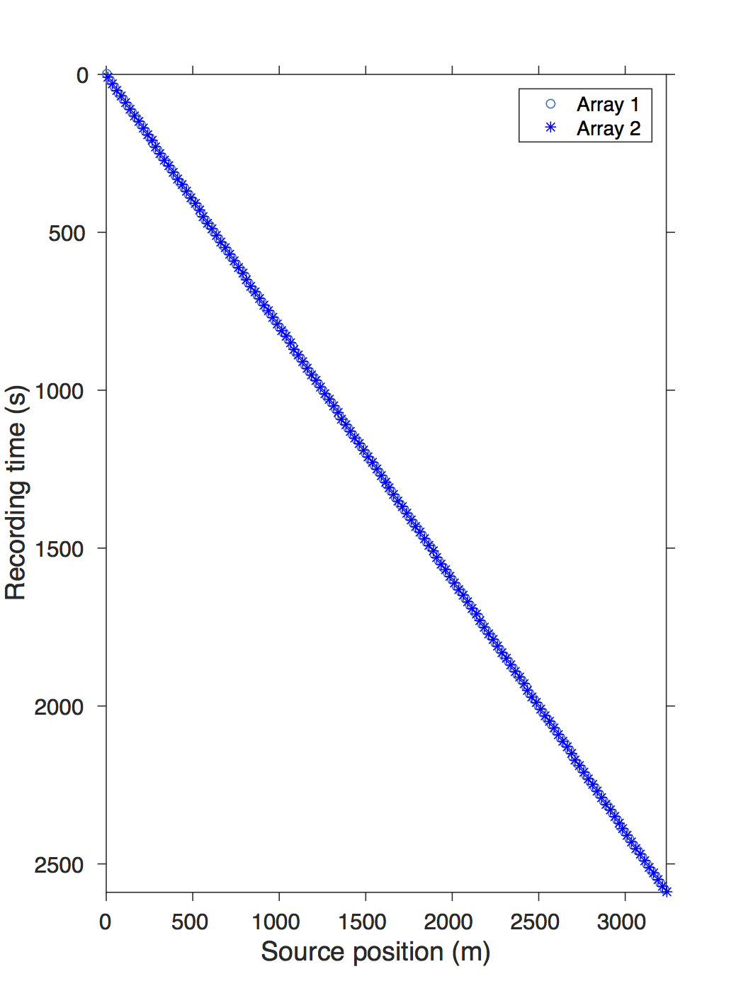
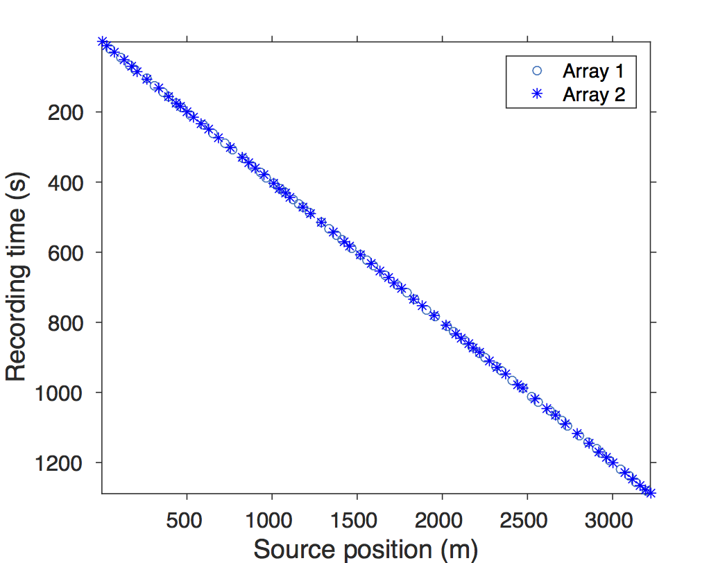
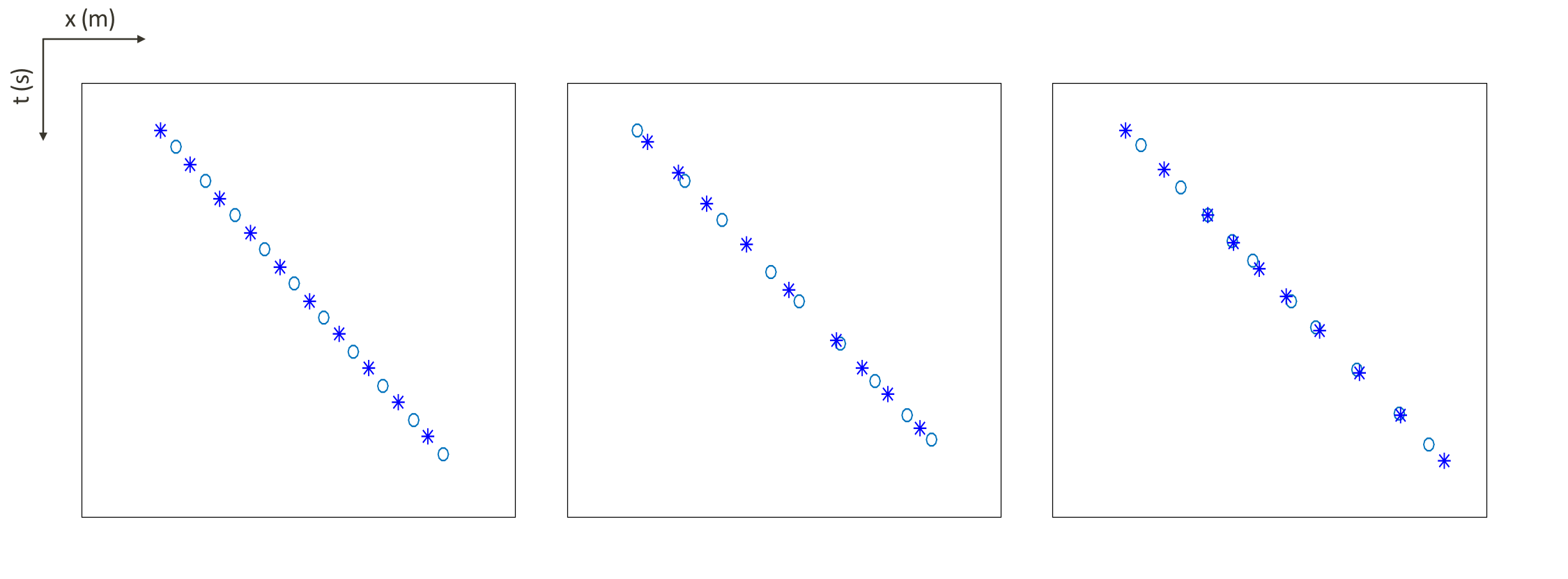
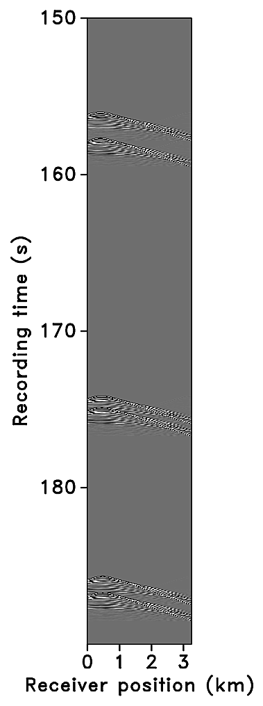
Conventional acquisition with one source vessel and two air-gun arrays where each air-gun array fires at every alternate periodic location is called flip-flop acquisition. If we wish to acquire \(10.0\, \mathrm{s}\)-long shot records at every \(12.5\,\mathrm{m}\), the speed of the source vessel would have to be about \(1.25\,\mathrm{m/s}\) (\(\approx 2.5\) knots). Figure 5a illustrates one such conventional acquisition scheme, where each air-gun array fires every \(20.0\,\mathrm{s}\) (or \(25.0\,\mathrm{m}\)) in a flip-flop manner traveling at about \(1.25\,\mathrm{m/s}\), resulting in nonoverlapping shot records of \(10.0\,\mathrm{s}\) every \(12.5\,\mathrm{m}\). In time-jittered acquisition, Figures 5b and 5c, each air-gun array fires on average at every \(20.0\,\mathrm{s}\) jittered time-instances traveling at about \(2.5\,\mathrm{m/s}\) (\(\approx 5.0\) knots) with the receivers (OBC/OBN) recording continuously, resulting in overlapping shot records (Figures 6a and 6b). Note that the acquisition design involves jittered subsampling—i.e., regular decimation of the (fine) interpolation grid and subsequent perturbation of the coarse-grid points completely off the fine grid. The idealized discrete jittered subsampling, by contrast, perturbs the coarse-grid points on the fine grid, as presented in paper 1. The subsampling factor is represented by \(\eta\). Therefore, the acquired data volume has overlapping shots and missing shots/traces (Figure 6a and 6b). For this reason, the jittered flip-flop acquisition might not mimic the conventional flip-flop acquisition where air-gun array 1 and 2 fire one after the other—i.e., in the center and right-hand plots of Figure 5d a circle (denoting array 1) may be followed by another circle instead of a star (denoting array 2), and vice versa. However, the minimum interval between the jittered times is maintained at \(10.0\,\mathrm{s}\) (typical interval required for air-gun recharge), while the maximum interval is \(30.0\,\mathrm{s}\). For the speed of \(2.5\,\mathrm{m/s}\), this translates to jittering a \(50.0\,\mathrm{m}\) source grid with a minimum (and maximum) interval of \(25.0\,\mathrm{m}\) (and \(75.0\,\mathrm{m}\)) between jittered shots. Both arrays fire at the \(50.0\,\mathrm{m}\) jittered grid independent of each other.

In time-jittered marine acquisition, the acquisition operator \(\vector{M}\) is a combined jittered-shot selector and time-shifting operator. Since data is acquired on an irregular grid, it is imperative to incorporate operators in the design of the acquisition matrix \(\vector{M}\) that account for and hence regularize the irregularity in the data. This is critical to the success of the recovery algorithm. The off-the-grid acquisition design is different from that presented by Li et al. (2012), wherein an interpolated restriction operator accounts for irregular points by incorporating Lagrange interpolation into the restriction operator—i.e., the measurements are approximated using a \(k^{\text{th}}\)-order Lagrange interpolation. In time-jittered acquisition, the jittered time instances are put on a time grid (defined by a time-sampling interval) where each jittered time instance is placed on the point closest to it on the regular time grid. The difference between the true jittered time and the regular grid point, \(\Delta{t}\), is corrected by shifting the traces by \(e^{-i\omega\Delta{t}}\), where \(\omega\) is the angular frequency. The irregularity in the shot positions is corrected by including the nonequispaced fast Fourier transform, NFFT (Potts et al., 2001; Kunis, 2006), in the sparsifying operator \(\vector{S}\) (Hennenfent and Herrmann, 2006; Hennenfent et al., 2010), as described in the next section. The NFFT evaluates a Fourier expansion at nonequispaced locations defined by the time-jittered acquisition. Note that in this framework it is also possible to randomly subsample the receivers.
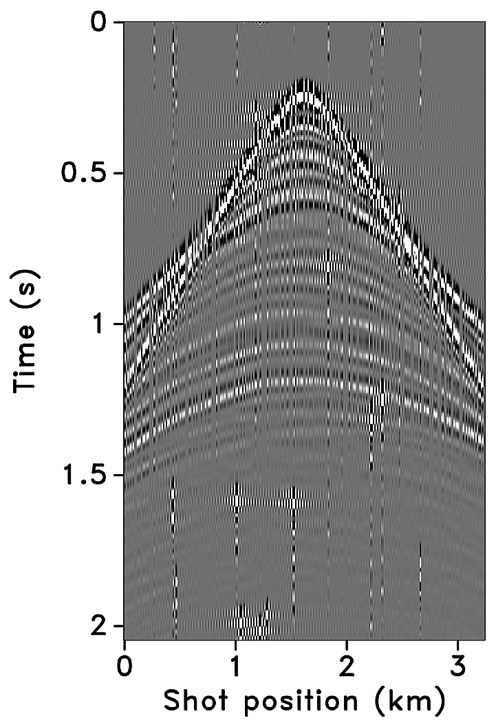
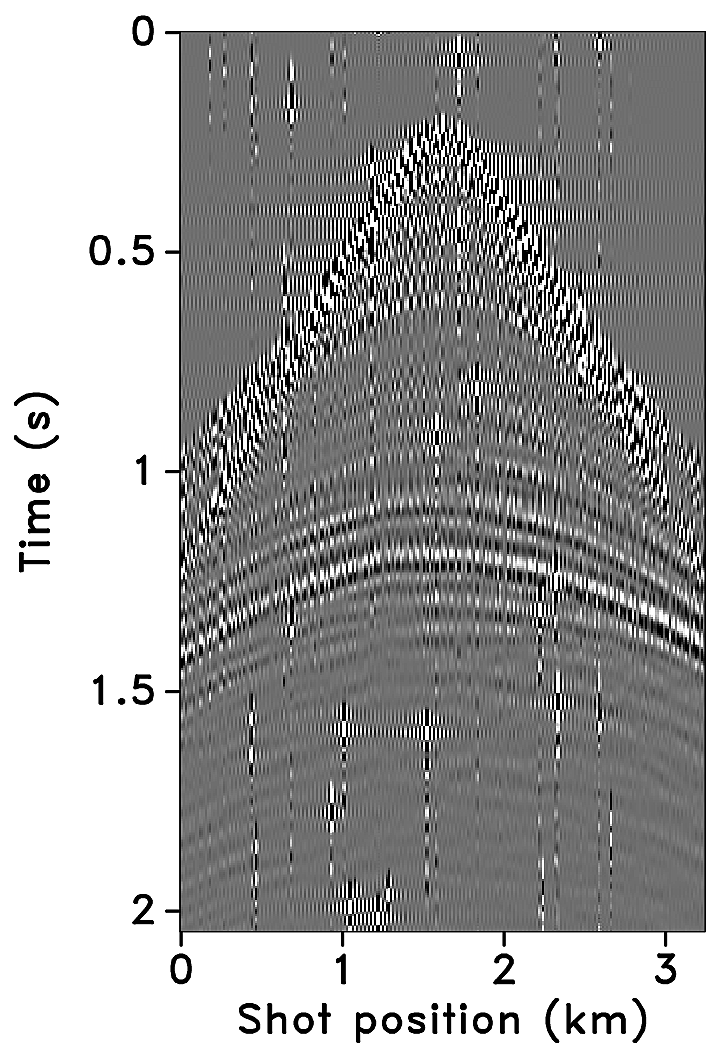
Randomly subsampled and simultaneous measurements for the baseline and monitor surveys are shown in Figures 6a and 6b, respectively. Note that only \(40.0\,\mathrm{s}\) of the continuously recorded data is shown. If we simply apply the adjoint of the acquisition operator to the corresponding simultaneous data—i.e., \(\vector{M}^H\vector{y}\)—the interferences (or source crosstalk) due to overlapping shots appear as incoherent and nonsparse in the receiver gathers (Figures 7a and 7b). Moreover, since regularization (and interpolation) is performed by the NFFT inside a nonequispaced curvelet framework (see next section), Figures 7a and 7b have \(\frac{N_s}{\eta}\) irregular traces, where \(\eta > 1\) is the subsampling factor. Since the baseline and monitor surveys have different irregular shot positions, the corresponding time-lapse difference cannot be computed unless both time-lapse data are realigned to a common spatal grid. For this purpose, if we apply the adjoint of a 1D NFFT operator \(\vector{N}\)—i.e., \(\vector{N}^H\vector{M}^H\vector{y}\)—the time-lapse data are realigned to a common fine spatial grid (Figures 7c and 7d). The corresponding time-lapse difference is shown in Figure 7e. As illustrated by these figures, in order to eventually remove the interferences and interpolate missing traces it is important to consider the recovery problem as an inversion problem. Since the time-jittered acquisition generates simultaneous, irregular data with missing traces, the recovery problem becomes a joint source separation, regularization and interpolation problem.


From discrete to continuous spatial subsampling
Subsampling schemes that are based on an underlying fine interpolation grid incorporate the discrete (spatial) subsampling schemes, since the subsampling is done on the grid. This situation typically occurs when binning continuous randomly-sampled seismic data into small bins that define the fine grid used for interpolation (Hennenfent and Herrmann, 2008). For such cases, the wrapping-based fast discrete curvelet transform, FDCT via wrapping (Candès et al., 2006a) can be used to recover the fully sampled data since the inherent fast Fourier transform (FFT) assumes regular sampling along all coordinates. For the interested reader, the curvelet transform is a multiscale, multidirectional, and localized transform that corresponds to a specific tiling of the f-k domain into dyadic annuli based on concentric squares centered around the zero-frequency zero-wavenumber point. Each annulus is subdivided into parabolic angular wedges—i.e., length of wedge \(\propto\) width\(^2\) of wedge. The architecture of the analysis operator (or forward operation) of the FDCT via wrapping is as follows: (1) apply the analysis 2D FFT; (2) form the angular wedges; (3) wrap each wedge around the origin; and (4) apply the synthesis 2D FFT to each wedge. The synthesis/adjoint operator—also the inverse owing to the tight-frame property—is computed by reversing these operations (Candès et al., 2006a).
Seismic data, however, is usually acquired irregularly, typically nonuniformly sampled along the spatial coordinates. Simultaneous time-jittered marine acquisition, mentioned above, is an instance of acquiring seismic data on irregular spatial grids. Hence, binning can lead to a poorly-jittered subsampling scheme, which will not favor wavefield reconstruction by sparsity-promoting inversion. Moreover, failure to account for the nonuniformly sampled data can adversely affect seismic processing, imaging, etc. Therefore, we should work with an extension to the curvelet transform for irregular grids (Hennenfent et al., 2010). Using this extension for the simultaneous time-jittered marine acquisition will produce colocated fine-scale time-lapse data. Continuous random sampling typically leads to improved interpolation results because it does not create coherent subsampling artifacts (Xu et al., 2005).
Nonequispaced fast discrete curvelet transform (NFDCT)
For irregularly acquired seismic data, the (FFT inside) FDCT (Candès et al., 2006a) assumes regular sampling along all (spatial) coordinates. Ignoring the nonuniformity of the spatial sampling no longer helps in detecting the wavefronts because of a lack of continuity. Hennenfent and Herrmann (2006) addressed this issue by extending the FDCT to nonuniform (or irregular) grids via the nonequispaced fast Fourier transform, NFFT (Potts et al., 2001; Kunis, 2006). The outcome was the ‘first generation NFDCT’ (nonequispaced fast discrete curvelet transform), which relied on accurate Fourier coefficients obtained by an \(\ell_{2}\)-regularized inversion of the NFFT.
The NFDCT handles irregular sampling, thus, exploring continuity along the wavefronts by viewing seismic data in a geometrically correct way—typically nonuniformly sampled along the spatial coordinates (source and/or receiver). In Hennenfent et al. (2010), the authors introduced a ‘second generation NFDCT’, which is based on a direct, \(\ell_{1}\)-regularized inversion of the operator that links curvelet coefficients to irregular data. Unlike the first generation NFDCT, the second generation NFDCT is lossless by construction—i.e., the curvelet coefficients explain the data at irregular locations exactly. This property is important for processing irregularly sampled seismic data in the curvelet domain and bringing them back to their irregular recording locations with high fidelity. Note that the second generation NFDCT is lossless for regularization not interpolation. The NFDCT framework as setup in Hennenfent et al. (2010) basically involves a Kronecker product (\(\otimes\)) of a 1D FFT operator \(\vector{F}_{t}\), used along the temporal coordinate, and a 1D NFFT operator \(\vector{N}_{x}\), used along the spatial coordinate, followed by the application of the curvelet tilling operator \(\vector{T}\) that maps curvelet coefficients to the Fourier domain—i.e., \(\vector{B}\;{\buildrel\rm def\over=}\;\vector{T} (\vector{N}_x \otimes \vector{F}_t)\). Therefore, \(\vector{B}\) is the NFDCT operator that links the curvelet coefficients to nonequispaced traces. The 1D NFFT operator (\(\vector{N}_{x}\)) replaces the 1D FFT operator (\(\vector{F}_{x}\)) that acts along the spatial coordinate in FDCT. Note that the NFDCT operator described above is written differently than in Hennenfent et al. (2010) because the latter defines the synthesis FFT operator as \(\vector{F}\), whereas \(\vector{F}\) is the analysis FFT operator in this paper. This also ensures consistency of notation and terminology with paper 1.
For the proposed simultaneous acquisition, the joint problem of source separation, regularization and interpolation is addressed by using a sparsifying operator (\(\vector{S}\)) that handles the multidimensionality of this problem. Therefore, \(\vector{S}\;{\buildrel\rm def\over=}\;\vector{C} \otimes \vector{W}\), where \(\vector{C}\) is a 2D NFDCT operator and \(\vector{W}\) is a 1D wavelet operator. The NFDCT operator is modified as \[ \begin{equation} \vector{C}\;{\buildrel\rm def\over=}\;\vector{T} (\vector{N}_{xs} \otimes \vector{F}_{xr}), \label{eqmodNFDCT} \end{equation} \] where the 1D NFFT operator \(\vector{N}_{xs}\) acts along the jittered shot coordinate and the 1D FFT operator \(\vector{F}_{xr}\) acts along the regular receiver coordinate. The 1D wavelet operator is applied on the time coordinate. As mentioned previously, the measurement matrix \(\vector{A} = \vector{MS}^H\). From a practical point of view, it is important to note that matrix-vector products with all the matrices are matrix free—i.e., these matrices are operators that define the action of the matrix on a vector, but are never formed explicitly.
In summary, recovery of nonoverlapping, periodic and densely sampled data from simultaneous, irregular and compressed data is achieved by incorporating an NFFT operator inside the curvelet framework that acts along the irregular spatial coordinate(s) and applying time shifts to the traces wherever necessary. Note that the NFFT operator is incorporated in the 2D NFDCT operator \(\vector{C}\), which is incorporated in the sparsifying operator \(\vector{S}\), and the time shift \(\Delta{t}\) is incorporated in the acquisition operator \(\vector{M}\). The NFFT computes (fine grid) 2D Fourier coefficients by mapping the coarse nonuniform spatial grid to a fine uniform grid. The curvelet coefficients are computed directly from the 2D Fourier coefficients.
Time-lapse acquisition via jittered sources
In paper 1, we extended the time-jittered marine acquisition to time-lapse surveys where the shot positions were jittered on a discrete periodic grid. In this paper, we extend the framework to more realistic field acquisition scenarios by incorporating irregular grids. Figure 5a illustrates a conventional marine acquisition scheme and two realizations of the off-the-grid time-jittered marine acquisition are shown in Figures 5b and 5c, one each for the baseline and the monitor survey. Remember that these surveys generate simultaneous, irregular and subsampled measurements. We assume no significant variations in the water column velocities, wave heights or temperature and salinity profiles, etc., amongst the different surveys. The source signature is also assumed to be the same.
We describe noise-free time-lapse data acquired from a baseline and a monitor survey as \(\vector{y}_{j} = \vector{A}_{j}\vector{x}_{j}\) for \(j=\{1,2\}\), where \(\vector{y}_1\) and \(\vector{y}_2\) represent the subsampled, simultaneous measurements for the baseline and monitor surveys, respectively; \(\vector{A}_1\) and \(\vector{A}_2\) are the corresponding flat (\(n \ll N < P\)) measurement matrices. Note that both the measurement matrices incorporate the NFDCT operator, as described above, to account and correct for the irregularity in the observed measurements of the baseline (\(\vector{y_1}\)) and monitor surveys (\(\vector{y_2}\)). Recovering densely sampled vintages for each vintage independently (via Equation \(\ref{eqBP}\)) is referred to as the independent recovery strategy (IRS). Since in paper 1 we demonstrated that recovery via IRS is inferior to recovery via the joint recovery method, we work only with the latter in this paper.
Joint recovery method
The joint recovery method (JRM) performs a joint inversion by exploiting shared information between the vintages. The joint recovery model (DCS, Baron et al., 2009) is formulated as \[ \begin{equation} \begin{aligned} \begin{bmatrix} \vector{y}_1\\ \vector{y}_2\end{bmatrix} &= \begin{bmatrix} {\vector{A}_1} & \vector{A}_{1} & \vector{0} \\ {\vector{A}_{2} }& \vector{0} & \vector{A}_{2} \end{bmatrix}\begin{bmatrix} \vector{z}_0 \\ \vector{z}_1 \\ \vector{z}_2 \end{bmatrix},\quad\text{or} \\ \vector{y} &= \vector{A}\vector{z}. \end{aligned} \label{eqjrmobs} \end{equation} \] In this model, the vectors \(\vector{y}_1\) and \(\vector{y}_2\) represent observed measurements from the baseline and monitor surveys, respectively. The vectors for the vintages are given by \[ \begin{equation} \vector{x}_j = \vector{z}_0 + \vector{z}_j, \qquad j \in {1,2}, \label{eqjrm} \end{equation} \] where the common component is denoted by \(\vector{z}_0\), and the innovations are denoted by \(\vector{z}_j\) for \(j\in {1,2}\) with respect to this common component that is shared by the vintages. The symbol \(\vector{A}\) is overloaded to refer to the matrix linking the observations of the time-lapse surveys to the common component and innovations pertaining to the different vintages. The above joint recovery model can be extended to \(J>2\) surveys, yielding a \(J\times \, (\text{number of vintages}+1)\) system.
Since the vintages share the common component in Equation \(\ref{eqjrmobs}\), solving \[ \begin{equation} \widetilde{\vector{z}} = \argmin_{\vector{z}}\|\vector{z}\|_1 \quad \text{subject to} \quad \vector{y} = \vector{Az}, \label{eqjrm2} \end{equation} \] will exploit the correlations amongst the vintages. Equation \(\ref{eqjrm2}\) seeks solutions for the common component and innovations that have the smallest \(\ell_1\)-norm such that the observations explain the incomplete recordings for both vintages. The densely sampled vintages are estimated via Equation \(\ref{eqjrm}\) with the recovered \(\widetilde{\vector{z}}\) and the time-lapse difference is computed via \(\widetilde{\vector{z}}_1-\widetilde{\vector{z}}_2\).
Given a baseline data vector \(\vector{f}_1\) and a monitor data vector \(\vector{f}_2\), \(\vector{x}_1\) and \(\vector{x}_2\) are the corresponding sparse representations. Given the measurements \(\vector{y}_1 = \vector{M}_1\vector{f}_1\) and \(\vector{y}_2 = \vector{M}_2\vector{f}_2\), and \(\vector{A}_1 = \vector{M}_1\vector{S}^{H}_1\), \(\vector{A}_2 = \vector{M}_2\vector{S}^{H}_2\), our aim is to recover the wavefields (or sparse approximations) \(\widetilde{\vector{f}}_1\) and \(\widetilde{\vector{f}}_2\) by solving the sparse recovery problem as described above from which the time-lapse signal can be computed. Note that \(\vector{S}\;{\buildrel\rm def\over=}\;\vector{C} \otimes \vector{W}\), where \(\vector{C}\) is the NFDCT operator (see Equation \(\ref{eqmodNFDCT}\)) and \(\vector{W}\) is a 1D wavelet operator. The reconstructed wavefields \(\widetilde{\vector{f}}_1\) and \(\widetilde{\vector{f}}_2\) are obtained as: \(\widetilde{\vector{f}}_1 = \vector{S}^{H}\widetilde{\vector{x}}_1\) and \(\widetilde{\vector{f}}_2 = \vector{S}^{H}\widetilde{\vector{x}}_2\), where \(\widetilde{\vector{x}}_1\) and \(\widetilde{\vector{x}}_2\) are the recovered sparse representations and the operator \(\vector{S}\) is overwritten to represent the Kronecker product between the standard FDCT operator and the 1D wavelet operator. The standard FDCT operator is used because the recovered sparse representations \(\widetilde{\vector{x}}_1\) and \(\widetilde{\vector{x}}_2\) correspond to the coefficients of the regularized wavefields. Since we are always subsampled in both the baseline and monitor surveys, have irregular traces and cannot exactly repeat, which is inherent of the acquisition design and due to natural environmental constraints, we would like to recover the periodic densely sampled prestack vintages and time-lapse difference. For the given recovery problem, the vintages and time-lapse difference are mapped to one colocated fine regular periodic grid.
Economic performance indicators
To quantify the cost savings associated with simultaneous acquisition, we measure the performance of the proposed acquisition design and recovery scheme in terms of an improved spatial-sampling ratio (ISSR), defined as \[ \begin{equation} \text{ISSR}= \frac{\text{number of shots recovered via sparsity-promoting inversion}}{\text{number of shots in simultaneous acquisition}}. \label{eqISSR} \end{equation} \] For time-jittered marine acquisition, a subsampling factor \(\eta = 2, 4,...,\) etc., implies a gain in the spatial sampling by factor of \(2, 4,...,\) etc. In practice, this corresponds to an improved efficiency of the acquisition by the same factor. Recently, C. Mosher et al. (2014) have shown that factors of two or as high as ten in efficiency improvement are achievable in the field.
The survey-time ratio (STR)—a performance indicator proposed by Berkhout (2008)—compares the time taken for conventional and simultaneous acquisition: \[ \begin{equation} \text{STR}= \frac{\text{time of conventional acquisition}}{\text{time of simultaneous acquisition}}. \label{eqSTR} \end{equation} \] As mentioned previously, if we wish to acquire \(10.0\, \mathrm{s}\)-long shot records at every \(12.5\, \mathrm{m}\), the speed of the source vessel would have to be about \(1.25\,\mathrm{m/s}\) (\(\approx 2.5\) knots). In simultaneous acquisition, the speed of the source vessel is approximately maintained at (the standard) \(2.5\,\mathrm{m/s}\) (\(\approx 5.0\) knots). Therefore, for a subsampling factor of \(\eta = 2, 4,...,\) etc., there is an implicit reduction in the survey time by \(\frac{1}{\eta}\).
Synthetic seismic case study
To illustrate the performance of our proposed joint recovery method for off-the-grid surveys, we carry out a number of experiments on 2D seismic lines generated from two different velocity models—first, the BG COMPASS model (provided by BG Group) that has simple geology with complex time-lapse difference; and second, the SEAM Phase 1 model (provided by HESS) that has complex geology with complex time-lapse difference due to the complexity of the overburden. Note that for the SEAM model, we generate the time-lapse difference via fluid substitution as shown below. Also, the geology of the BG COMPASS model is relatively simpler than the SEAM model, although it does have vertical and lateral complexity.
BG COMPASS model—simple geology, complex time-lapse difference
The synthetic BG COMPASS model has a (relatively) simple geology but a complex time-lapse difference. Figures 8a and 8b display the baseline and monitor models. Note that this is a subset of the BG COMPASS model, wherein the monitor model includes a gas cloud. The time-lapse difference in Figure 8c shows the gas cloud.
Using IWAVE (Symes, 2010), a time-stepping simulation software, two acoustic data sets with a conventional source (and receiver) sampling of \(12.5\, \mathrm{m}\) are generated, one from the baseline model and the other from the monitor model. Each data set has \(N_t = 512\) time samples, \(N_r = 260\) receivers and \(N_s = 260\) sources. The time sampling interval is \(0.004\, \mathrm{s}\). Subtracting the two data sets yields the time-lapse difference. Since no noise is added to the data, the time-lapse difference is simply the time-lapse signal. A receiver gather from the simulated baseline data, the monitor data and the corresponding time-lapse difference is shown in Figure 2a, 2b and 2c, respectively. The first shot position in the receiver gathers—labeled as \(0\, \mathrm{m}\) in the figures—corresponds to \(1.5\, \mathrm{km}\) in the synthetic velocity model. Given the spatial sampling of \(12.5\,\mathrm{m}\), the subsampling factor \(\eta\) for the time-jittered acquisition is \(2\). Hence, the number of measurements for each experiment is fixed—i.e., \(n = N/{\eta} = N/2\), each for \(\vector{y}_1\) and \(\vector{y}_2\). We also conduct experiments for \(\eta = 4\).
To reflect current practices in time-lapse acquisition—where people aim to replicate the surveys—we simulate \(10\) different realizations of the time-jittered marine acquisition with \(100\%\) overlap between the baseline and monitor surveys. The term “overlap” refers to the percentage of shot positions from the baseline survey revisited (or replicated exactly) for the monitor survey, and therefore rows in the measurement matrices \(\vector{A_1}\) and \(\vector{A_2}\) are exactly the same. Note that these shot positions are irregular, and hence off the grid. However, since exact replication of the surveys in the field is not possible, we conduct experiments to study the impact of deviations in the shot positions that would occur naturally in the field. We introduce small deviations of average \(\pm (1, 2, 3)\, \mathrm{m}\) in the shot positions of the baseline surveys to generate the shot positions for the monitor surveys. For instance, given a realization of the time-jittered baseline survey, deviating each shot position by \(\approx \pm 1\, \mathrm{m}\) generates shot positions for the corresponding monitor survey. Note that these deviations are average deviations in the sense that for a given realization of the time-jittered baseline survey, the shot positions are deviated by random real numbers resulting in average deviations of \(\pm 1\,\mathrm{m, }\) \(\pm 2\,\mathrm{m}\) or \(\pm 3\,\mathrm{m}\). One of our aims is to analyze the effects of nonreplication of the time-lapse surveys on time-lapse data—i.e., when \(\vector{A_1} \neq \vector{A_2}\). By virtue of the design of the simultaneous acquisition and based upon the subsampling factor (\(\eta\)), it is not possible to have two completely different (\(0\%\) overlap) realizations of the time-jittered acquisition. Therefore, we compare recoveries from the above cases with the acquisition scenarios that have least possible (or unavoidable) overlap between the time-lapse surveys. In all cases, we recover periodic densely sampled baseline and monitor data from the simultaneous data \(\vector{y}_1\) and \(\vector{y}_2\), respectively, using the joint recovery method (by solving Equation \(\ref{eqjrm2}\)). The inherent time-lapse difference is computed by subtracting the recovered baseline and monitor data.
We conduct \(10\) experiments for the baseline measurements, wherein each experiment has a different random realization of the measurement matrix \(\vector{A_1}\). Then, for each experiment, we fix the baseline measurement and subsequently work with different realizations of the monitor survey generated by introducing small deviations in the shot positions and jittered firing times from the baseline survey, resulting in slightly different overlaps between the surveys. To get better insight on the effects of nonreplication of the time-lapse surveys, we also conduct experiments for the case of least possible overlap between the surveys. Tables 1 and 2 summarize the recovery results for the time-lapse data for \(\eta = 2\) and \(4\), respectively, in terms of the signal-to-noise ratio defined as \[ \begin{equation} \text{SNR}(\vector{f}, \widetilde{\vector{f}}) = -20\log_{10}\frac{\|\vector{f} - \widetilde{\vector{f}}\|_2}{\|\vector{f}\|_2}. \label{SNR} \end{equation} \] Each table compares recoveries for different overlaps between the baseline and monitor surveys, with and without position deviations. Each SNR value is an average of \(10\) experiments including the standard deviation. Note that for time-jittered acquisition with \(\eta = 2\), the least possible overlap between the surveys is observed to be greater than \(0\%\) and less than \(15\%\). Hence, Table 1 shows the SNRs for the overlap of \(< 15\%\). Similarly, for time-jittered acquisition with \(\eta = 4\), Table 2 shows the SNRs for the overlap of \(< 5\%\).
We recover periodic densely sampled data from simultaneous, subsampled and irregular data by solving Equation \(\ref{eqjrm2}\). The recovered time-lapse data is colocated, regularized and interpolated to a fine uniform grid since both the measurement matrices \(\vector{A_1}\) and \(\vector{A_2}\) incorporate a 2D nonequispaced fast discrete curvelet transform that handles irregularity of traces by viewing the observed data in a geometrically correct way. The SNRs of the recovered time-lapse data lead to some interesting observations. First, there is little variability in the recovery of the time-lapse difference from (the ideal) \(100\%\) overlap between the surveys to the more realistic scenarios of in-the-field acquisitions that have natural deviations or irregularities in the shot positions. Second, time-lapse difference recovery from the least possible overlap (between the surveys) is similar to the recovery of \(100\%\) overlap with and without deviations. This is significant because it indicates a possibility to relax the insistence on replication of the time-lapse surveys, which makes this technology challenging and expensive. The small standard deviations for each case suggest little variability in the recovery for different random realizations. Moreover, the standard deviations are greater for cases other than the minimum overlap. The above observations hold for both subsampling factors, \(\eta = 2\) and \(4\), as illustrated in Figures 10 and 12.
Third, increasing deviations or irregularities in shot positions improve recovery of the vintages (Figures 9c, 9e, 9g), with the minimum overlap between surveys giving the best recovery (Figure 9i). This is due to the (partial) independence of the measurement matrices that contribute additional information via the first column of \(\vector{A}\) in Equation \(\ref{eqjrmobs}\) connecting the common component to observations of both vintages—i.e., for time-lapse seismic, independent surveys give additional structural information leading to improved recovery quality of the vintages. The improvement in the recoveries is better visible through the corresponding difference plots in Figures 9d, 9f, 9h, 9j. This observation is important because, as mentioned previously, time-lapse differences are often studied via differences in certain poststack attributes computed from the (recovered) prestack vintages. Hence, as the quality of the recovered prestack vintages improves with decrease in the overlap, they serve as better input to extract the poststack attributes. Moreover, the small standard deviations for each overlap indicate little variability in the recovery from one random realization to another. This is desirable since it offers a possibility to relax the insistence on replication of the time-lapse surveys along with embracing the naturally occurring random deviations in the field. The standard deviations for different overlaps also do not fluctuate as much as compared to those of the time-lapse difference. Recovery of the vintages and the corresponding difference plots for a subsampling of \(\eta = 4\) are shown in Figure 11.
An increase in the subsampling factor leads to decrease in the SNRs of the recovered time-lapse data, however, the recoveries are reasonable as shown in Figures 11 and 12. This observation is in accordance with the CS theory wherein the recovery quality decreases for increased subsampling. Note that recovery of weak late-arriving events can be further improved by rerunning the recovery algorithm using the residual as input, using weighted one-norm minimization that exploits correlations between locations of significant transform-domain coefficients of different partitions—e.g., shot records, common-offset gathers, or frequency slices—of the acquired data (Mansour et al., 2013), etc. This needs to be carefully investigated. Remember that for a given subsampling factor the number of measurements is the same for all experiments and the observed differences can be fully attributed to the performance of the joint recovery method in relation to the overlap between the two surveys encoded in the measurement matrices. Also, given the context of randomized subsampling and irregularity of the observed data, it is important to recover the densely sampled vintages and then the time-lapse difference. Moreover, as mentioned previously, while we do not insist that we actually visit predesigned irregular (or off-the-grid) shot positions for the time-lapse surveys, however, it is important to know these positions to sufficient accuracy after acquisition for high-quality data recovery. This can be achieved in practice as shown by C. Mosher et al. (2014).
| Overlap \(\pm\) avg. deviation | Baseline | Monitor | 4D signal |
|---|---|---|---|
| \(100\%\) | 19.8 \(\pm\) 1.0 | 19.7 \(\pm\) 1.0 | 11.3 \(\pm\) 2.2 |
| \(100\%\) \(\pm\) 1.0 \(\mathrm{m}\) | 19.7 \(\pm\) 1.0 | 19.6 \(\pm\) 1.0 | 10.3 \(\pm\) 1.5 |
| \(100\%\) \(\pm\) 2.0 \(\mathrm{m}\) | 20.3 \(\pm\) 1.1 | 20.2 \(\pm\) 1.0 | 10.7 \(\pm\) 1.1 |
| \(100\%\) \(\pm\) 3.0 \(\mathrm{m}\) | 20.8 \(\pm\) 1.2 | 20.7 \(\pm\) 1.1 | 11.0 \(\pm\) 1.4 |
| \(< 15\%\) | 23.8 \(\pm\) 1.4 | 23.6 \(\pm\) 1.4 | 10.2 \(\pm\) 1.2 |
| Overlap \(\pm\) avg. deviation | Baseline | Monitor | 4D signal |
|---|---|---|---|
| \(100\%\) | 14.3 \(\pm\) 0.6 | 14.2 \(\pm\) 0.6 | 6.4 \(\pm\) 0.7 |
| \(100\%\) \(\pm\) 1.0 \(\mathrm{m}\) | 14.9 \(\pm\) 0.8 | 14.8 \(\pm\) 0.8 | 6.5 \(\pm\) 1.0 |
| \(100\%\) \(\pm\) 2.0 \(\mathrm{m}\) | 15.6 \(\pm\) 1.0 | 15.5 \(\pm\) 1.0 | 6.4 \(\pm\) 1.3 |
| \(100\%\) \(\pm\) 3.0 \(\mathrm{m}\) | 16.4 \(\pm\) 0.9 | 16.3 \(\pm\) 0.9 | 6.4 \(\pm\) 0.7 |
| \(< 5\%\) | 18.4 \(\pm\) 0.7 | 18.2 \(\pm\) 0.7 | 5.8 \(\pm\) 0.4 |


SEAM Phase 1 model—complex geology, complex time-lapse difference
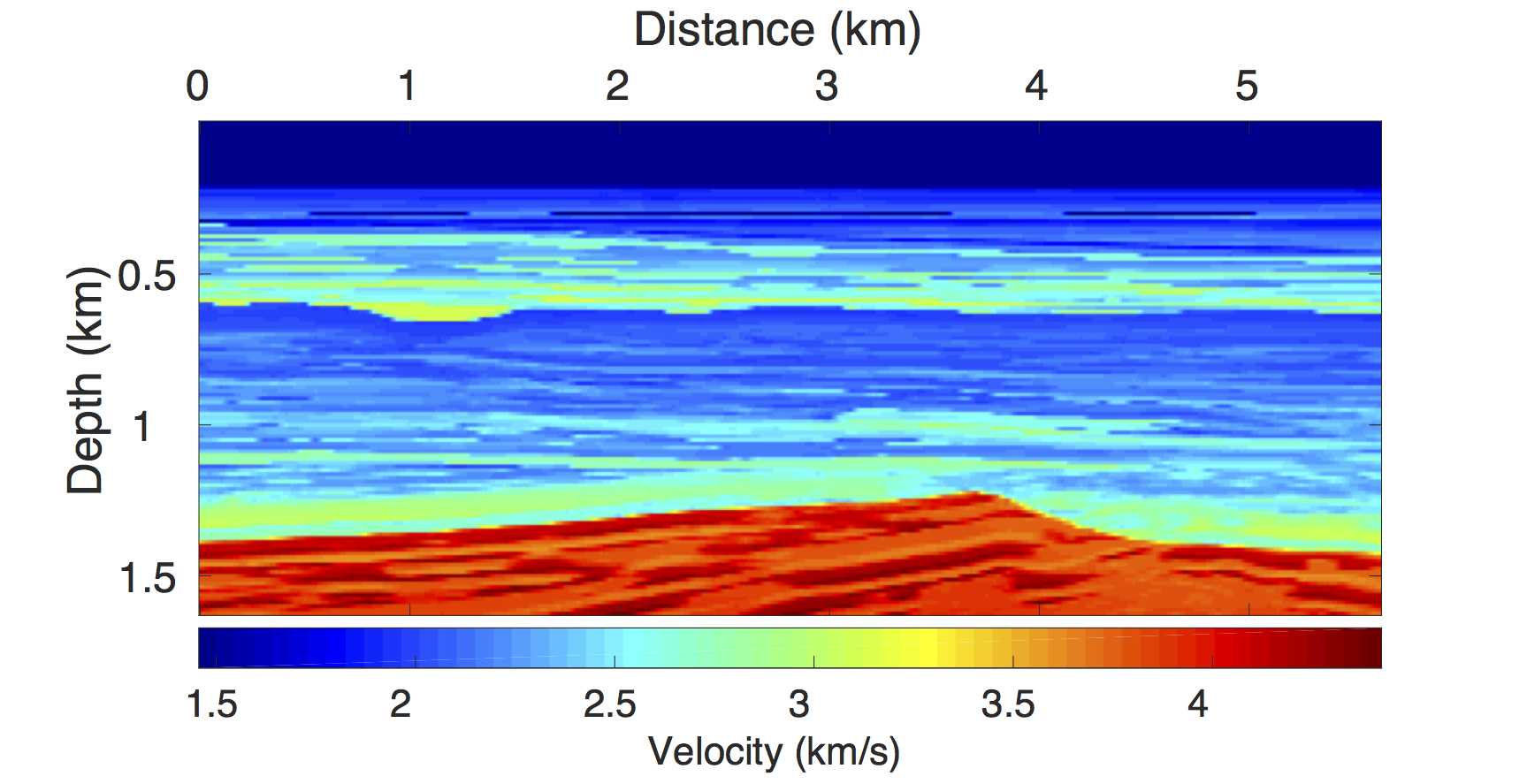
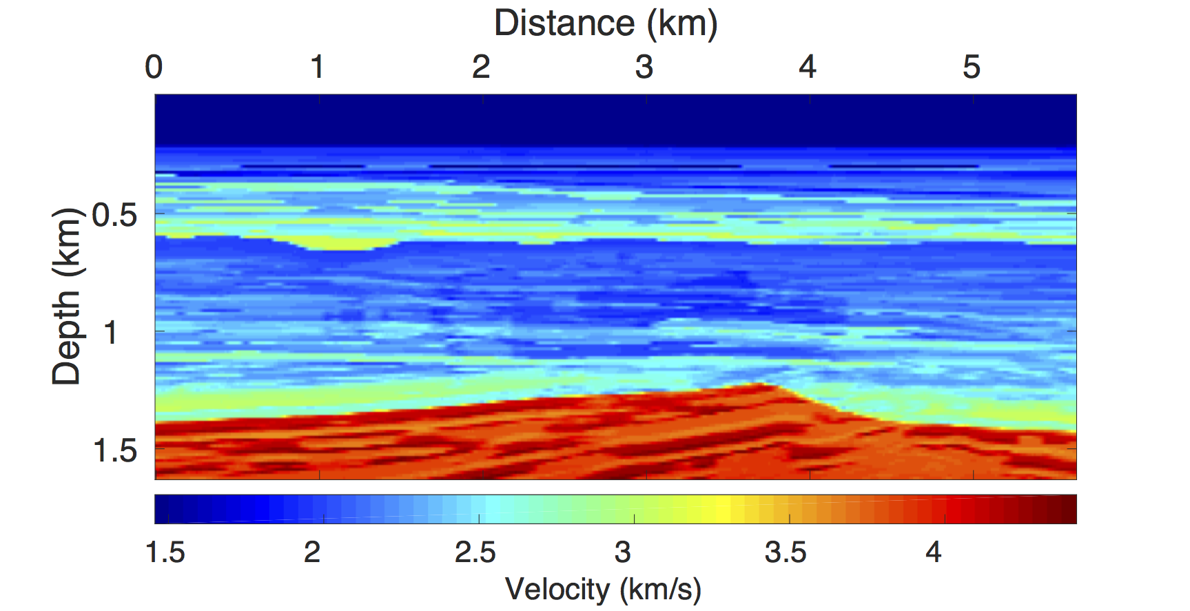
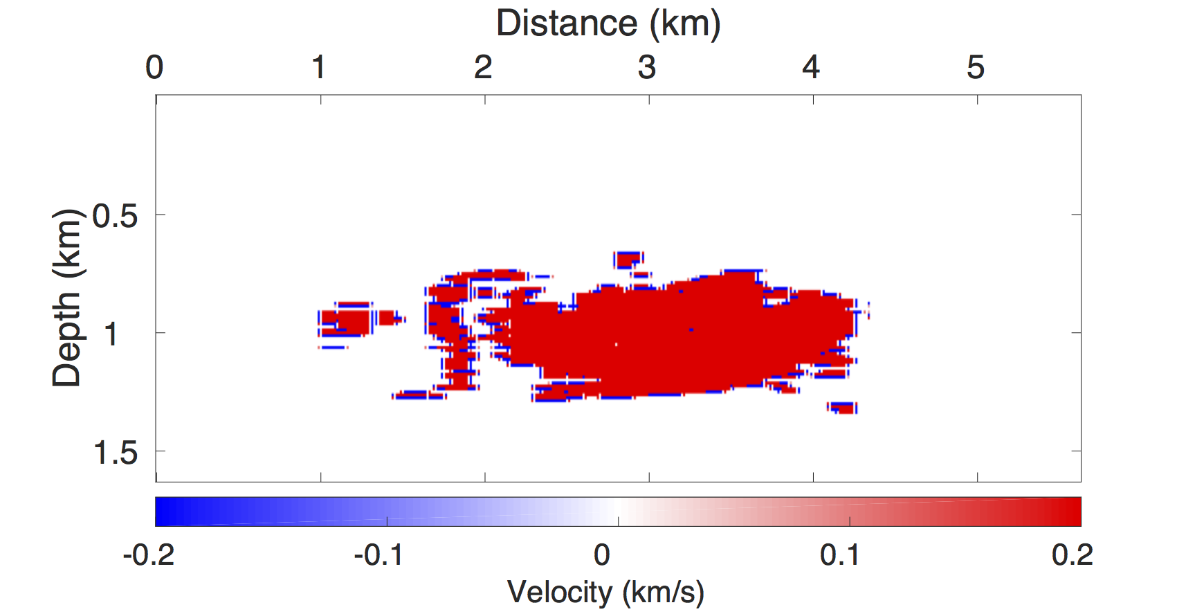
The SEAM model is a 3D deepwater subsalt earth model that includes a complex salt intrusive in a folded Tertiary basin. We select a 2D slice from the 3D model to generate a seismic line. Figure 13a shows a subset of the 2D slice used as the baseline model. We define the monitor model, Figure 13b, from the baseline model via fluid substitution resulting in a time-lapse difference under the overburden as shown in Figure 13c.
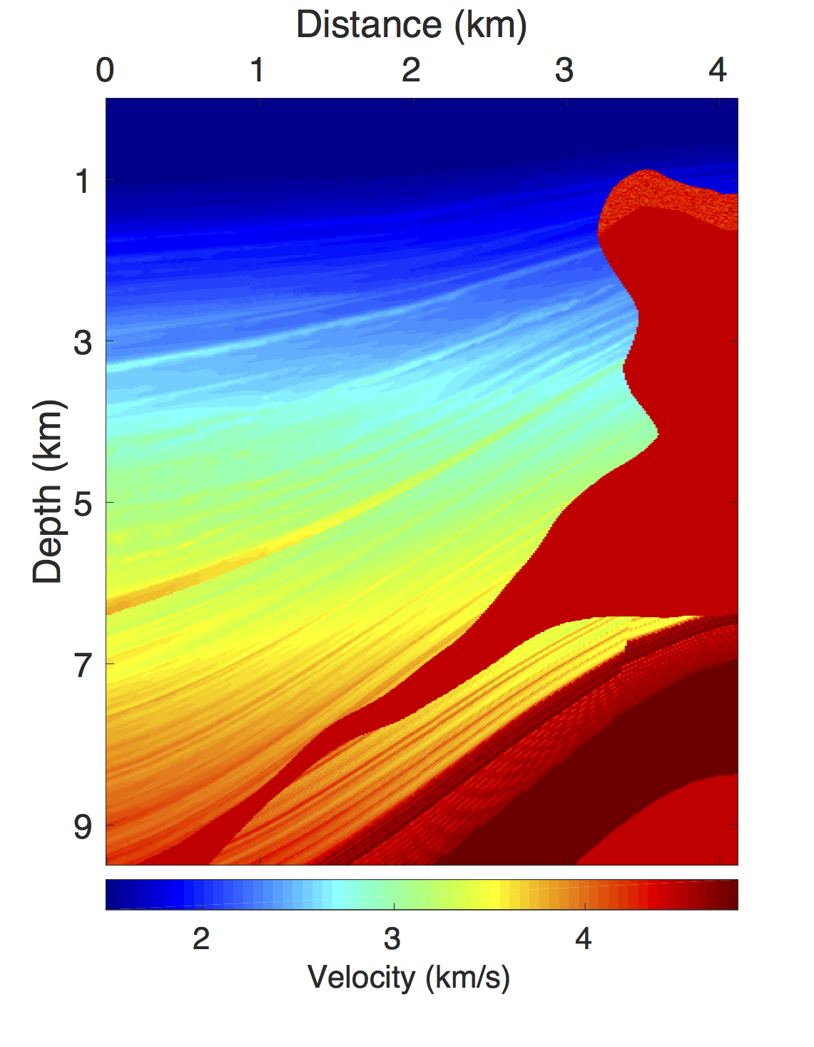

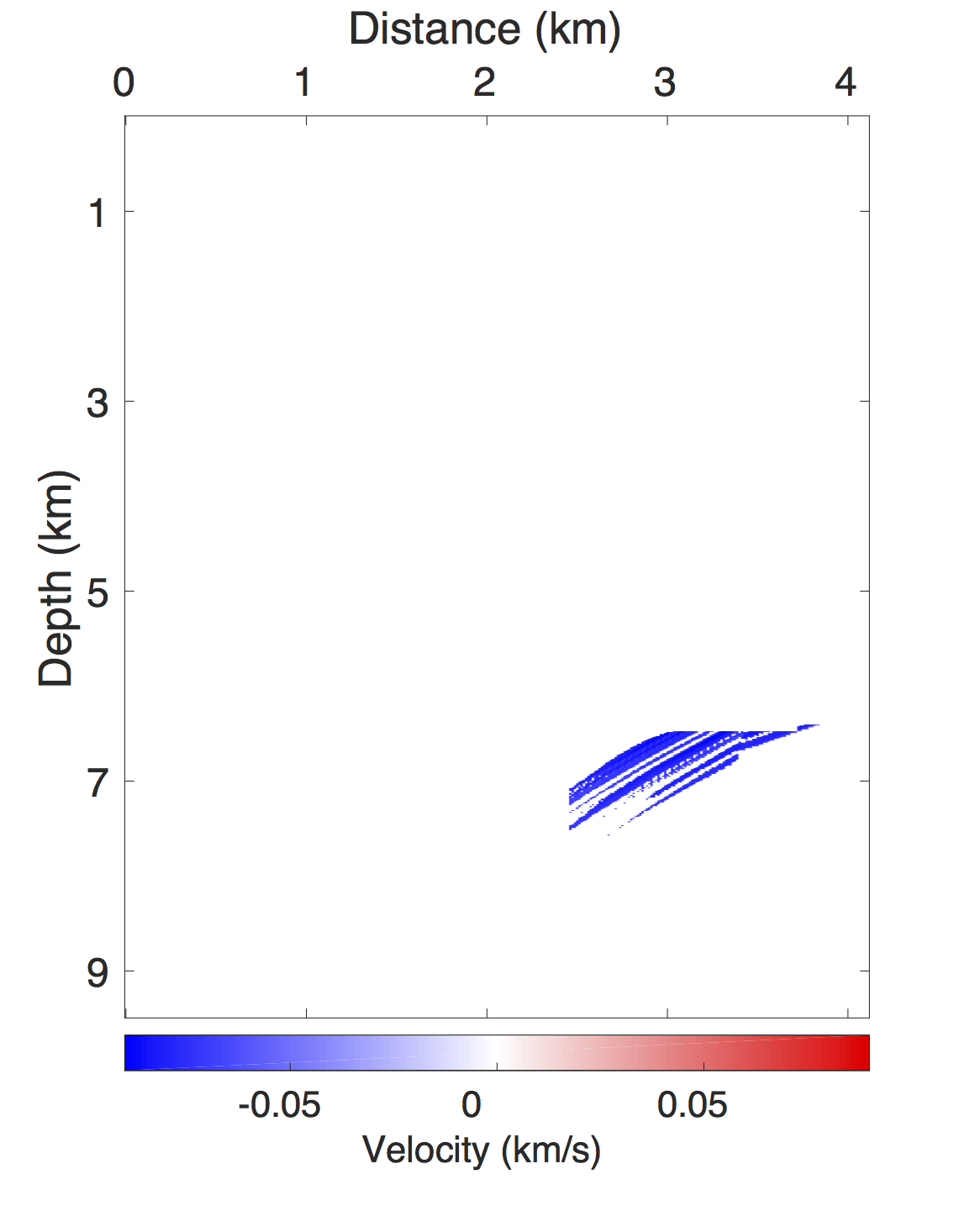
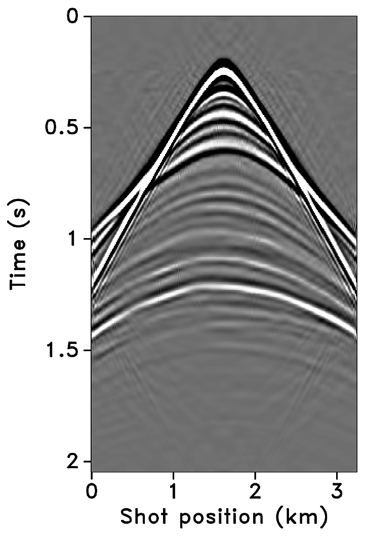
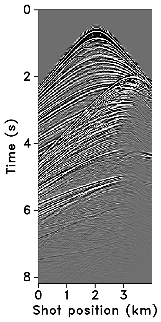
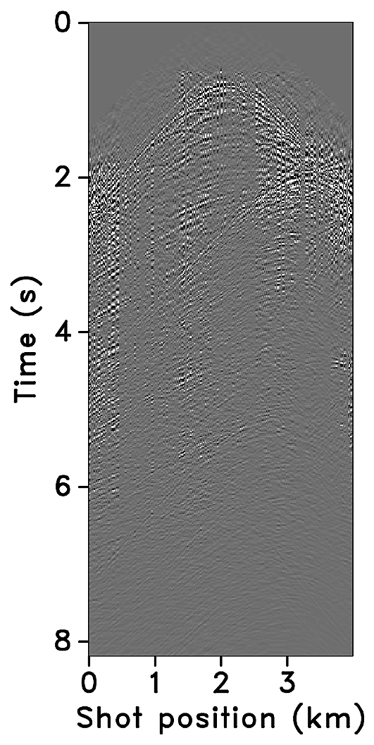
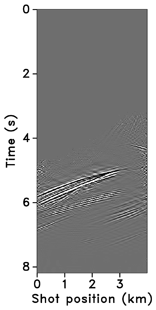
Using IWAVE (Symes, 2010), two acoustic data sets with a conventional source (and receiver) sampling of \(12.5\, \mathrm{m}\) are generated, one from the baseline model and the other from the monitor model. Each data set has \(N_t = 2048\) time samples, \(N_r = 320\) receivers and \(N_s = 320\) sources. The time sampling interval is \(0.004\, \mathrm{s}\). Subtracting the two data sets yields the time-lapse difference. Since no noise is added to the data, the time-lapse difference is simply the time-lapse signal. A receiver gather from the simulated baseline data, the monitor data and the corresponding time-lapse difference is shown in Figures 14a, 14b and 14c, respectively. Note that the amplitude of the time-lapse difference is one-tenth the amplitude of the baseline and monitor data. Therefore, in order to make the time-lapse difference visible, the color axis for the figures showing the time-lapse difference is one-tenth the color axis for the figures showing the baseline and monitor data. This colormap applies for the remainder of the paper. Given the spatial sampling of \(12.5\,\mathrm{m}\), the subsampling factor \(\eta\) for the time-jittered acquisition is \(2\). The number of measurements for each experiment is fixed—i.e., \(n = N/{\eta} = N/2\), each for \(\vector{y}_1\) and \(\vector{y}_2\).


We simulate a realization of the time-jittered marine acquisition with \(100\%\) overlap between the baseline and monitor surveys. Since our main aim is to analyze the effects of nonreplication of the time-lapse surveys on time-lapse data—i.e., when \(\vector{A_1} \neq \vector{A_2}\)—we compare recovery from the above case with the acquisition scenario that has least possible (or unavoidable) overlap between the time-lapse surveys only. Given the bigger size of the data set and limited computational resources, we restrict ourselves to one experiment for each case and a subsampling of \(\eta = 2\). Periodic densely sampled baseline and monitor data is recovered from the simultaneous data \(\vector{y}_1\) and \(\vector{y}_2\), respectively, by solving Equation \(\ref{eqjrm2}\). The inherent time-lapse difference is computed by subtracting the recovered baseline and monitor data.
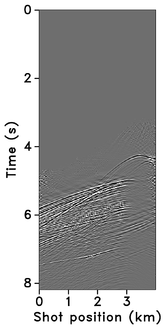
The recovered time-lapse data is colocated, regularized and interpolated to a fine uniform grid. We note that all the observations made for the BG COMPASS model, which is a relatively simpler model, hold true for the more complex SEAM model. Minimum overlap (or nonreplication) between time-lapse surveys improves recovery of the vintages since independent surveys give additional structural information. Hence, they serve as better input to extract certain poststack attributes used to study time-lapse differences. Figures 15a, 15b, 15c and 15d show the corresponding monitor data recovery. The SNR for the vintage recovery for minimum overlap between the surveys is \(30.2\,\mathrm{dB}\)—a significant improvement from the \(19.5\,\mathrm{dB}\) recovery for \(100\%\) overlap between the surveys. Moreover, as seen in Figures 15e, 15f, 15g and 15h, there is little variability in the recovery of the time-lapse difference from (the ideal) \(100\%\) overlap between the surveys to the more realistic almost nonreplicated surveys. The corresponding SNRs for the recovered time-lapse difference are \(9.6\,\mathrm{dB}\) for \(100\%\) overlap and \(4.1\,\mathrm{dB}\) for minimum overlap between the surveys. We note that the SNR for the minimum overlap between the surveys is biased due the presence of incoherent noise—between \(3.5\,\mathrm{s}\) to \(5.0\,\mathrm{s}\)—above the main time-lapse difference. If we compute the SNRs for the lower-half of the data that contains the time-lapse difference—i.e., after \(4.5\,\mathrm{s}\)—the SNR for minimum overlap between the surveys increases to \(6.8\,\mathrm{dB}\). More importantly, if we look at the plots themselves, we see that there is not much difference in the two recoveries. We are able to recover the primary arrivals and some reverberations below. Recall that the amplitude of the time-lapse difference is one-tenth the amplitude of the vintages. It is quite remarkable that we get good results given the complexity of the model and the low amplitude of the time-lapse difference. Recovery of the vintages and the time-lapse difference for a subsampling of \(\eta = 4\) follows the same trend as above.


Discussion
Realistic field seismic acquisitions suffer, amongst other possibly detrimental external factors, from irregular spatial sampling of sources and receivers. This poses technical challenges for the time-lapse seismic technology that currently aims to replicate densely sampled surveys for monitoring changes due to production. The experiments and synthetic results shown in the previous sections demonstrate favourable effects of irregular sampling and nonreplication of surveys on time-lapse data—i.e., decrease in replicability of the surveys leads to improved recovery of the vintages with little variability in the recovery of the time-lapse difference itself—while unraveling overlapping shot records. Note that we do not insist on replicating the irregular spatial positions in the field, however, the above observations hold as long as we know the irregular sampling positions after acquisition to a sufficient degree of accuracy, which is attainable in practice (see e.g., C. Mosher et al., 2014). Furthermore, we assume that there are no significant variations in the water column velocities, wave heights or temperature and salinity profiles amongst the different surveys while the source signature is also assumed to be the same. As long as these physical changes can be modeled, we do not foresee major problems. For instance, we expect that our approach can relatively easily be combined with source equalization (see e.g., Rickett and Lumley, 2001) and curvelet-domain matched filtering techniques (Beyreuther et al., 2005; Tegtmeier-Last and Hennenfent, 2013).
The proposed methodology involves a combination of economical randomized samplings with low environmental imprint and sparsity-promoting data recovery that aims to reduce cost of surveys and improve quality of the prestack time-lapse data without relying on expensive dense sampling and high degrees of replicability of the surveys. The combined operation of source separation, regularization and interpolation renders periodic densely sampled time-lapse data from time-compressed, and therefore economical, simultaneous, subsampled and irregular data. While the simultaneous data are separated reasonably well, recovery of the weak late-arriving events can be further improved by rerunning the recovery algorithm using the residual as input, using weighted one-norm minimization that exploits correlations between locations of significant transform-domain coefficients of different partitions—e.g., shot records, common-offset gathers, or frequency slices—of the acquired data (Mansour et al., 2013), etc. This needs to be examined in detail. Effects of noise and other physical changes in the environment also need to be carefully investigated. Nevertheless, as expected using standard CS, our recovery method should be stable with respect to noise (Candès et al., 2006b). Moreover, recent successes in the application of compressed sensing to land and marine field data acquisition (see e.g., C. Mosher et al., 2014) support the fact that technical challenges with noise and calibration can be overcome in practice.
Conclusions
We present an extension of our simultaneous time-jittered marine acquisition to time-lapse surveys for realistic, off-the-grid acquisitions where the sample points are known but do not coincide with a regular periodic grid. We conduct a series of synthetic seismic experiments with different random realizations of the simultaneous time-jittered marine acquisition to assess the effects of irregular sampling in the field on time-lapse data and demonstrate that dense, high-quality data recoveries are the norm and not the exception. We achieve this by adapting our proposed joint recovery method—a new and economic approach to randomized simultaneous time-lapse data acquisition that exploits transform-domain sparsity and shared information among different time-lapse recordings—to incorporate a regularization operator that maps traces from an irregular grid to a regular periodic grid. The recovery method is a combined operation of source separation, regularization and interpolation, wherein periodic densely sampled and colocated prestack data is recovered from time-compressed, and therefore economical, simultaneous, subsampled and irregular data.
We observe that with decrease in replication between the surveys—i.e., shot points are not replicated amongst the vintages—recovery of time-lapse data improve significantly with little variability in recovery of the time-lapse difference itself. We make this observation assuming source equalization and no significant changes in wave heights, water column velocities or temperature and salinity profiles, etc., amongst the different surveys. We also demonstrate the delicate reliance on exact replicability (between surveys) by showing that known deviations as small as average \(\pm (1, 2, 3)\, \mathrm{m}\) in shot positions of the monitor surveys from the baseline surveys vary recovery quality of the time-lapse difference—expressed as slight decrease or increase in the signal-to-noise ratios—and hence negate the efforts to replicate. Therefore, it would be better to focus on knowing what the shot positions were (post acquisition) than aiming to replicate. Moreover, since irregular spatial sampling is inevitable in the real world, the requirement for replicability in time-lapse surveys can perhaps be relaxed by embracing or better purposefully randomizing the acquisitions to maximize collection of information by effectively doubling the number of measurements for the common component, leading to surveys acquired at low cost and environmental imprint.
Acknowledgements
This work was financially supported in part by the Natural Sciences and Engineering Research Council of Canada Collaborative Research and Development Grant DNOISE II (CDRP J 375142-08). This research was carried out as part of the SINBAD II project with the support of the member organizations of the SINBAD Consortium. The authors wish to acknowledge the SENAI CIMATEC Supercomputing Center for Industrial Innovation, with support from BG Brasil and the Brazilian Authority for Oil, Gas and Biofuels (ANP), for the provision and operation of computational facilities and the commitment to invest in Research and Development. The authors would also like to thank the developers of the nonequispaced discrete Fourier transform (NFFT) toolbox (https://www-user.tu-chemnitz.de/~potts/nfft/).
Abma, R., Ford, A., Rose-Innes, N., Mannaerts-Drew, H., and Kommedal, J., 2013, Continued development of simultaneous source acquisition for ocean bottom surveys: In 75th eAGE conference and exhibition. doi:10.3997/2214-4609.20130081
Baron, D., Duarte, M. F., Wakin, M. B., Sarvotham, S., and Baraniuk, R. G., 2009, Distributed compressive sensing: CoRR, abs/0901.3403. Retrieved from http://arxiv.org/abs/0901.3403
Beasley, C. J., 2008, A new look at marine simultaneous sources: The Leading Edge, 27, 914–917. doi:10.1190/1.2954033
Berkhout, A. J., 2008, Changing the mindset in seismic data acquisition: The Leading Edge, 27, 924–938. doi:10.1190/1.2954035
Beyreuther, M., Cristall, J., and Herrmann, F. J., 2005, Computation of time-lapse differences with 3-D directional frames: SEG technical program expanded abstracts. doi:10.1190/1.2148227
Candès, E. J., Demanet, L., Donoho, D., and Ying, L., 2006a, Fast discrete curvelet transforms: Multiscale Modeling & Simulation, 5, 861–899. doi:DOI:10.1137/05064182X
Candès, E. J., Romberg, J., and Tao, T., 2006b, Stable signal recovery from incomplete and inaccurate measurements: Communications on Pure and Applied Mathematics, 59, 1207–1223. doi:10.1002/cpa.20124
Donoho, D. L., 2006, Compressed sensing: Information Theory, IEEE Transactions on, 52, 1289–1306.
Hampson, G., Stefani, J., and Herkenhoff, F., 2008, Acquisition using simultaneous sources: The Leading Edge, 27, 918–923. doi:10.1190/1.2954034
Hennenfent, G., and Herrmann, F. J., 2006, Seismic denoising with non-uniformly sampled curvelets: Computing in Science and Engineering, 8, 16–25.
Hennenfent, G., and Herrmann, F. J., 2008, Simply denoise: Wavefield reconstruction via jittered undersampling: Geophysics, 73, V19–V28.
Hennenfent, G., Fenelon, L., and Herrmann, F. J., 2010, Nonequispaced curvelet transform for seismic data reconstruction: A sparsity-promoting approach: Geophysics, 75, WB203–WB210. Retrieved from https://www.slim.eos.ubc.ca/Publications/Public/Journals/Geophysics/2010/hennenfent2010GEOPnct/hennenfent2010GEOPnct.pdf
Kok, R. de, and Gillespie, D., 2002, A universal simultaneous shooting technique: In 64th eAGE conference and exhibition.
Kumar, R., Wason, H., and Herrmann, F. J., 2015, Source separation for simultaneous towed-streamer marine acquisition — a compressed sensing approach: Geophysics, 80, WD73–WD88. doi:10.1190/geo2015-0108.1
Kunis, S., 2006, Nonequispaced FFT: Generalisation and inversion: PhD thesis,. Lübeck University.
Landrø, M., 2001, Discrimination between pressure and fluid saturation changes from time-lapse seismic data: Geophysics, 66, 836–844.
Li, C., Mosher, C. C., and Kaplan, S. T., 2012, Interpolated compressive sensing for seismic data reconstruction: SEG technical program expanded abstracts. doi:10.1190/segam2012-1335.1
Lumley, D., and Behrens, R., 1998, Practical issues of 4D seismic reservoir monitoring: What an engineer needs to know: SPE Reservoir Evaluation & Engineering, 1, 528–538.
Mallat, S., 2008, A wavelet tour of signal processing: The sparse way: Academic press.
Mansour, H., Herrmann, F. J., and Yilmaz, O., 2013, Improved wavefield reconstruction from randomized sampling via weighted one-norm minimization: Geophysics, 78, V193–V206. doi:10.1190/geo2012-0383.1
Mansour, H., Wason, H., Lin, T. T., and Herrmann, F. J., 2012, Randomized marine acquisition with compressive sampling matrices: Geophysical Prospecting, 60, 648–662.
Moldoveanu, N., and Quigley, J., 2011, Random sampling for seismic acquisition: In 73rd eAGE conference & exhibition.
Mosher, C., Li, C., Morley, L., Ji, Y., Janiszewski, F., Olson, R., and Brewer, J., 2014, Increasing the efficiency of seismic data acquisition via compressive sensing: The Leading Edge, 33, 386–391.
Potts, D., Steidl, G., and Tasche, M., 2001, Modern Sampling Theory: Mathematics and Applications:, 249–274.
Rickett, J., and Lumley, D., 2001, Cross-equalization data processing for time-lapse seismic reservoir monitoring: A case study from the gulf of mexico: Geophysics, 66, 1015–1025.
Spetzler, J., and Kvam, Ø., 2006, Discrimination between phase and amplitude attributes in time-lapse seismic streamer data: Geophysics, 71, O9–O19.
Symes, W. W., 2010, IWAVE: A framework for wave simulation:. Retrieved from http://www.trip.caam.rice.edu/software/iwave/doc/html/
Tegtmeier-Last, S., and Hennenfent, G., 2013, System and method for processing 4D seismic data:. Google Patents. Retrieved from http://www.google.com/patents/US20130253838
Wason, H., and Herrmann, F. J., 2013, Time-jittered ocean bottom seismic acquisition: SEG technical program expanded abstracts. doi:10.1190/segam2013-1391.1
Xu, S., Zhang, Y., Pham, D., and Lambare, G., 2005, Antileakage Fourier transform for seismic data regularization: Geophysics, 70, V87–V95.